Article

A Practical Split-Window Algorithm for Retrieving Land Surface Temperature from Landsat-8 Data and a Case Study of an Urban Area in China

1
College of Architecture and Civil Engineering, Taiyuan University of Technology, Yingze Street 79, Taiyuan 030024, China
2
Institute of Geodesy and Geophysics, Chinese Academy of Sciences, Xudong Street 340, Wuhan 430077, China
3
Shanxi Administration of Surveying, Mapping and Geoinformation, Yingze Street 136, Taiyuan 030001, China
4
Wanfang College of Science & Technology, Henan Polytechnic University, Qiancheng North Road 8, Vocational Education Park, Zhengzhou 451400, China
*
Author to whom correspondence should be addressed.
Remote Sens. 2015, 7(4), 4371-4390; https://doi.org/10.3390/rs70404371
Submission received: 4 January 2015 / Revised: 26 February 2015 / Accepted: 30 March 2015 / Published: 14 April 2015
(This article belongs to the Special Issue Recent Advances in Thermal Infrared Remote Sensing)

Abstract

:
This paper proposes a practical split-window algorithm (SWA) for retrieving land surface temperature (LST) from Landsat-8 Thermal Infrared Sensor (TIRS) data. This SWA has a universal applicability and a set of parameters that can be applied when retrieving LSTs year-round. The atmospheric transmittance and the land surface emissivity (LSE), the essential SWA input parameters, of the Landsat-8 TIRS data are determined in this paper. We also analysed the error sensitivity of these SWA input parameters. The accuracy evaluation of the proposed SWA in this paper was conducted using the software MODTRAN 4.0. The root mean square error (RMSE) of the simulated LST using the mid-latitude summer atmospheric profile is 0.51 K, improving on the result of 0.93 K from Rozenstein (2014). Among the 90 simulated data points, the maximum absolute error is 0.99 °C, and the minimum absolute error is 0.02 °C. Under the Tropical model and 1976 US standard atmospheric conditions, the RMSE of the LST errors are 0.70 K and 0.63 K, respectively. The accuracy results indicate that the SWA provides an LST retrieval method that features not only high accuracy but also a certain universality. Additionally, the SWA was applied to retrieve the LST of an urban area using two Landsat-8 images. The SWA presented in this paper should promote the application of Landsat-8 data in the study of environmental evolution.

Graphical Abstract

1. Introduction

Land surface temperature (LST) plays a significant role in environmental evolution, including heat energy circulation and the water cycle. Retrieving LST from remote sensing data is an important capability for researching the spatial evolution of the regulation of the heat environment at local and global scales [1,2,3,4]. Studies on the derivation of LST using satellites have been conducted primarily using NOAA AVHRR data [5,6] at a regional scale. Landsat Thematic Mapper (TM) and Enhanced Thematic Mapper Plus (ETM+) thermal infrared (TIR) data have been used in local-scale studies of LST distributions [7,8,9]. Data from medium-resolution thermal infrared sensors, such as MODIS and AVHRR with daily temporal resolution, and high-resolution thermal infrared sensors, such as the Landsat series that pass once every 16 days, have been supplied to the public in recent decades [10]. Many studies on the retrieval of LSTs from satellite TIR data have been performed since the 1990s. The methods used can be broadly classified into three categories: single-channel methods, multi-channel methods, and multi-angle methods [11]. The single-channel method, also called the mono-window algorithm, utilizes the radiance measured by a sensor in a single channel to retrieve LST using the general radiance transfer equation [12,13,14]. The multi-channel method, also called the split-window algorithm (SWA), uses the different absorptions of two TIR channels, linearizing or nonlinearizing the radiance transfer equation with respect to the temperature or wavelength. Many efforts have been made to extend the SWA because these algorithms assume that the land surface emissivity (LSE) values in both TIR channels are known [15,16,17,18,19,20,21,22,23,24,25,26,27]. The multi-angle method is in accordance with different atmospheric absorptions because of the differential path-lengths associated with observing the same object from various viewing angles [21,24,28,29,30,31,32]. The launch of the Landsat-8 satellite on February 11, 2013 adds to the remote sensing data of the Landsat family, TM and ETM+. The Landsat-8 satellite carries the Operational Land Imager (OLI) with nine bands and Thermal Infrared Sensor (TIRS) with band10 and band11. Using an SWA, the TIRS band10 and band11 provide the atmospheric rectification for the thermal infrared data [33,34]. Jimenez-Munoz and Sobrino et al. [35], Rozenstein et al. [10] and Du et al. [36] proposed three different SWAs for LST retrieval from Landsat-8 TIR data. The objective of this paper is to provide another SWA for retrieving LSTs from Landsat-8 data. We attempt to improve the convenience and accuracy of the LST retrieval of Landsat-8 TIR data and provide an alternative. Although the idea of the SWA presented in this paper is based on the practical split-window algorithm proposed by Mao et al. [27], we did not merely transplant Mao’s principle; we also studied the input parameter determination and algorithm structures. We conclude that the SWA idea proposed in this study can be not only applied to Landsat-8 TIR data but can also be used with other kinds of remotely sensed thermal infrared data, such as ASTER and MODIS.
In this paper, we have developed a practical SWA for Landsat-8 TIRS data from another perspective and subjected it to a sensitivity analysis and accuracy assessment. Additionally, a specific calculated case for an urban area in China is provided. Specifically, this paper will (1) describe the SWA model and derive the LST calculation; (2) determine the atmospheric transmittance and the emissivity of the ground for the Landsat-8 TIRS; (3) analyse the sensitivity of the essential input parameters and assess the accuracy via simulated data using MODTRAN 4.0; and (4) retrieve the LST of an urban area in China.

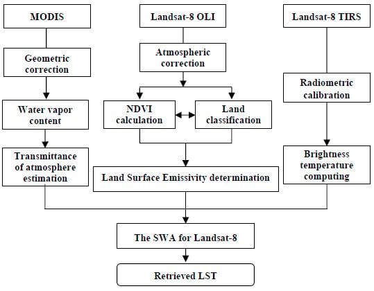
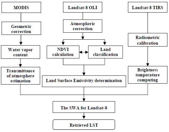
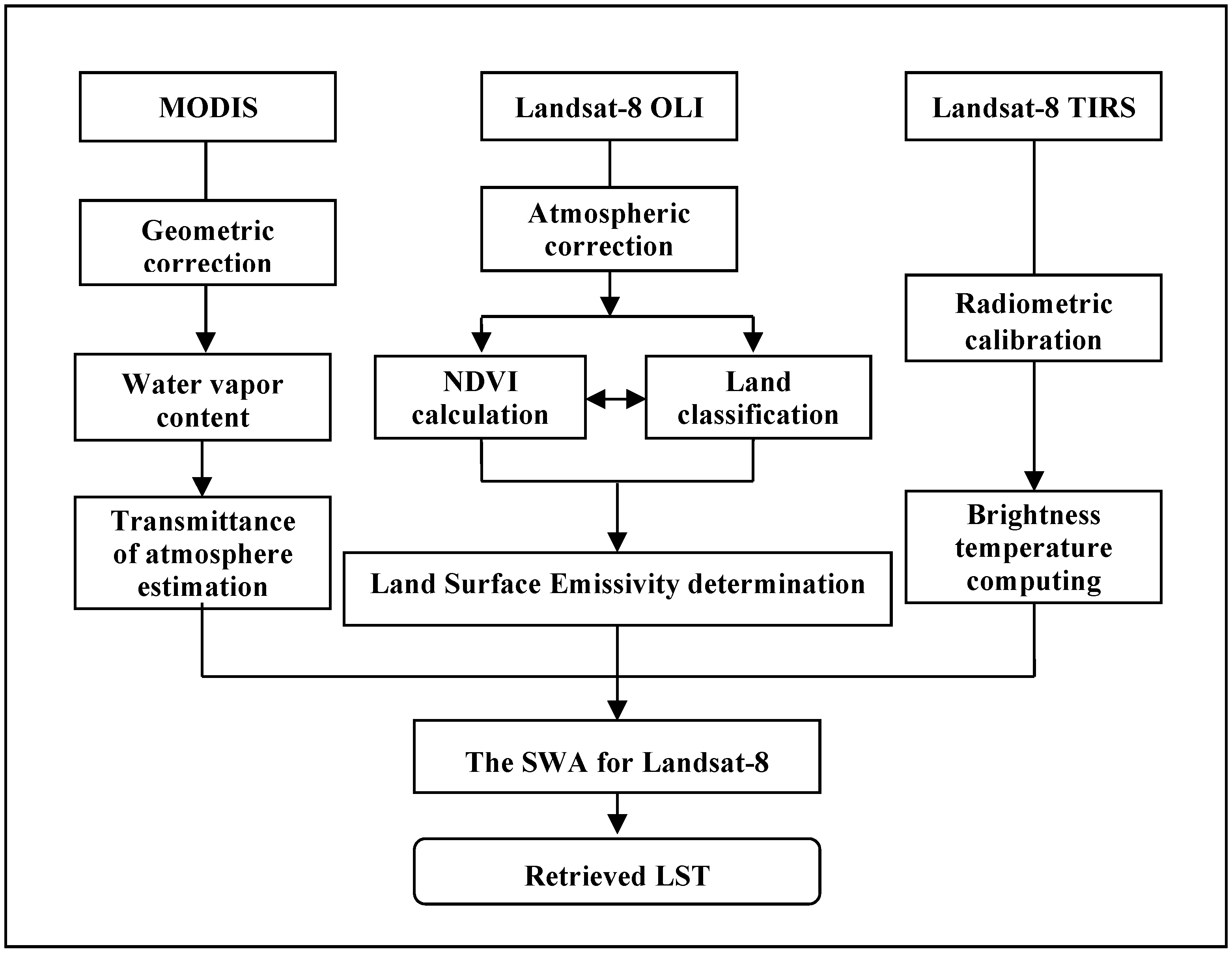
2. The SWA for Landsat-8 TIRS

2.1. Theoretical Derivation of the SWA

The theoretical basis of the LST retrieval algorithm is Planck’s law, which is based on the thermal radiance of the ground and the heat transfer from the ground through the atmosphere to the remote sensor [27]. According to Planck’s law, the thermal emittance from an object can be expressed as Planck’s radiance function [37], as follows in Equation (1):
B n ( T ) = 2 h c 2 n 3 e h c n k T 1
where Bn(T) denotes the object’s spectral radiance, T its absolute temperature, k the Boltzmann constant, h the Planck constant, and c the speed of light. The units of Bn(T) are Wm−2sr−1µm−1. The general radiance transfer equation [38] for the remote sensing of LST can be formulated as follows in Equation (2):
B i ( T i ) = ε i τ i B i ( T s ) + τ i ( 1 ε i ) I i + I i
where Ts is the LST, Ti is the brightness temperature in channel i, εi is the ground emissivity and τi is the atmospheric transmittance in band i. Bi(Ts) is the ground radiance, and Ii ↓ and Ii ↑ are the downward and upward path radiances, respectively. Ii ↓ and Ii ↑ can be expressed by Equations (3) and (4), respectively [27]:
I i = ( 1 τ i ) B i ( T a )
where T a is the average temperature of the downward radiance of the atmosphere, and Ta is the average temperature of the upward radiance of atmosphere. Every term of the radiance transfer equation includes the Planck function. According to Qin’s [39] analysis, few differences result from using Ta instead of T a . Therefore, Equation (2) can be written as follows:
B i ( T i ) = ε i τ i B i ( T s ) + τ i ( 1 ε i ) ( 1 τ i ) B i ( T a ) + ( 1 τ i ) B i ( T a )
which can be consolidated as follows:
B i ( T i ) = ε i τ i B i ( T s ) + ( 1 τ i ) ( 1 + ( 1 ε i ) τ i ) B i ( T a )
In Equation (6), the value of Bi(Ti) can be calculated by substituting the brightness temperature T i into the Planck function. The terms Bi(Ts) and Bi(Ta) need to be simplified. In this paper, considering the scope of the application and the desired retrieval accuracy, we applied different simplified fitting methods for Bi(Ts) and Bi(Ta). Because Bi(Ts) has a greater impact on the retrieval precision and it contains inversion parameters, we decided to nonlinearly fit it with a quadratic function, whereas Bi(Ta), which has less impact on the retrieval accuracy, can be linearly fit. Then, Equation (6) can be written as follows:
ε i τ i ( a i T s 2 + b i T s + c i ) + ( 1 τ i ) ( 1 + ( 1 ε i ) τ i ) ( k i T a + d i ) B i ( T i ) = 0
If the equation is condensed by setting
{ A i = ε i τ i a i B i = ε i τ i b i C i = ( 1 τ i ) ( 1 + ( 1 ε i ) τ i ) k i D i = ε i τ i c i + ( 1 τ i ) ( 1 + ( 1 ε i ) τ i ) d i B i ( T i ) B i ( T i ) = 2 h c 2 n 3 / ( e h c n i k T i 1 )
Then, Equation (7) can be expressed as follows:
A i T s 2 + B i T s + C i T a + D i = 0
For Landsat-8 TIRS band10 and band11, Equation (8) generates the following equation set:
{ A 10 T s 2 + B 10 T s + C 10 T a + D 10 = 0 A 11 T s 2 + B 11 T s + C 11 T a + D 11 = 0
or, upon consolidation,
( C 11 A 10 C 10 A 11 ) T s 2 + ( C 11 B 10 C 10 B 11 ) T s + ( C 11 D 10 C 10 D 11 ) = 0
When this equation is solved for Ts, the result can be expressed as
T s = [ ( C 10 B 11 C 11 B 10 ) + ( C 10 B 11 C 11 B 10 ) 2 4 ( C 11 A 10 C 10 A 11 ) ( C 11 D 10 C 10 D 11 ) ] / [ 2 ( C 11 A 10 C 10 A 11 ) ]
which can be generalized to:
( T s + ξ ) 2 = [ α B 10 ( T 10 ) β B 11 ( T 11 ) ] + ψ
where ξ , α , β , and ψ are parameters computed by τ 10 , ε 10 , τ 11 , and ε 11 , respectively.

2.2. Determination of Coefficients

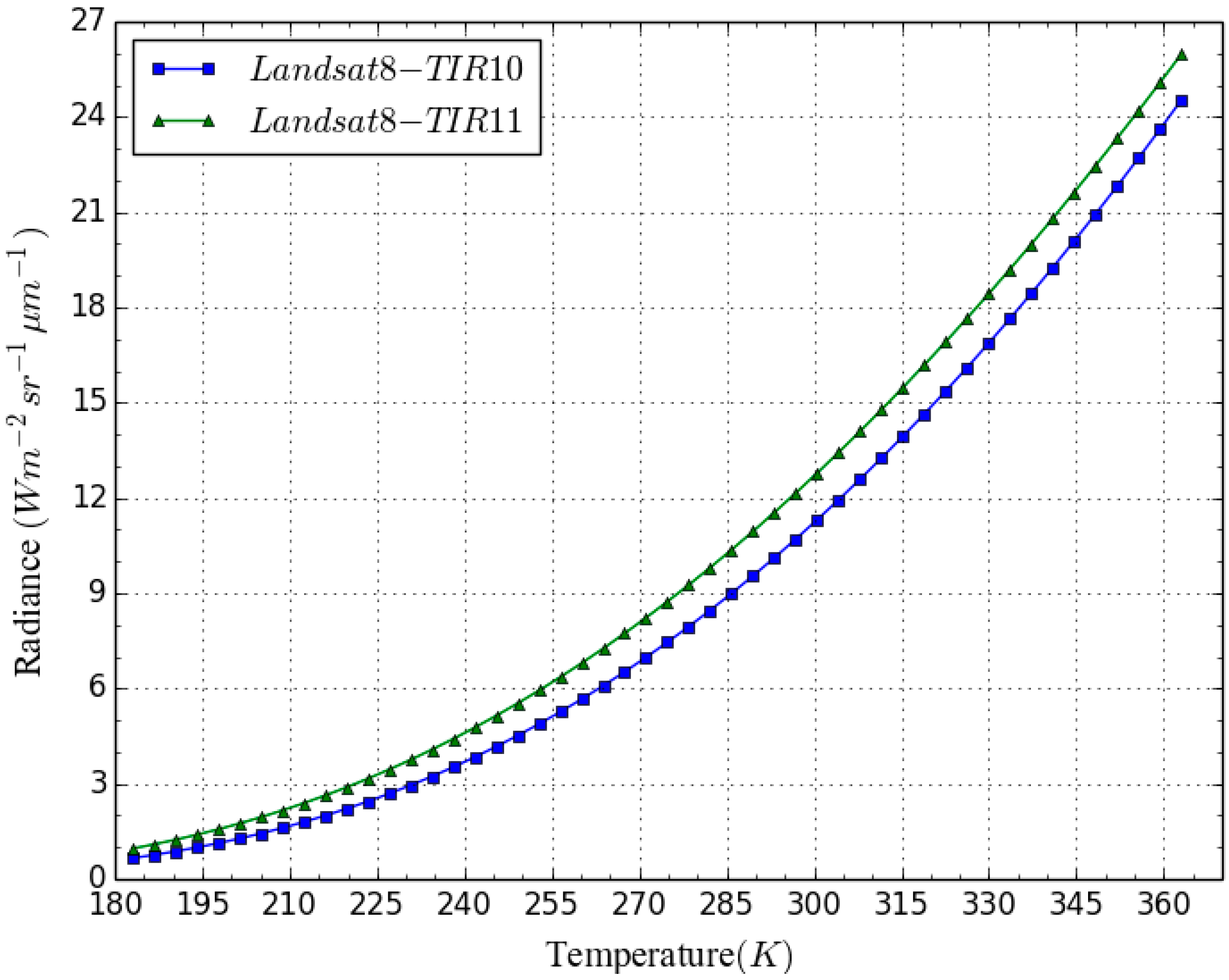
2.2.1. Determination of the Fitting Parameters for B i ( T s ) and B i ( T a )

This study simplified Bi(Ts) via a quadratic fitting method and Bi(Ta) via a linear simplification approach. To strengthen the universality of the model, the temperature range is set from 180 K–363 K (−90 °C–90 °C) for Landsat-8 thermal infrared bands 10 and 11. The selection of the temperature range is based on a full consideration of the existence of extreme surface temperature regions. The extreme minimum temperature was reported to have reached −71 °C in Oymyakon village in Russia, and the surface temperature reached as high as 82.3 °C in several desert areas in the summer. Based on the TIR spectral response function of Landsat-8, the effective wavelengths [40] and wavenumbers of these TIRS are calculated to be 10.9034 μm and 917.1417608 cm−1 for the minimum temperature, respectively, and 12.0028 μm and 833.1387464 cm−1 for the maximum temperature, respectively. Then, the thermal radiation values can be obtained using Equation (1). The corresponding Planck curve is shown in Figure 1. The quadratic fitting function is shown in Table 1, the linear regression formula is listed in Table 2, and the fitting parameters Bi(Ts) and Bi(Ta) are listed in Table 3.
Figure 1. The Planck radiance-temperature (180 K–363 K) curve of the Landsat-8 TIRS.
Remotesensing 07 04371 g001
Table 1. The quadratic fitting results for the Landsat-8 TIRS.
TIRSQuadratic Fitting ExpressionR2SEE
band10 B 10 ( T s ) = 0.0006678 T s 2 0.2333226 T s + 21.1666266 0.9999790.0309
band11 B 11 ( T s ) = 0.0006188 T s 2 0.1990475 T s + 16.7224278 0.9999970.0117
Table 2. The linear regression results for the Landsat-8 TIRS.
TIRSLinear Regression ResultsR2SEE
band10 B 10 ( T a ) = 0.1312942 T a 26.7808503 0.94651.6404
band11 B 11 ( T a ) = 0.1387986 T a 27.7043284 0.95841.5193
Table 3. The fitting parameters of Bi(Ts) and Bi(Ta) for the Landsat-8 TIRS.
TIRSFitting Parameters
Quadratic Fitting ParametersLinear Regression Parameters
B i ( T s ) = a i T s 2 + b i T s + c i B i ( T a ) = k i T a + d i
band10a10 = 0.0006678 b10 = −0.2333226 c10 = 21.1666266k10 = 0.1312942 d10 = −26.7808503
band11a11 = 0.0006188 b11 = −0.1990475 c11 = 16.7224278k11 = 0.1387986 d11 = −27.7043284

2.2.2. Determination of Atmospheric Transmittance

The atmospheric transmittance is an important factor in the split-window algorithm. According to previous studies, the atmospheric transmittance strongly depends on the atmospheric water vapour content, especially for thermal bands [27]. This paper studied the relationship between the Landsat-8 TIRS’ atmospheric transmittance estimates and the water vapour in the atmosphere via MORTRAN 4.0 simulations that use the Mid-Latitude Summer atmosphere profile. The simulation data are listed in Table 4. Cubic polynomial fits are adopted for the relationship between the atmospheric water vapour content and transmittance, and the fitting expressions are shown in Table 5. The agreement is very satisfactory. Because the errors in the water vapour content are 0.20 g·cm−2 [41] and 0.10 g·cm−2, the corresponding atmospheric transmittance evaluation errors are less than 0.031 and 0.016, respectively.
Table 4. The water vapour of the atmosphere and the corresponding atmospheric transmittance as simulated by MORTRAN 4.0.
Water Vapour Content (g·cm−2)TIR10- τ 10 TIR11- τ 11
0.50.935420.89660
0.60.929030.88448
0.70.922170.87220
0.80.914830.85967
0.90.907000.84686
1.00.898690.83372
1.10.889900.82021
1.20.880640.80637
1.30.870930.79215
1.40.860760.77758
1.50.850150.76266
1.60.839130.74742
1.70.827690.73187
1.80.815880.71603
1.90.803700.69993
2.00.791170.68360
2.10.778300.66706
2.20.765140.65034
2.30.751680.63347
2.40.737980.61649
2.50.724010.59941
2.60.709830.58229
2.70.695460.56512
2.80.680920.54797
2.90.666220.53084
3.00.651400.51378
Table 5. The cubic fit regression functions of the atmospheric transmittance and water vapour content range of 0.5–3.0 g·cm−2.
TIRSCubic Regression ResultsR2SEE
band10 τ 10 = 0.9570356 0.0277340 w 0.0333734 w 2 + 0.0028800 w 3 0.9999990.0001
band11 τ 11 = 0.9456728 0.0857755 w 0.0290912 w 2 + 0.0032169 w 3 0.9999950.0003
The water vapour content w was estimated using the same daytime MODIS data. Although the times of MODIS and Landsat-8 cannot be strictly the same, the Terra satellite carrying MODIS transits the study area approximately 43 minutes earlier than Landsat-8 ((approximately 02:35 versus approximately 03:08). The study area is ringed by mountains on three sides, and we have therefore assumed that the water vapour content w is constant during this time. Kaufmann, Y. J. et al. [42] provided a method to compute the water vapour content in the atmosphere using the reflectance of band2 and band19 of MODIS; thus, we can obtain the water vapour content of the atmosphere using Equation (13).
w = ( α ln ( r 19 / r 2 ) β ) 2
where w is the water vapour content in g·cm−2, α = 0.020 , β = 0.651 , and r 19 and r 2 denote the reflectance of MODIS band19 and band2, respectively.

2.2.3. Determination of the Emissivity of the Ground

In consideration of the high signal-to-noise ratio (SNR), this study employed the NDVI threshold method, which considers the differing impacts of distinct land cover types (e.g., water, vegetation, bare soil and impervious surfaces), proposed by Sobrino et al. [43] to determine the land surface emissivity (LSE).
We have also referred to the ASTER spectral database [44] to determine the emissivity values of water, vegetation and non-vegetation for Landsat-8 TIRS band10 and band11 (Table 6). Water pixels with negative NDVI values (NDVI < 0) were set to LSE values of 0.991 and 0.986 for band10 and band11, respectively. Fully vegetated pixels with a NDVI value greater than 0.50 were set to LSE values of 0.984 and 0.980. Non-water pixels with NDVI less than 0.20 are considered to be non-vegetated areas, and the LSE values of these pixels were set to 0.964 and 0.970. Finally, pixels with NDVI values greater than 0.20 and less than 0.50 are considered to be mixed pixels incorporating various degrees of vegetation and non-vegetation. The LSE values of these pixels were calculated using Equations (14) and (15) [45,46,47].
ε i m i x = ε i v p v + ε i n ( 1 p v ) + ( 1 ε i n ) ( 1 p v ) F ε i v
p v = ( N D V I N D V I m i n N D V I max N D V I m i n ) 2
where εimix is the emissivity of the mixed pixels for band10 and band11, εiv is the emissivity of the fully vegetated pixels for band10 and band11, εin is the emissivity of the non-water and non-vegetated pixels for band10 and band11, and F = 0.55 is a shape factor considering the geometrical distribution [48]. The parameter pv is the scaled NDVI value, in which NDVImin and NDVImax are the NDVI values for non-vegetated and fully vegetated land covers, respectively. Please note that, in recent years, colourful steel plates mainly composed of electro-galvanized steels have been installed in architectural fields, with blue-coloured plates being especially common. As a result, regions with blue roof plates in our study area are relatively prevalent. Because the corresponding NDVI of these blue colour steels is relatively large, generally above 0.20 and sometimes even as high as 0.53, we separated these areas from the 0.20–0.50 range of NDVI to produce amplitude ratio values. According to the ASTER spectral database, the Roofing Materials--Galvanized Steel Metal category features wavelengths of 10.9009 μm and 12.0108 μm and corresponding reflectances of 0.041 and 0.038. Therefore, we calculated the Galvanized Steel Metal emissivity values in band10 and band11 to be 0.959 and 0.962, respectively.
Table 6. The emissivity values of water, vegetation and non-vegetation for Landsat-8 TIRS band10, and band11.
εwaterεvegetationεnon-vegetationεGalvanized-Steel
TIR-band100.9910.9840.9640.959
TIR-band110.9860.9800.9700.962

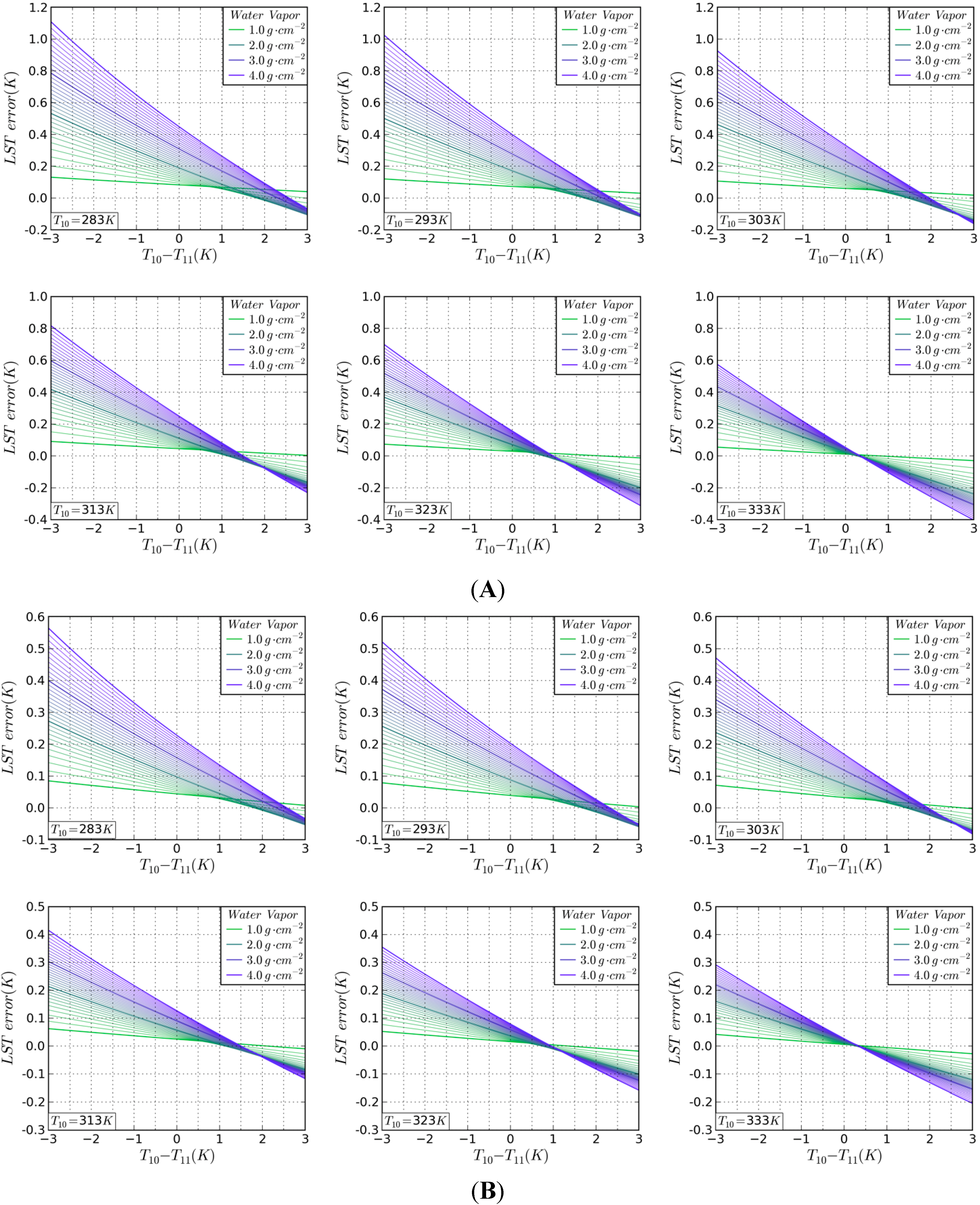
3. Steadiness Analysis and Validation of the SWA

3.1. Steadiness Analysis of the SWA

To assess the steadiness of the SWA proposed in the paper, we analysed the impact of misestimated SWA input parameters on the LST derivation error. The atmospheric transmittance calculated through the atmosphere’s water vapour content and the LSE play a major role in the SWA; thus, the influences of these two input parameters were analysed. To enable comparison with the existing SWA proposed by Rozenstein et al. (2014), the parameter values were kept almost consistent with that of Rozenstein et al. (2014).

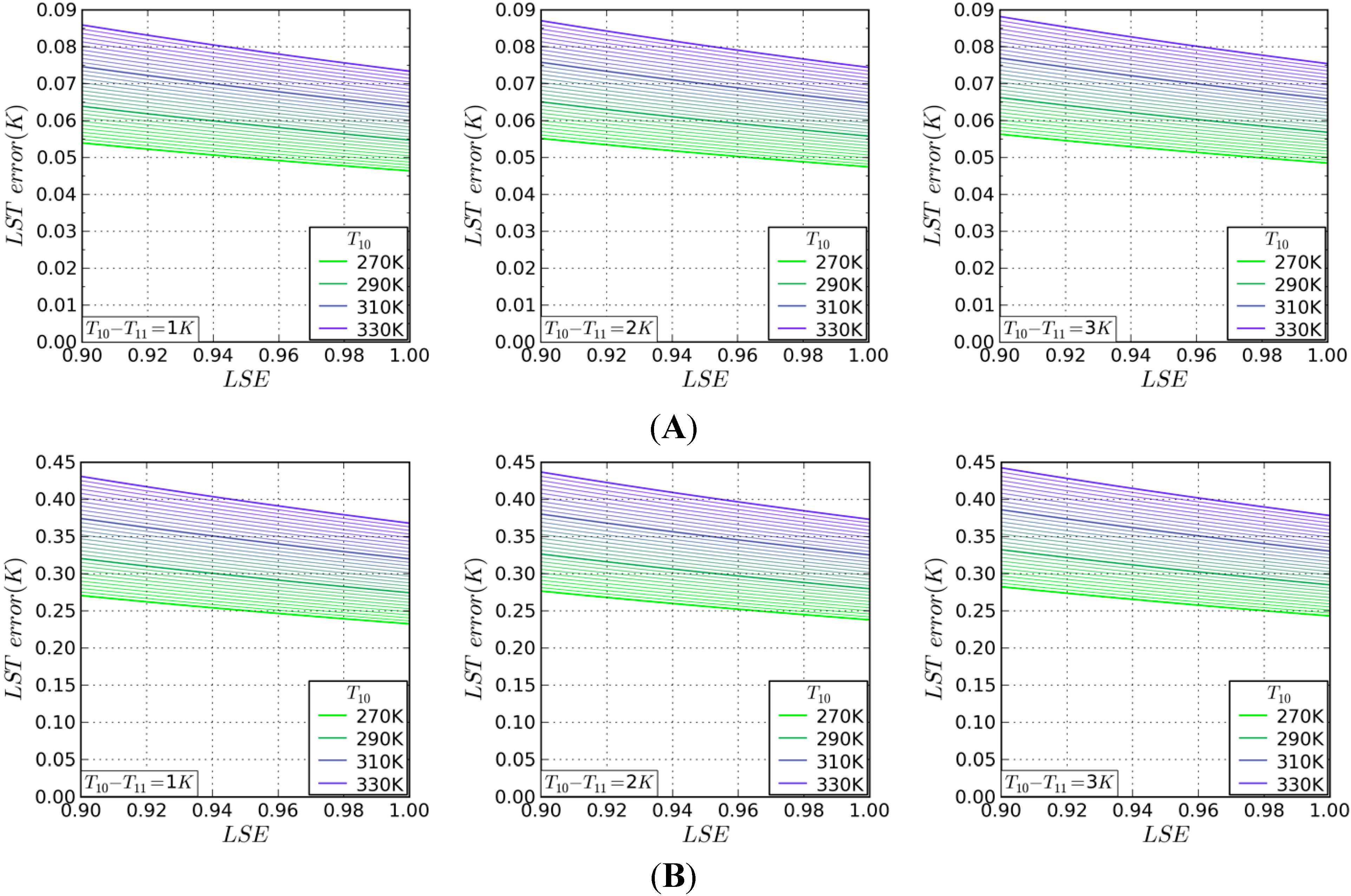
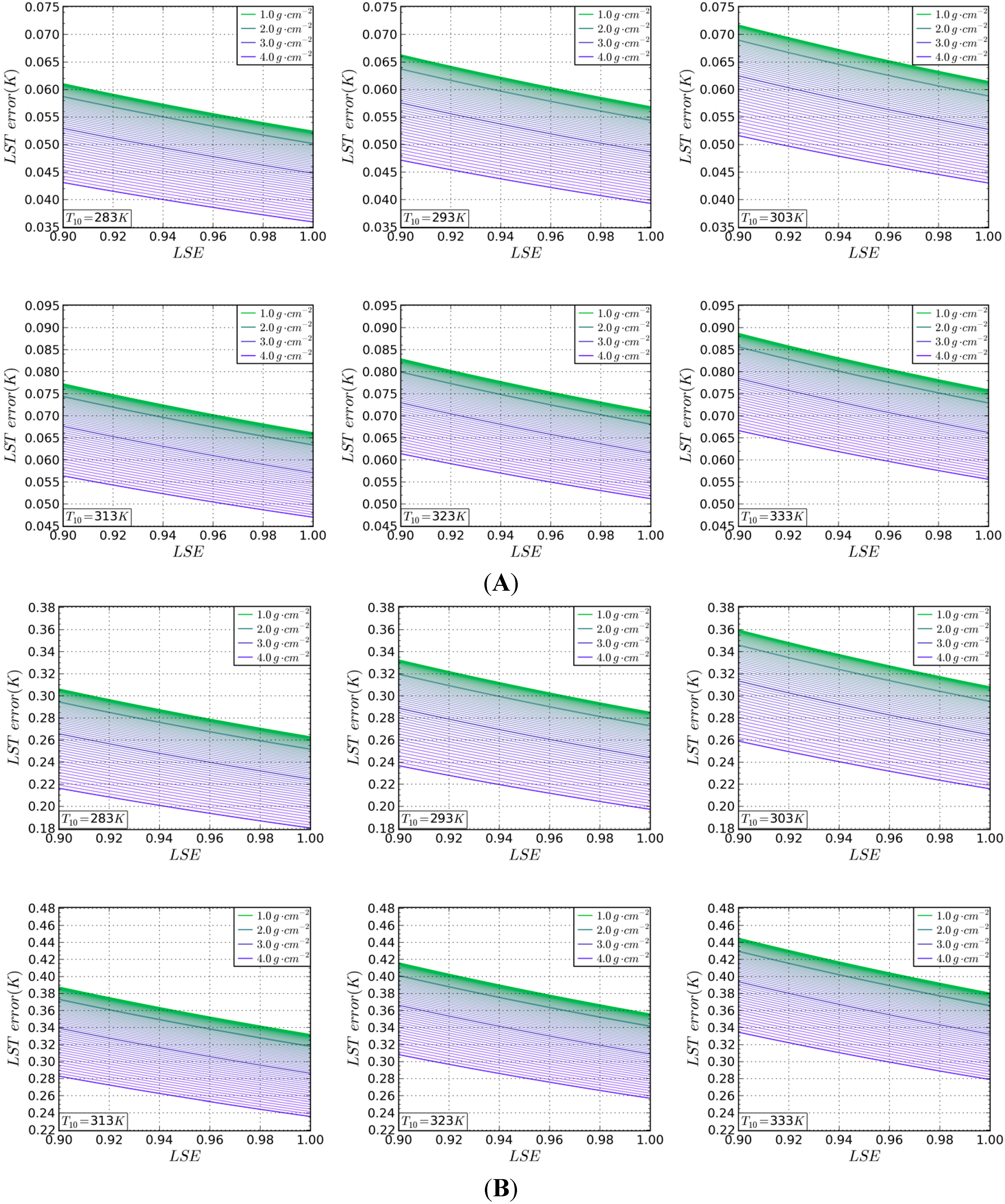
3.1.1. Steadiness Analysis of Atmospheric Transmittance

The atmospheric transmittance is estimated from the water vapour content of the atmosphere. The impact of misestimating the input parameter of the atmosphere transmittance can be assessed by the water vapour content in the column, which is taken to be an important input parameter for the SWA. Because the LST error is related to the brightness temperatures of band10 and band11, we set T10 = 283.0–333.0 K, with an interval of 10.0 K, for a T10–T11 difference of −3–3 K to calculate the LST estimation error, assuming e10 = 0.967 and e11 = 0.971 and undervaluing the atmospheric water vapour content by 0.1 and 0.2 g·cm−2, as was done by Rozenstein et al. (2014) The water vapour content range was 1.0–4.0 g·cm−2.
The LST estimation error is large when the atmospheric water vapour content is 4.0 g·cm−2 and T10 is 3 K lower than T11. In addition, for constant values of the other parameters, higher T10 values correlate with higher LST errors. The specific error variation is shown in Figure 2A,B. In the case of underestimating the water vapour content by 0.1 g·cm−2 and 0.2 g·cm−2, the corresponding maximum LST errors are 0.56 K and 1.11 K, respectively, and the RMSEs of the LST error are 0.30 K and 0.59 K, respectively. The contribution of the calculated atmospheric transmittance error to the retrieved LST is not only related to the water vapour content but also correlates with the LSEs of band10 and band11. The ratio of the LSEs of band10 and band11 is invariant in the analysis process. When the water vapour content column is undervalued by 0.1 and 0.2 g·cm−2, the corresponding maximum LST errors are 0.21 K and 0.41 K, respectively, and the RMSEs of the LST error are 0.10 K and 0.19 K, respectively, as illustrated in Figure 3A,B.
Figure 2. (A) The LST evaluated error (K) in the case of undervaluing the atmospheric water vapour content by 0.1 g·cm−2 for a water vapour content in the range of 1.0–4.0 g·cm−2 and an interval of 1.0 g·cm−2 over six gradations of T10 = 283.0–333.0 K and a T10–T11 value range of −3.0–3.0K. e10 = 0.967, and e11 = 0.971. (B) The LST evaluation error (K) for undervaluing the atmospheric water vapour content by 0.2 g·cm−2 under the same conditions as in (A).
Remotesensing 07 04371 g002
Figure 3. The LST evaluation error (K) in the case of undervaluing the atmospheric water vapour content by 0.1 g·cm−2 (A) and 0.2 g·cm−2 (B) for water vapour contents in the range of 1.0–4.0 g·cm−2 at an interval of 1.0 g·cm−2 over six gradations of T10 = 283.0–333.0 K and a T10–T11 value of 1 K. The LSE variable is independent.
Remotesensing 07 04371 g003

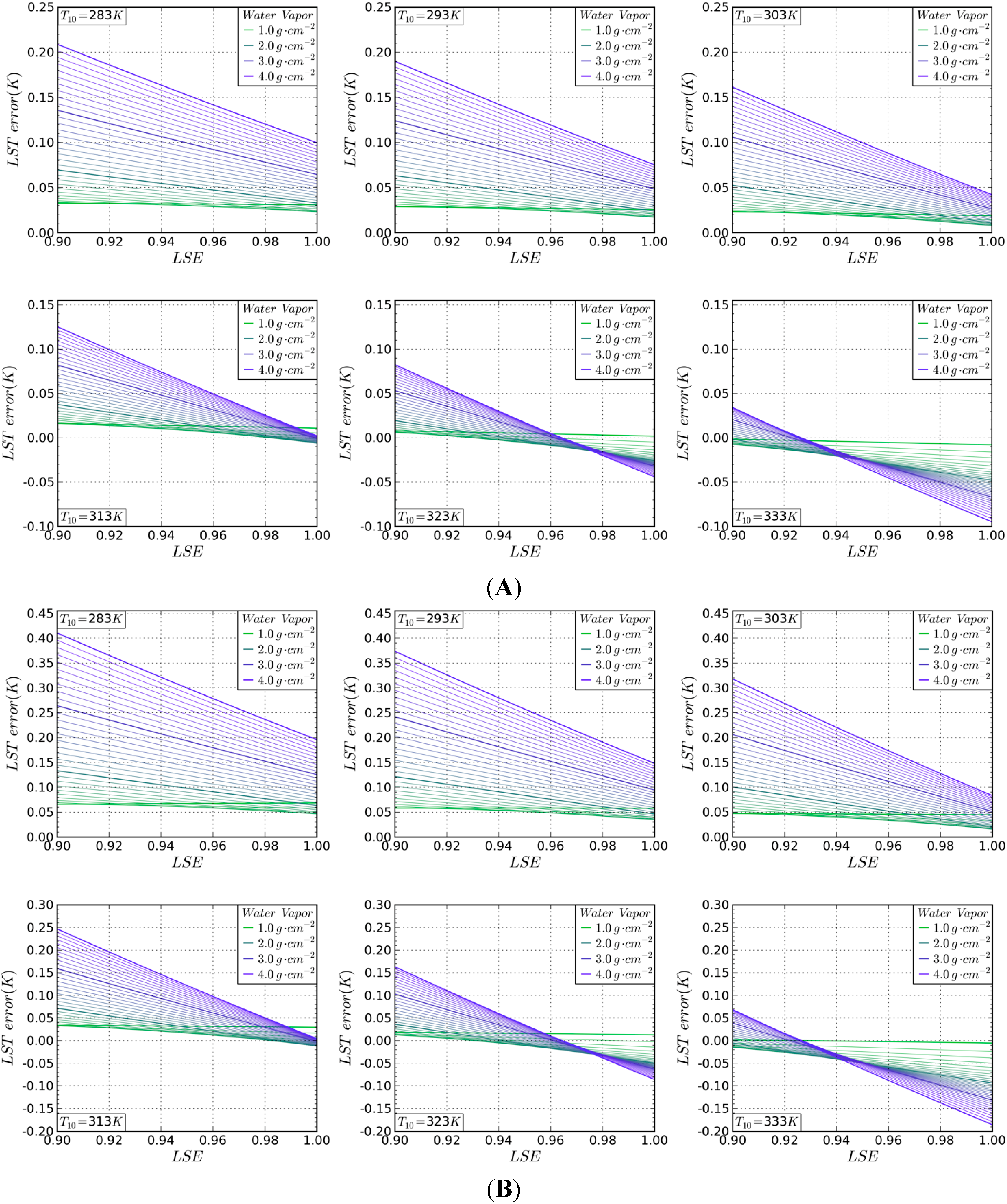
3.1.2. Stability Analysis of LSE

Due to the possibility of having separate LSE errors in both bands, the impact on the LST estimation error of simultaneous errors in the LSE values of both band10 and band11 is discussed in the following. The LSE estimation error also generates an LST calculation error when the atmospheric transmittance has been precisely estimated. In general, the LST calculation error has a positive correlation with the T10 and T10–T11 values and has a negative correlation with LSE, as illustrated in Figure 4A,B. To be specific, the maximum LST calculation error, 0.44 K, occurs when T10 is 330 K, the T10–T11 value is 3 K and the LSE is 0.900 due to undervaluing by 0.005. In the case of underestimating the LSE by 0.001, the maximum LST calculation error is 0.09 K. In Figure 4A,B, the atmospheric water vapour content was kept constant at 1.5 g·cm−2. The sensitivity of the LSE to the LST estimation error was analysed as the atmospheric water vapour content varied from 1.0–4.0 g·cm−2, as seen in Figure 5A,B. The LST calculation error has a positive correlation with the T10 value and has a negative correlation with LSE and water vapour content. The maximum LST calculation error, 0.45 K, occurs when T10 is 333 K, the water vapour content is 1.0 g·cm−2, and LSE is 0.900 due to undervaluing by 0.005.
Generally speaking, the SWA presented in this paper is stable with respect to the impact of incorrectly estimating the LSE and the atmospheric transmittance, i.e., the atmospheric water vapour content. Furthermore, the LST evaluation error is negatively correlated with the LSE estimate.
Figure 4. The illustration of the LST calculation error (K) in the case of undervaluing LSE by 0.001 (A) and 0.005 (B) over four gradations of T10 = 270.0–330.0 K with an interval of 20 K. The atmospheric water vapour content was constant at 1.5 g·cm−2, and the T10–T11 values were 1.0, 2.0, and 3.0 K. The LSE variable is independent.
Remotesensing 07 04371 g004
Figure 5. The illustration of the LST calculation error (K) in the case of undervaluing LSE by 0.001 (A); and 0.005 (B) over six gradations of T10 = 283.0–333.0 K with an interval of 10.0 K. The atmospheric water vapour content varies in the range of 1.0–4.0 g·cm−2 with an interval of 1.0 g·cm−2, and the T10–T11 value is 1.0 K. The LSE variable is independent.
Remotesensing 07 04371 g005

3.2. Evaluation of the Accuracy of the Proposed SWA

MODTRAN 4.0 was used to simulate a series of thermal radiation processes from the ground to the sensor based on the Mid-Latitude Summer atmospheric profile with specified LST, LSE and water vapour content values to evaluate the accuracy of the SWA. First, the simulated thermal radiance values were converted to brightness temperatures corresponding to the Landsat-8 TIRS, band10 and band11, as Ti input parameters for the SWA. Then, according to our SWA and the given input parameters, the LST was calculated. Finally, the LST evaluation errors were obtained by calculating the difference between the given and calculated LSTs. The 90 combination scenes are listed in Table 6. The water vapour content values were 1.0, 2.0, or 3.0 g·cm−2, the range of the assumed LST values was 10–60 °C, with an interval of 10.0 °C, and the range of the LSE values was 0.940–0.980, with an interval of 0.010. The accuracy assessment results, shown in Table 7, are satisfactory, and the RMSE of the LST estimation errors is 0.51 °C, outperforming the result of 0.93 °C from Rozenstein et al. (2014). To assess the general applicability of this SWA to different atmospheric conditions, we also evaluated the accuracy of this SWA under a tropical model and 1976 US standard atmospheric conditions. The assessment results are listed in Table 8 and Table 9. The RMSEs of the LST errors under the tropical model and the 1976 US standard atmospheric conditions are 0.70 °C and 0.63 °C, respectively.
Table 7. Estimation errors of LST for different simulated combinations of specified LST, LSE, and water vapour content values based on the Mid-Latitude Summer atmospheric profile.
Water Vapour Content (g·cm−2)LST (°C)LSE = 0.980LSE = 0.970LSE = 0.960LSE = 0.950LSE = 0.940
1100.37100.36410.35610.34920.3413
200.33840.33020.32200.31380.3056
300.39930.39140.39210.36910.3700
400.53390.53480.52210.52320.5103
500.73600.73500.72680.71860.7178
600.99330.98700.99260.98640.9731
2100.32350.28680.25500.22310.1897
200.28350.26050.22380.20070.1635
300.33880.32500.28330.25860.2450
400.48100.46710.43740.40750.3936
500.69350.66820.65200.62640.6102
600.95150.92780.91770.89390.8611
3100.15320.0701−0.0164−0.1170−0.2146
200.14560.0527−0.0281−0.1099−0.1927
300.21040.13900.0603−0.0194−0.0933
400.36840.28650.22270.13880.0734
500.57080.50590.44030.37390.3067
600.81900.77160.70730.64230.5933
Table 8. Estimation errors of LST for different simulated combinations of specified LST, LSE, and water vapour content values based on the Tropical model atmospheric profile, RMSE = 0.70 °C.
Water Vapour Content (g·cm−2)LST (°C)LSE = 0.980LSE = 0.960LSE = 0.940
1.0200.31300.29580.2766
400.54760.53260.5163
601.03711.02501.0122
2.0200.30780.24150.1730
400.58450.52820.4723
601.11761.07131.0220
3.0200.22810.0416−0.1486
400.60800.45000.2914
601.23131.09580.9587
Table 9. Estimation errors of LST for different simulated combinations of specified LST, LSE, and water vapour content values based on the 1976 US Standard atmospheric profile, RMSE = 0.63 °C.
Water Vapour Content
(g·cm−2)
LST (°C)LSE = 0.980LSE = 0.960LSE = 0.940
1.0200.38930.38360.3762
400.55630.55110.5439
600.99960.99400.9893
2.0200.31290.27040.2288
400.45760.42060.3851
600.87390.84400.8145
3.0200.27490.1358−0.0071
400.55000.43100.3118
601.08490.98230.8787

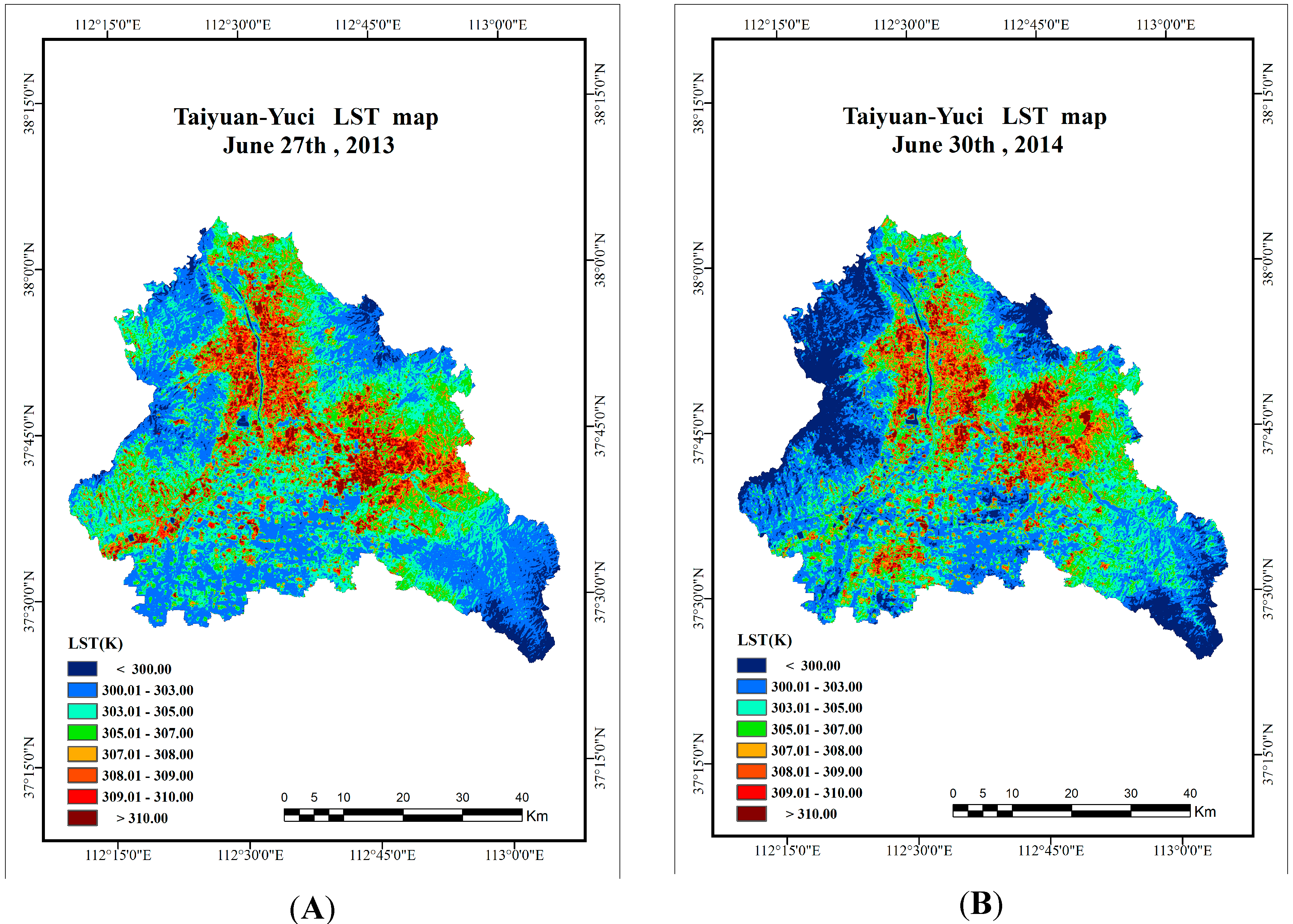
4. A Case Study of an Urban Area in China

4.1. Study Area

The city of Taiyuan-Yuci, China, was chosen as the urban study area. This urban area is located in north-central China, between 37°24'–38°04'N and 112°09'–113°06'E. Taiyuan-Yuci covers a land area of 3336 km2 and has approximately 4.41 million inhabitants (China, the data of the Sixth Population Census, 2010). The region features a warm continental monsoon climate.

4.2. Data Used

Two cloud-free Landsat-8 images, acquired at UTC 03:08:38 on June 27, 2013 and UTC 03:06:26 on June 30, 2014, were rectified to a Universal Transverse Mercator (UTM) projection with WGS-84 datum and UTM zone 49. Two daytime MODIS-Terra images acquired at 02:35 and 04:10 on June 27, 2013 and June 30, 2014, respectively, are also used in this paper to calculate the water vapour content of the atmosphere. Because the MODIS and Landsat-8 acquisition times on the same day were not rigidly consistent, we used the average value of the two temporal MODIS water vapour content estimates to calculate the water vapour content of the atmosphere when the Landsat-8 satellite passed over the study area.
Figure 6. Workflow for retrieving LST from Landsat-8 data.
Remotesensing 07 04371 g006

4.3. LST Retrieval

Using the SWA proposed in this paper, the LST of the urban area was retrieved via the workflow shown in Figure 6. Three sets of input parameters, B 10 ( T 10 ) and B 11 ( T 11 ) , τ 10 and τ 11 , and ε 10 and ε 11 , need to be calculated. The spectral radiance values, B 10 ( T 10 ) and B 11 ( T 11 ) , can be computed from the brightness temperatures T 10 and T 11 using Planck’s radiance function. The atmospheric water vapour content images were produced by using the MOD021KM datasets in conjunction with Equation (13). The obtained water vapour images were then resampled to 30 m × 30 m in accordance with the daytime Landsat-8 images. According to the cubic fit functions of the atmospheric transmittance and water vapour content, the atmospheric transmittance values, τ 10 and τ 11 , were confirmed. Using Landsat-8 OLI datasets, NDVI images were retrieved. The LSE, ε 10 and ε 11 can be confirmed with the NDVI images and Equations (14) and (15), and the emissivity values are listed in Table 6. The three input parameters have now all been confirmed and entered into the SWA formula, and the LST images have been produced. Figure 7 shows the LST estimated from the Landsat-8 TIR data. The LST on June 27, 2013, ranges from 296.6 K–323.8 K, with a mean value of 304.5 K and a standard deviation of 2.953 K. The LST on June 30, 2014, ranges from 292.4 K–322.9 K, with a mean value of 303.7 K and a standard deviation of 3.490 K.
Figure 7. The LST Spatial distribution of the study urban area retrieved from Landsat-8: (A) on June 27, 2013, and (B) on June 30, 2014.
Remotesensing 07 04371 g007

5. Conclusions

A practical SWA for Landsat-8 TIRS data was proposed in this paper. The analysis of sensitivity shows that the SWA has good stability. In five sensitivity analysis scenarios using the Mid-Latitude Summer atmospheric profile, the minimum LST error is −0.839 K, and the maximum LST error is 0.786 K. In general, the LST error is very sensitive when the water vapour content and T10–T11 change together, as is seen in Figure 2B, especially when the water vapour content is 0.5–1.0 g·cm−2. Based on the validation results of the simulation data generated by MODTRAN 4.0, the SWA performs very well. The verification result is satisfactory in that the maximum and minimum LST errors are 0.993 K and 0.016 K, respectively, and the LST error RMSE is 0.51 K under Mid-Latitude Summer atmospheric conditions. The LST error RMSEs under Tropical and 1976 US standard atmospheric conditions are 0.70 K and 0.63 K, respectively. The assessment results demonstrate that the SWA is not only steady and accurate but also universal for different atmospheric conditions.
In this paper, we offer a strategy for evaluating the atmospheric water vapour content using MODIS data and for determining the relationship between the atmospheric transmissivity and water vapour content from Landsat-8 TIRS data using simulation data from MODTRAN 4. An exploratory attempt was performed on a corresponding LSE estimation based on Landsat-8 TIRS data, presented by the LSE of three classic earth surfaces and one new earth surface (galvanized coloured roofs), which further improved the SWA’s integrality and practicality. Additionally, a complete application was performed by retrieving the LST of a study area. The proposed SWA in this paper will contribute to the completion of the inversion algorithm system of LST and will promote the application of remote sensing technology in the research of the thermal environment of the Earth.

Acknowledgements

This study was supported by the Natural Science Foundation for the Youth Program of China (Program No. 51308370), The authors are grateful to the anonymous reviewers whose constructive suggestions have greatly improved the quality of our manuscript and are also grateful to the MODIS, ASTER and Landsat-8 science teams for their excellent and accessible data products. We would like to thank all the project partners and members for their support.

Author Contributions

All authors contributed significantly to this manuscript. The specific contributions include data collection (Meijun Jin, Junming Li and Caili Wang), data processing (Meijun Jin and Ruilan Shang), conceiving the idea and designing the methodology (Junming Li and Meijun Jin), and manuscript writing (Meijun Jin, Junming Li and Caili Wang).

Conflicts of Interest

The authors declare no conflict of interest.

References and Notes

  1. Chapin, F.; Sturm, M.; Serreze, M.; McFadden, J.; Key, J.; Lloyd, A.; McGuire, A.; Rupp, T.; Lynch, A.; Schimel, J. Role of Land-Surface Changes in Arctic Summer Warming. Science 2005, 310, 657–660. [Google Scholar] [CrossRef] [PubMed]
  2. Kalnay, E.; Cai, M. Impact of urbanization and land-use change on climate. Nature 2003, 423, 528–531. [Google Scholar] [CrossRef] [PubMed]
  3. Ramanathan, V.; Crutzen, P.; Kiehl, J.; Rosenfeld, D. Aerosols, climate, and the hydrological cycle. Science 2001, 294, 2119–2124. [Google Scholar] [CrossRef]
  4. Wan, Z.; Wang, P.; Li, X. Using MODIS land surface temperature and normalized difference vegetation index products for monitoring drought in the Southern Great Plains, USA. Int. J. Remote Sens. 2004, 25, 61–72. [Google Scholar] [CrossRef]
  5. Gallo, K.P.; Owen, T.W. Assessment of urban heat island: A multi-sensor perspective for the Dallas-Ft. Worth, USA region. Geocarto. Int. 1998, 13, 35–41. [Google Scholar] [CrossRef]
  6. Streutker, D.R. A remote sensing study of the urban heat island of Houston, Texas. Int. J. Remote Sens. 2002, 23, 2595–2608. [Google Scholar] [CrossRef]
  7. Weng, Q. A Remote sensing-GIS evaluation of urban expansion and its impact on surface temperature in the Zhujiang Delta, China. Int. J. Remote Sens. 2001, 22, 1999–2014. [Google Scholar]
  8. Chen, X.L.; Zhao, H.; Li, P.; Yin, Z. Remote sensing image-based analysis of the relationship between urban heat island and land use/cover changes. Remote Sens. Environ. 2002, 104, 133–146. [Google Scholar] [CrossRef]
  9. Yuan, F.; Bauer, M.E. Comparison of impervious surface area and Normalized Difference Vegetation Index as indicators of surface urban heat island effects in Landsat imagery. Remote Sens. Environ. 2007, 106, 375–386. [Google Scholar] [CrossRef]
  10. Rozenstein, O.; Qin, Z.; Derimian, Y.; Karnieli, A. Derivation of land surface temperature for Landsat-8 TIRS using a split window algorithm. Sensors 2014, 14, 5768–5780. [Google Scholar] [CrossRef] [PubMed]
  11. Li, Z.L.; Tang, B.H.; Wu, H.; Ren, H.; Yan, G.; Wan, Z.; Trigo, I.F.; Sobrino, J.A. Satellite-derived land surface temperature: Current status and perspectives. Remote Sens. Environ. 2013, 131, 14–37. [Google Scholar] [CrossRef]
  12. Li, Z.L.; Zhang, R.; Sun, X.; Su, H.; Tang, X.; Zhu, Z. Experimental system for the study of the directional thermal emission of natural surfaces. Int. J. Remote Sens. 2004, 25, 195–204. [Google Scholar] [CrossRef]
  13. Ottlé, C.; Vidal-Madjar, D. Estimation of land surface temperature with NOAA9 data. Remote Sens. Environ. 1992, 40, 27–41. [Google Scholar] [CrossRef]
  14. Price, J.C. Estimating surface temperatures from satellite thermal infrared data—A simple formulation for the atmospheric effect. Remote Sens. Environ. 1983, 13, 353–361. [Google Scholar] [CrossRef]
  15. Price, J.C. Land surface temperature measurements from the split window channels of the NOAA 7 AVHRR. J. Geophys. Res. 1984, 89, 7231–7237. [Google Scholar] [CrossRef]
  16. Becker, F. The impact of spectral emissivity on the measurement of land surface temperature from a satellite. Int. J. Remote Sens. 1987, 8, 1509–1522. [Google Scholar] [CrossRef]
  17. Becker, F.; Li, Z.L. Towards a local split window method over land surfaces. Int. J. Remote Sens. 1990, 11, 369–393. [Google Scholar] [CrossRef]
  18. Sobrino, J.A.; Coll, C.; Caselles, V. Atmospheric correction for land surface temperature using NOAA-11 AVHRR Channels 4 and 5. Remote Sens. Environ. 1991, 38, 19–34. [Google Scholar] [CrossRef]
  19. Coll, C.; Caselles, V.; Sobrino, J.A.; Valor, E. On the atmospheric dependence of the split-window equation for land surface temperature. Int. J. Remote Sens. 1994, 15, 105–122. [Google Scholar] [CrossRef]
  20. Sobrino, J.A.; Li, Z.L.; Stoll, M.P.; Becker, F. Improvements in the split-window technique for land surface temperature determination. IEEE Trans. Geosci. Remote Sens. 1994, 32, 243–253. [Google Scholar] [CrossRef]
  21. Prata, A.J. Land surface temperature determination from satellites. Adv. Space Res. 1994, 14, 15–26. [Google Scholar] [CrossRef]
  22. Ulivieri, C.; Castronuovo, M.M.; Francioni, R.; Cardillo, A. A split window algorithm for estimating land surface temperature from satellites. Adv. Space Res. 1994, 14, 59–65. [Google Scholar] [CrossRef]
  23. Wan, Z.; Dozier, J. A generalized split-window algorithm for retrieving land-surface temperature from space. IEEE Geosci. Remote Sens. 1996, 34, 892–905. [Google Scholar] [CrossRef]
  24. Sobrino, J.A.; Li, Z.L.; Stoll, M.P.; Becker, F. Multi-channel and multi-angle algorithms for estimating sea and land surface temperature with ATSR data. Int. J. Remote Sens. 1996, 17, 2089–2114. [Google Scholar] [CrossRef]
  25. Tang, B.H.; Li, Z.L. Retrieval of land surface bidirectional reflectivity in the mid-infrared from MODIS Channels 22 and 23. Int. J. Remote Sens. 2008, 29, 4907–4925. [Google Scholar] [CrossRef]
  26. Atitar, M.; Sobrino, J.A. A split-window algorithm for estimating LST from Meteosat 9 Data: Test and comparison with in situ data and MODIS LSTs. IEEE Geosci. Remote Sens. 2009, 6, 122–126. [Google Scholar] [CrossRef]
  27. Mao, K.; Qin, Z.; Shi, J.; Gong, P. A practical split-window algorithm for retrieving land-surface temperature from MODIS data. Int. J. Remote Sens. 2005, 26, 3181–3204. [Google Scholar] [CrossRef]
  28. Chédin, A.; Scott, N.A.; Berroir, A. A single-channel, double-viewing angle method for sea surface temperature determination from coincident Meteosat and TIROS-N radiometric measurements. J. Appl. Meteorol. 1982, 21, 613–618. [Google Scholar] [CrossRef]
  29. Prata, A.J. Surface temperatures derived from the Advanced Very High Resolution Radiometer and the Along Track Scanning Radiometer. 1. Theory. J. Geophys. Res. 1993, 98, 16689–16702. [Google Scholar] [CrossRef]
  30. Prata, A.J. Land surface temperatures derived from the Advanced Very High Resolution Radiometer and the Along-Track Scanning Radiometer 2. Experimental results and validation of AVHRR algorithms. J. Geophys. Res. 1994, 99, 13025–13058. [Google Scholar] [CrossRef]
  31. Li, Z.L.; Stoll, M.P.; Zhang, R.H.; Jia, L.; Su, Z.B. On the separate retrieval of soil and vegetation temperatures from ATSR data. Sci. China Series D: Earth Sci. 2001, 44, 97–111. [Google Scholar] [CrossRef]
  32. Sobrino, J.A.; Romaguera, M. Land surface temperature retrieval from MSG1-SEVIRI data. Remote Sens. Environ. 2004, 92, 247–254. [Google Scholar] [CrossRef]
  33. Irons, J.R.; Dwyer, J.L.; Barsi, J.A. The next Landsat satellite: The Landsat Data Continuity Mission. Remote Sens. Environ. 2012, 122, 11–21. [Google Scholar] [CrossRef]
  34. Cuenca, R.H.; Ciotti, S.P.; Hagimoto, Y. Application of Landsat to evaluate effects of irrigation forbearance. Remote Sens. 2013, 5, 3776–3802. [Google Scholar] [CrossRef]
  35. Jimenez-Munoz, J.C.; Sobrino, J.A.; Skokovic, D.; Matter, C.; Cristobal, J. Land surface temperature retrieval methods from Landsat-8 Thermal Infrared Sensor data. IEEE Geosci. Remote Sens. 2014, 11, 1840–1843. [Google Scholar] [CrossRef]
  36. Du, C.; Ren, H.Z.; Qin, Q.M.; Meng, J.J.; Li, J. Split-window algorithm For estimating land surface temperature from Landsat 8 TIRs data. In Proceedings of 2014 IEEE International Geoscience and Remote Sensing Symposium (IGARSS), Quebec City, QC, Canada, 13–18 July 2014; pp. 3578–3581.
  37. Rybicki, G.B.; Lightman, A.P. Fundamental of Radiative Transfer. Radiative Processes in Astrophysics; John Wiley & Sons, Inc.: New York, NY, USA, 1979. [Google Scholar]
  38. Ottle, C.; Stoll, M. Effect of atmospheric absorption and surface emissivity on the determination of land surface temperature from infrared satellite data. Int. J. Remote Sens. 1993, 14, 2025–2037. [Google Scholar] [CrossRef]
  39. Qin, Z.; Karnieli, A. A Mono-Window Algorithm for Retrieving Land Surface Temperature from Landsat TM Data and Its Application to the Israel-Egypt Border Region. Int. J. Remote Sens. 2001, 22, 3722–3723. [Google Scholar]
  40. Jiménez-MuÌoz, J.C.; Sobrino, J.A. A generalized single 2 channel method for retrieving land surface temperature from remote sensing Data. J. Geophys. Res. 2003, 8. [Google Scholar] [CrossRef]
  41. Qin, Z.; Dall’Olmo, G.; Karnieli, A.; Berliner, P. Derivation of split window algorithm and its sensitivity analysis for retrieving land surface temperature from NOAA-Advanced very High Resolution Radiometer data. Geophys. Res. Atmos. 2001, 106, 22655–22670. [Google Scholar] [CrossRef]
  42. Kaufmann, Y.J.; Gao, B.C. Remote sensing of water in the Near IR from EOS/MODIS. IEEE Trans. Geosci. Remote Sens. 1992, 30, 871–884. [Google Scholar] [CrossRef]
  43. Sobrino, J.A.; Raissouni, N.; Li, Z.L. A comparative study of land surface emissivity retrieval from NOAA data. Remote Sens. Environ. 2001, 75, 256–266. [Google Scholar] [CrossRef]
  44. Aster Spectral Library. Available online: http://speclib.jpl.nasa.gov/ (accessed on 4 June 2014).
  45. Carlson, T.N.; Ripley, D.A. On the relation between NDVI, fractional vegetation cover, and leaf area index. Remote Sens. Environ. 1997, 62, 241–252. [Google Scholar] [CrossRef]
  46. Sobrino, J.A.; Jiménez-Muñoz, J.C.; Paolini, L. Land surface temperature retrieval from LANDSAT TM 5. Remote Sens. Environ. 2004, 90, 434–440. [Google Scholar] [CrossRef]
  47. Sobrino, J.A.; Raissouni, N. Toward remote sensing methods for land cover dynamic monitoring: Application to Morocco. Int. J. Remote Sens. 2000, 21, 353–366. [Google Scholar] [CrossRef]
  48. Sobrino, J.A.; Caselles, V.; Becker, F. Significance of the remotely sensed thermal infrared measurements obtained over a citrus orchard. Photogramm. Eng. Remote Sens. 1990, 44, 343–354. [Google Scholar] [CrossRef]

