Article

Toward the Estimation of Surface Soil Moisture Content Using Geostationary Satellite Data over Sparsely Vegetated Area

1
College of Resources and Environment, University of Chinese Academy of Sciences, Beijing 100049, China
2
ICube, UdS, CNRS, Boulevard Sebastien Brant, CS10413, Illkirch 67412, France
3
Key Laboratory of Agri-Informatics, Ministry of Agriculture/Institute of Agricultural Resources and Regional Planning, Chinese Academy of Agricultural Sciences, Beijing 100081, China
*
Author to whom correspondence should be addressed.
Remote Sens. 2015, 7(4), 4112-4138; https://doi.org/10.3390/rs70404112
Submission received: 10 November 2014 / Revised: 4 February 2015 / Accepted: 24 March 2015 / Published: 7 April 2015
(This article belongs to the Special Issue Recent Advances in Thermal Infrared Remote Sensing)

Abstract

:
Based on a novel bare surface soil moisture (SSM) retrieval model developed from the synergistic use of the diurnal cycles of land surface temperature (LST) and net surface shortwave radiation (NSSR) (Leng et al. 2014. “Bare Surface Soil Moisture Retrieval from the Synergistic Use of Optical and Thermal Infrared Data”. International Journal of Remote Sensing 35: 988–1003.), this paper mainly investigated the model’s capability to estimate SSM using geostationary satellite observations over vegetated area. Results from the simulated data primarily indicated that the previous bare SSM retrieval model is capable of estimating SSM in the low vegetation cover condition with fractional vegetation cover (FVC) ranging from 0 to 0.3. In total, the simulated data from the Common Land Model (CoLM) on 151 cloud-free days at three FLUXNET sites that with different climate patterns were used to describe SSM estimates with different underlying surfaces. The results showed a strong correlation between the estimated SSM and the simulated values, with a mean Root Mean Square Error (RMSE) of 0.028 m3·m−3 and a coefficient of determination (R2) of 0.869. Moreover, diurnal cycles of LST and NSSR derived from the Meteosat Second Generation (MSG) satellite data on 59 cloud-free days were utilized to estimate SSM in the REMEDHUS soil moisture network (Spain). In particular, determination of the model coefficients synchronously using satellite observations and SSM measurements was explored in detail in the cases where meteorological data were not available. A preliminary validation was implemented to verify the MSG pixel average SSM in the REMEDHUS area with the average SSM calculated from the site measurements. The results revealed a significant R2 of 0.595 and an RMSE of 0.021 m3·m−3.

Graphical Abstract

1. Introduction

The water held in the top few centimeters of the soil, namely surface soil moisture (SSM), is an essential land surface variable because it determines the partitioning of energy at the surface and consequently impacts the associated water and energy fluxes especially over low vegetated conditions [1,2]. The SSM always plays a considerable role in various hydrological models [3,4], meteorological studies [5,6] and ecological applications [7,8]. It is also a fundamental parameter in many other domains, such as the agricultural process [9,10] and carbon/nitrogen cycles [11,12]. Traditional methods usually set up various dense in situ networks for monitoring soil moisture with Time-Domain Reflectometry (TDR) or Frequency-Domain Reflectometry (FDR). Although the in situ network is the most accurate way to obtain soil moisture at present, it is expensive and most likely limited in representing the spatial distribution of soil moisture due to the heterogeneity of the underlying surface.
Remote sensing offers a potential alternative for characterizing the distribution and quantity of soil moisture at a variety of scales. With the spatial advantage of remote sensing technology, the observation of SSM or SSM-related surface variables using remotely sensed data has been widely documented with different electromagnetic spectra from the optical to the microwave regions [13,14,15,16,17,18,19,20,21,22,23]. In general, backscattering coefficient of the surface can be detected by active microwave remote sensing, and subsequently used to estimate soil moisture. However, most of the present active remote sensing systems for exactly the same configuration usually characterize a relatively long revisit time, which is not sufficient for global soil moisture monitoring products. Although the Advanced Scattermeter (ASCAT) is capable of providing soil moisture product with a temporal resolution of 2–3 days, it is merely the value from 0 to 100 representing the extremely dry to extremely wet conditions, rather than the real volumetric water content that is more expected in the aforementioned areas. Compared to active microwave remote sensing, passive microwave remote sensing has shown great potential in the monitoring of SSM through the past Advanced Microwave Scanning Radiometer-Earth Observing System (AMSR-E) to the present Soil Moisture and Ocean Salinity (SMOS), as well as in the upcoming Soil Moisture Active-Passive (SMAP), which will be combined with active remote sensing [13,14,15]. However, the coarse spatial resolution of passive microwave (~25–40 km) has greatly restricted its application, especially at the relatively small scale. Similar to the passive microwave remote sensing, the use of optical/thermal infrared remote sensing to obtain SSM information has also received considerable research attention over the last decades because it has an adequate spatial and temporal resolution, one of the most commonly used optical/thermal infrared data are from the Moderate-Resolution Imaging Spectroradiometer (MODIS) that possess the spatial resolution of 1 km. For bare or sparsely vegetated conditions, the thermal inertia or apparent thermal inertia (ATI) that primarily calculated from the optical/thermal infrared bands, were widely recognized as a feasible proxy of soil moisture [24,25,26]. However, the TI (or ATI) is not the quantitative SSM content, and the empirical relationship between TI (or ATI) and SSM content is not unique and varies with the variation of soil texture. Analogously, empirical models to convert the optical/thermal data-derived evaporative fraction (EF) to soil moisture values also generally work better for bare soils and shallowly rooted plant covers [27]. For more vegetated regions, the soil moisture status was usually obtained from some soil moisture related land surface variables, such as the land surface temperature (LST), the vegetation index (VI) and the evapotranspiration (ET), as well as other auxiliary data (e.g., soil texture, SSM measurements and meteorological data). In particular, based on the scatter plot of LST/VI feature space, the Temperature-Vegetation Dryness Index (TVDI) was one of the most commonly used indices to infer soil moisture status [28]. With the optical/thermal infrared information, many other feature spaces and indices were also developed to indicate soil moisture or soil moisture related land surface parameters. Nevertheless, these indices are far from the real moisture content value, and empirical relationships between these indices and soil moisture measurements are usually needed to convert the remotely sensed indices to quantitative SSM content at the regional scale.
Although the optical/thermal infrared remote sensing of soil moisture has a strong physical basis and fine spatial resolution that better satisfies the requirements of various applications, it measures soil moisture indirectly, and these indirect measurements (e.g., ATI, EF and TVDI) usually need to be converted to quantitative soil moisture content using empirical relationships with other auxiliary data, such as ground soil moisture measurements and soil texture information. In a recent study, Leng et al. (2014) reported a novel bare SSM retrieval model from the synergistic use of the diurnal cycles of LST and net surface shortwave radiation (NSSR) [29]. In this SSM retrieval model, diurnal cycles of LST and NSSR (from either ground measurements or simulated data) are used to obtain an elliptical relationship model and further to get the ellipse parameters; besides, the five model coefficients ni (i = 0, 1, 2, 3, 4) for each cloud-free day are acquired from a land surface model simulation. With both the ellipse parameters and model coefficients, quantitative volumetric soil water content for each cloud-free day can be estimated by the SSM retrieval model. Compared with the previous optical/thermal infrared remote sensing of soil moisture, this newly developed SSM retrieval model has several potential advantages. In particular, the SSM retrieval model is capable of estimating the quantitative volumetric soil water content value directly without establishing an empirical relationship between ground SSM measurements and satellite-derived proxies of SSM. Moreover, as the primary input parameters of the SSM retrieval model are derived from the elliptical relationship between the diurnal cycles of LST and NSSR, a few images that are contaminated by clouds or other adverse factors during the daytime will not practically affect the application of the SSM retrieval model. Moreover, this SSM retrieval model is well suited for long-term mapping and monitoring of SSM time series through the use of observations from the geostationary meteorological satellites (generally 48–96 images per day), such as the Meteosat Second Generation (MSG) of Europe, the Feng Yun (FY) of China and the Geostationary Operational Environmental Satellite (GOES) of United States of America (USA). These abilities are possible due to the attention garnered by numerous algorithms and corresponding land surface products derived from the geostationary meteorological satellites that have been developed and thus provided to for research and various applications, especially in the last decade (http:// landsaf.meteo.pt/; http://satellite.cma.gov.cn/portalsite/default.aspx#; http://www.goes.noaa.gov/). However, because the SSM retrieval model was originally developed for bare soils, some of the essential issues remain to be properly addressed before applying the SSM retrieval model to remotely sensed observations. As noted by previous studies [29,30], the two main challenges are taking into account vegetation and determining the five model coefficients ni (i = 0, 1, 2, 3, 4) of the SSM retrieval model for each cloud-free day at a regional scale. On the basis of previous work, this study aims to assess the feasibility of using the SSM retrieval model with geostationary satellite observations in vegetated conditions. In particular, we also attempt to determine the five model coefficients ni (i = 0, 1, 2, 3, 4) synergistically using geostationary satellite observations and SSM measurements in cases where meteorological data are not available for a land surface model simulation to obtain to model coefficients.
This paper is organized as follows. Section 2 details the study area and the dataset involved in the study. Section 3 addresses the methodology. Section 4 mainly deals with the results and analysis. Section 5 concludes the paper.

2. Study Area and Dataset

2.1. FLUXNET Meteorological Data

The FLUXNET is a “network of regional networks” coordinating regional and global analysis of observations from micrometeorological tower sites. At present, over 500 tower sites are operated on a long-term and continuous basis (http://fluxnet.ornl.gov/). The FLUXNET database has been widely used to provide essential inputs for ecology and land surface modeling, as well as to evaluate remote sensing products (e.g., evapotranspiration, energy components and primary productivity). In this study, meteorological data collected at three FLUXNET sites located in USA, namely Bondville, Audubon Research Ranch and Brookings, are used to drive a land surface model to produce simulated data and are subsequently utilized to develop the methodology for the SSM retrieval in vegetated conditions. A detailed description of the three sites is provided in Table 1.
Table 1. A brief description of the Bondville, Audubon Research Ranch and Brookings FLUXNET sites (USA).
SiteSoil TextureLatitude, LongitudeLand UseClimate Type
BondvilleSilty Loam44.0062°N, −88.2904°Wcroplandtemperate continental
Audubon Research RanchSandy Loam31.5907°N, −110.5092°Wdesert grasslandtemperate arid
BrookingsClay Loam44.3453°N, −96.8362°Wrange grasslandhumid continental
Meteorological data, including downward solar radiation, downward longwave radiation, precipitation, air temperature, wind speed, wind direction, atmospheric pressure at the surface and specific humidity with a temporal resolution of 30 min on cloud-free days, are collected at the three sites. In particular, to avoid the freeze/thaw conditions, only the meteorological data from the day of year (DOY) 100 to 300 are considered in the land surface model simulation. In total, eight cloud-free days at the Bondville site during 2001, which has been used in the same way in Leng et al. (2014) to develop the bare SSM retrieval model, are selected to assess the influences of vegetation on the SSM retrieval model [29]. Besides, 66 cloud-free days at the Audubon Research Ranch site and 41 cloud-free days at the Brookings site during 2010, as well as 44 cloud-free days at Bondville site during 2006, have also been selected to create simulated data for further investigation.
Figure 1. Study area of the REMEDHUS soil moisture network. The map shows a false-color Landsat image (bands 4, 3 and 2) of the area.
Remotesensing 07 04112 g001

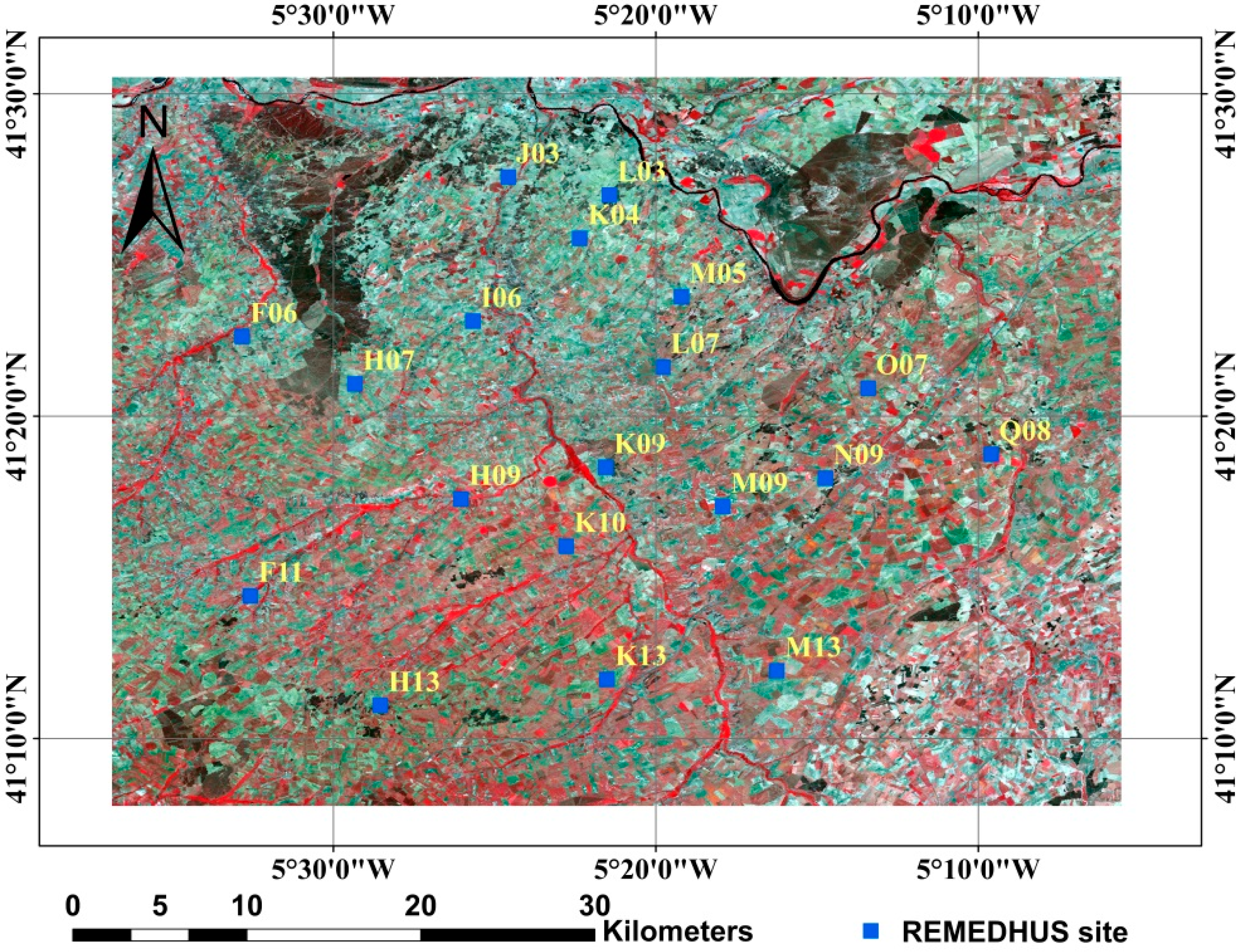
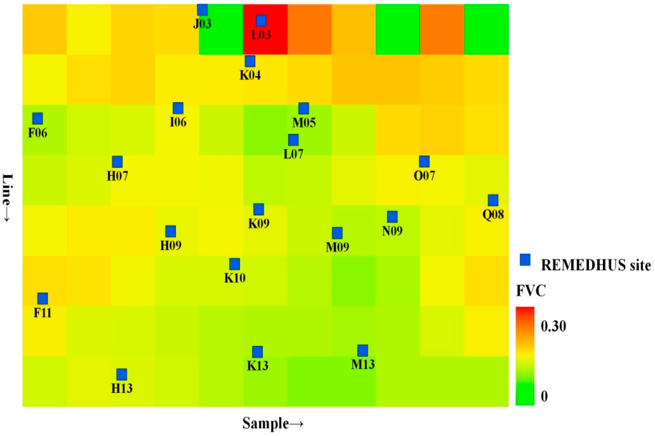
2.2. REMEDHUS Soil Moisture Network

In addition to the FLUXNET data, soil moisture measurements from the REMEDHUS soil moisture network in the semi-arid parts of the Duero Basin (Spain) are also used in this study. The REMEDHUS soil moisture network provides a continuous measurement of soil moisture at a depth of 5 cm each hour. In previous studies, the REMEDHUS soil moisture measurements have been widely used to validate and calibrate several satellite-derived soil moisture products at various scales [31,32,33,34]. Figure 1 depicts the REMEDHUS region, where elevation generally ranges from 700 to 900 m, with a relatively gentle slope (less than 10% slope). The REMEDHUS soil moisture data from 19 available measurement sites during 2010 and 2011 are obtained from the International Soil Moisture Network (ISMN) [35]. The numbers of line and sample for each site in the European portion of the MSG data, together with a detailed description of the REMEDHUS sites, are shown in Table 2. For the soil moisture measurements and soil texture information of the REMEDHUS sites, comprehensive laboratory analyses of soil samples are carried out to calibrate the TDR measurements and to assess the soil properties at each station [33, 36]. According to the numbers of line and sample shown in Table 2, almost all 19 sites take one specific MSG pixel, except for L07 and M05. The soil moisture measurements on cloud-free days in April, July and October of the years 2010 and 2011 at the 19 available sites are selected in this study. In particular, the selected cloud-free days meet the requirement that the MSG observations must be available for all the pixels that are associated with the locations of the 19 measurement sites. Finally, 29 and 30 cloud-free days are selected for the three months in 2010 and 2011, respectively. In this study, because meteorological data collected in the REMEDHUS network fail to meet the requirement to drive the land surface model, the REMEDHUS soil moisture measurements are primarily used to determine the model coefficients of the SSM retrieval model combining with the satellite observations. Moreover, these soil moisture measurements are also conducted to verify the retrieved SSM in the REMEDHUS region.
Table 2. Soil textures and locations of the 19 REMEDHUS soil moisture network sites (Spain). The numbers associated with the line and sample describe the location of each site in the European portion of the Meteosat Second Generation (MSG) data.
SiteSand (%)Silt (%)Clay (%)Latitude, LongitudeLine, Sample
F0667.1913.7019.1141.37455°N, −5.54714°W476, 160
F1181.5211.976.5141.24040°N, −5.54291°W479, 160
H0785.109.645.2641.35004°N, −5.48891°W477, 162
H0919.7844.9935.2341.29050°N, −5.43402°W478, 163
H1370.3611.4518.1941.18381°N, −5.47572°W481, 162
I0689.815.934.2641.38251°N, −5.42786°W476, 163
J0385.0511.263.6941.45703°N, −5.40964°W474, 164
K0487.099.273.6441.42529°N, −5.37267°W475, 165
K0974.3615.0010.6441.30690°N, −5.35925°W478, 165
K1091.165.713.1341.26611°N, −5.37972°W479, 164
K1362.2218.2119.5741.19720°N, −5.35861°W480, 165
L0382.256.4411.3141.44765°N, −5.35734°W474, 165
L0746.8020.7832.4241.35873°N, −5.32977°W476, 166
M0581.648.3110.0541.39508°N, −5.32010°W476, 166
M0949.8324.8925.2841.28662°N, −5.29868°W478, 167
M133.5732.0464.3941.20170°N, −5.27085°W480, 167
N0962.4616.7820.7641.30126°N, −5.24569°W478, 168
O0778.8413.477.6941.34778°N, −5.22361°W477, 169
Q0886.075.688.2541.31359°N, −5.16005°W477, 170

2.3. Satellite Observations

The MSG is a new multi-spectral and multi-temporal geostationary satellite developed by the European Space Agency (ESA) and the European Meteorological Satellite Organization (EUMETSAT). The satellite has an image-repeat cycle of 15 min. Its main payload is the Spinning Enhanced Visible and Infrared Imager (SEVIRI), which features unique spectral characteristics and accuracy, with a 3 km resolution (sampling distance) at nadir (1 km for the high-resolution visible channel), and 12 spectral channels [37]. At present, several land surface products have been developed and provided by the EUMETSAT. In this paper, MSG products, including the LST, the Down-Welling Surface Shortwave Flux (DSSF) and land surface albedo on the 59 selected cloud-free days associated with the REMEDHUS soil moisture measurements in 2010 and 2011, are obtained from the Land Surface Analysis-Satellite Applications Facility (LSA-SAF) [38]. In particular, the DSSF and daily land surface albedo products are used to calculate NSSR, and the diurnal cycles of LST and NSSR with the same temporal resolution (30 min) are utilized to describe an elliptical relationship and further to derive the ellipse parameters.

3. Methodology

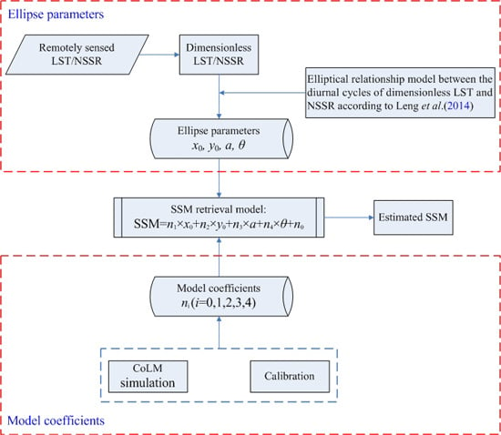
3.1. Overview of the Previous Bare Surface Soil Moisture (SSM) Retrieval Model

Based on the fact that diurnal cycles of LST and NSSR can be described as cosine functions of time during the daytime on the cloud-free days, Leng et al. (2014) derive an elliptical relationship between LST and NSSR, which can be expressed as [29]:
p 2 2 ( x q 1 ) 2 2 p 1 p 2 [ cos ( β Δ t ) ] ( x q 1 ) ( y q 2 ) + p 1 2 ( y q 2 ) 2 = [ p 1 p 2 sin ( β Δ t ) ] 2
where x and y are the dimensionless LST and NSSR, respectively, β is the width of the half-period of the cosine term, Δ t is the difference between maximum LST time and maximum NSSR time, p 1 , q 1 , p 2 and q 2 are parameters of diurnal LST and NSSR cycles. In general, soil moisture mainly affects the soil temperature variation through the thermal inertia for a particular soil texture under a given atmospheric condition. While for NSSR, soil moisture has a significant effect on bare surface albedo which will greatly govern the diurnal cycle of NSSR. Namely, each combination of soil texture and soil moisture will correspond to particular temporal variations of LST and NSSR under a given cloud-free day. Hence, the parameters ( p 1 , q 1 , p 2 , q 2 , β and Δ t ) that describe the diurnal LST and NSSR cycles are constants for a given soil texture and soil moisture condition, and will also vary differently in conditions that the bare surface is with various soil textures and soil moisture status. Based on the elliptical relationship between diurnal cycles of LST and NSSR for cloud-free days, the five ellipse parameters, including the center horizontal coordinate (x0), the center vertical coordinate (y0), the semi-major axis (a), the semi-minor axis (b) and the rotation angle (θ) can be calculated as:
{ x 0 = q 1 y 0 = q 2 θ = 1 2 cot 1 [ p 1 2 p 2 2 2 p 1 p 2 cos ( β Δ t ) ] a = p 1 sin ( β Δ t ) b = p 2 sin ( β Δ t )
Because the ellipse parameters are affected directly by SSM conditions and soil textures for a given atmospheric condition, a stepwise regression method is used to determine the parameters for SSM retrieval. With the simulated data for eight cloud-free days, it is found that the four ellipse parameters (θ, y0, a, x0) are most significant for the estimation of SSM. The newly developed bare SSM retrieval model is written as follows:
S S M = n 1 × x 0 + n 2 × y 0 + n 3 × a + n 4 × θ + n 0
where S S M is the daily average SSM (m3·m−3); x0, y0, a and θ are the ellipse parameters of the elliptical relationship between diurnal LST and NSSR cycles and represent the ellipse center horizontal coordinate, ellipse center vertical coordinate, semi-major axis and rotation angle, respectively; and ni (i = 0, 1, 2, 3, 4) are the model coefficients (m3·m−3). In particular, with the simulated data, it is found that the combination of the ellipse parameters to estimate SSM is also capable of eliminating the effect caused by soil texture differences. Hence, the final bare SSM retrieval model is independent of soil texture.
Figure 2 depicts the process of using the proposed SSM retrieval model with geostationary satellite data in detail. In general, the application includes two essential parts, the one is the obtaining of ellipse parameters (x0, y0, a and θ) from geostationary satellite-derived diurnal cycles of LST and NSSR, the other is the determination of the five model coefficients ni (i = 0, 1, 2, 3, 4) for each cloud-free day. In particular, the five model coefficients ni (i = 0, 1, 2, 3, 4) can be obtained by either a land surface model simulation only if the meteorological data are available as described in previous study or, theoretically at least, calibrated by five synchronous observed SSM and the corresponding ellipse parameters (x0, y0, a and θ) derived from the elliptical relationship between the diurnal cycles of LST and NSSR. On the basis of the previous bare SSM retrieval model, we primarily try to assess the feasibility of using the bare SSM retrieval model in vegetated conditions with simulated data. Subsequently, because the meteorological data are not available in the REMEDHUS soil moisture network, we will attempt to obtain the five model coefficients using the calibration method in our study area in the following sections.
Figure 2. Description on the application of the proposed SSM retrieval model.
Remotesensing 07 04112 g002

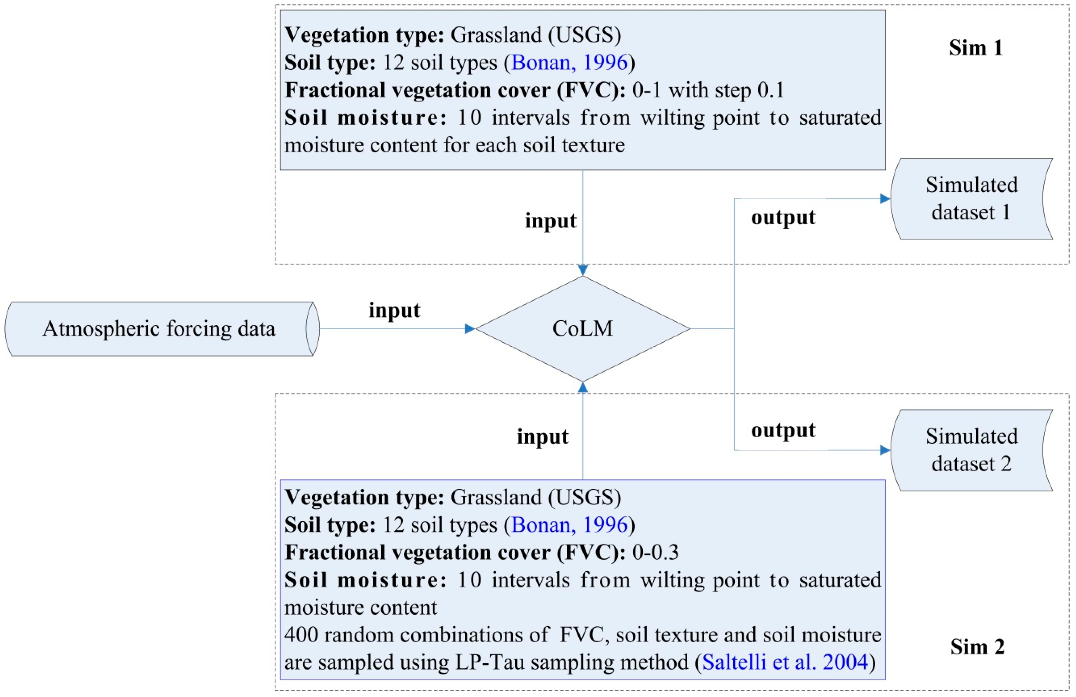
3.2. Land Surface Model Simulation

Because it is difficult to find a satellite pixel (approximately 10 km2) without the presence of vegetation on natural surfaces, except in desert regions, it is essential to investigate the feasibility of using the previous bare SSM retrieval model in vegetated conditions before applying the model to remotely sensed observations. To achieve this objective, a dataset, including SSM, as well as diurnal LST and NSSR cycles, with different underlying surfaces and atmospheric conditions is urgently needed for the development of the methodology. Because it is quite difficult to synchronously obtain these data with field measurements, a land surface model simulation is chosen as a feasible alternative to generate the dataset that is required for the development of a methodology for using the bare SSM retrieval model in vegetated conditions.
Figure 3. Scheme of the Common Land Model (CoLM) simulation.
Remotesensing 07 04112 g003
The Common Land Model (CoLM) is used to produce simulated data with different underlying surfaces and atmospheric conditions. In this study, hydraulic properties of 12 soil textures from the soil texture classification scheme of the Food and Agriculture Organization (FAO) are computed from Bonan (1996) [39]. Besides, the Grassland according to the United States Geological Survey (USGS) vegetation categories is set as the vegetation type in the CoLM simulation. In total, we perform two simulations in this study, namely sim1 and sim2, respectively. Figure 3 depicts the sim1 and sim2 in detail. For the sim1, the fractional vegetation cover (FVC) is set varying from 0 to 1 with a step of 0.1, and 10 intervals of initial soil moisture ranging from the minimum value (around the wilting point) to the maximum value (around the saturated moisture content) are used to represent different soil moisture status (Table 3). While for the sim2, the LP-Tau sampling method integrated in the Gaussian Emulation Machine-Sensitivity Analysis (GEM-SA) [40], is used to obtain totally 400 samples for a given atmospheric condition. For each sample, a unique combination of the soil texture, soil moisture and FVC is used to represent a possible underlying surface condition to initialize the CoLM. After the model initialization, the meteorological data of the selected cloud-free days at the three FLUXNET sites are utilized to drive the CoLM. The outputted diurnal cycles of LST and NSSR, as well as the daily average SSM, are collected to create the datasets and further used for the methodology development of the SSM retrieval model in vegetated conditions.
Table 3. Soil textures and surface soil moisture (SSM) ranges implemented in the Common Land Model (CoLM) simulation.
No.Sand (%)Silt (%)Clay (%)Soil TexturesRange of SSM (m3·m−3)
19253Sand0.010–0.339
282126Loamy Sand0.028–0.421
3583210Sandy Loam0.047–0.434
4177013Silt Loam0.084–0.476
510855Silt0.084–0.476
6433918Loam0.066–0.439
7581527Sandy Clay Loam0.067–0.404
8105634Silty Clay Loam0.120–0.464
9323434Clay Loam0.103–0.465
1052642Sandy Clay0.100–0.406
1164747Silty Clay0.126–0.468
12222058Clay0.138–0.468

4. Results and Discussion

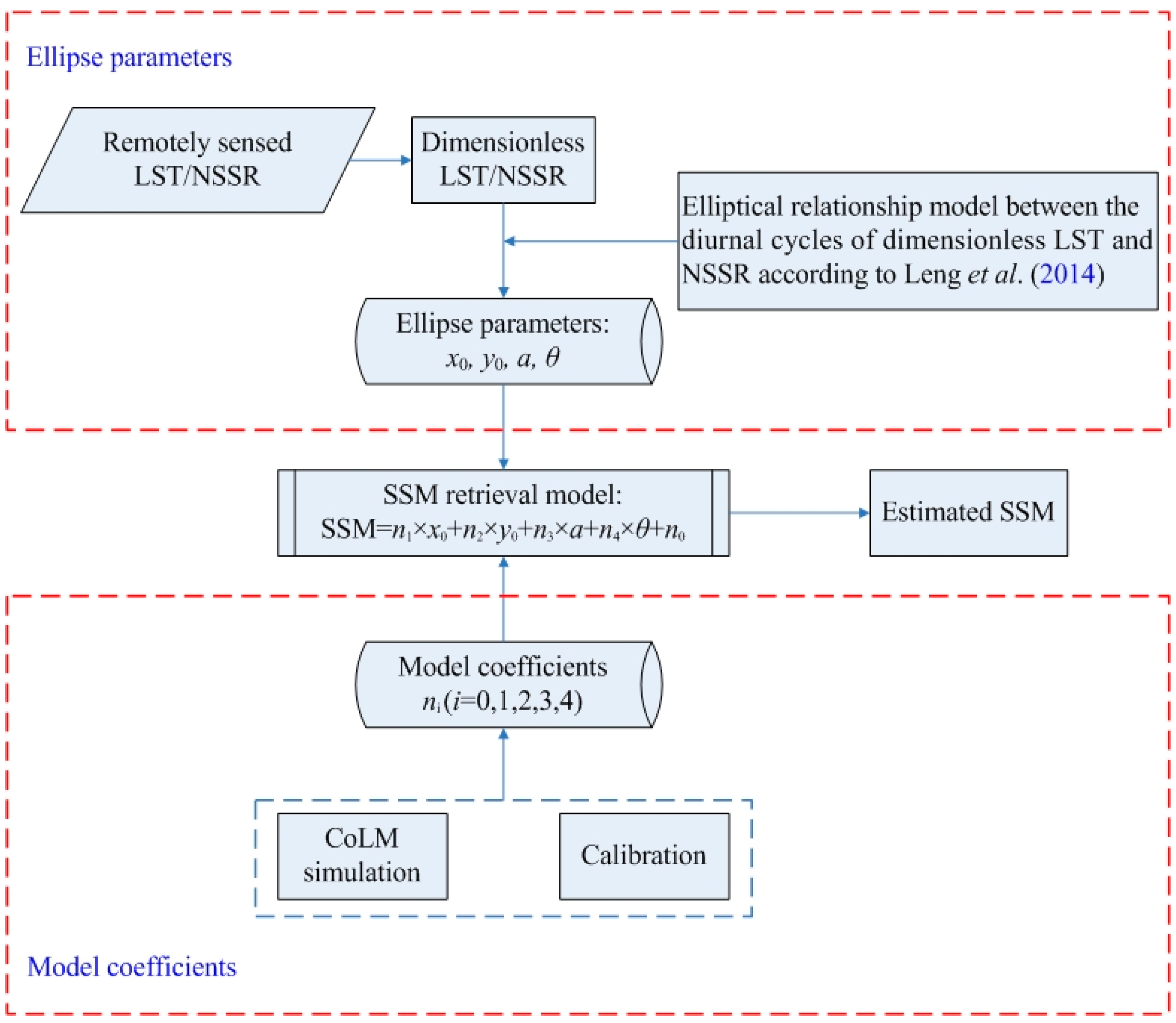
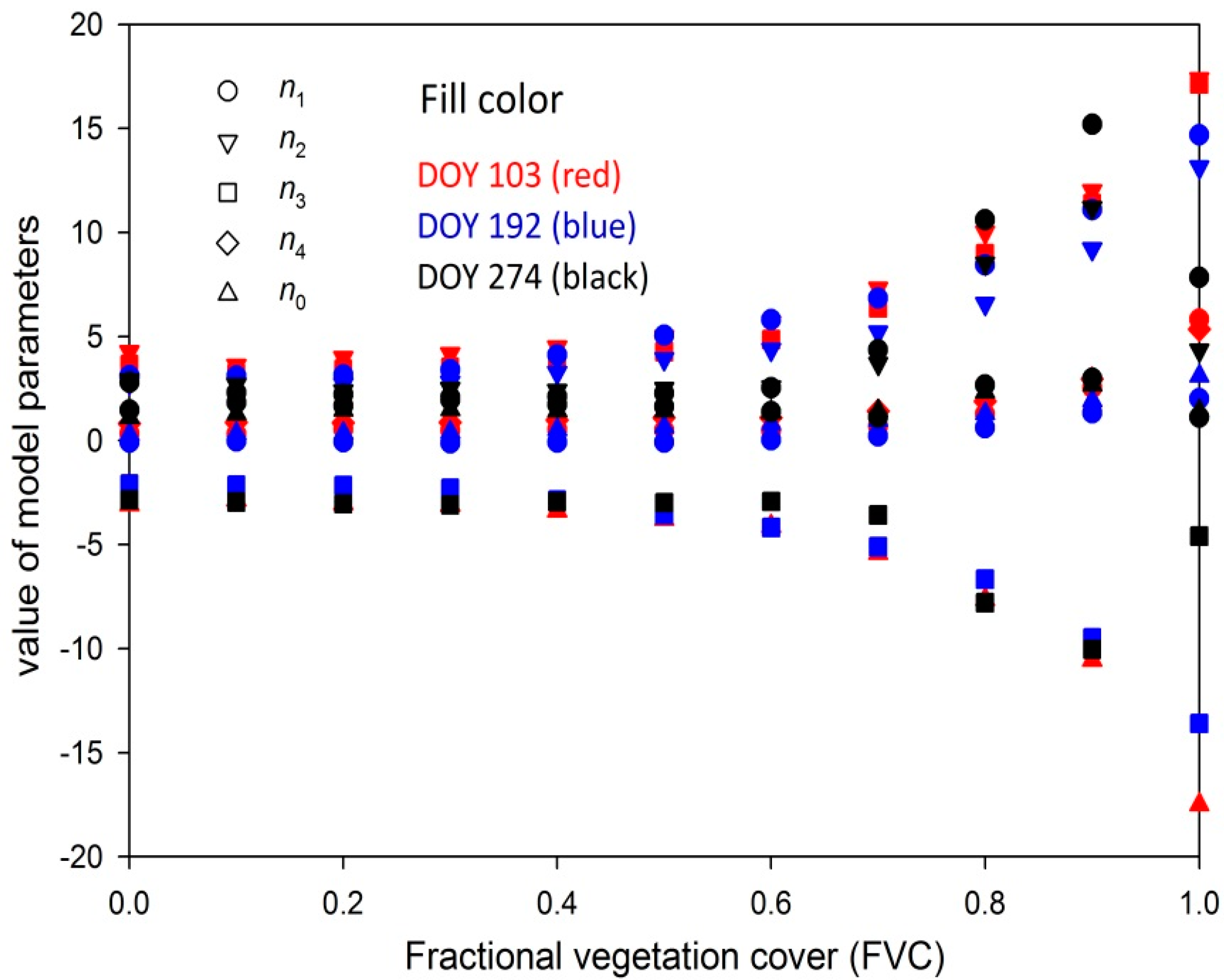
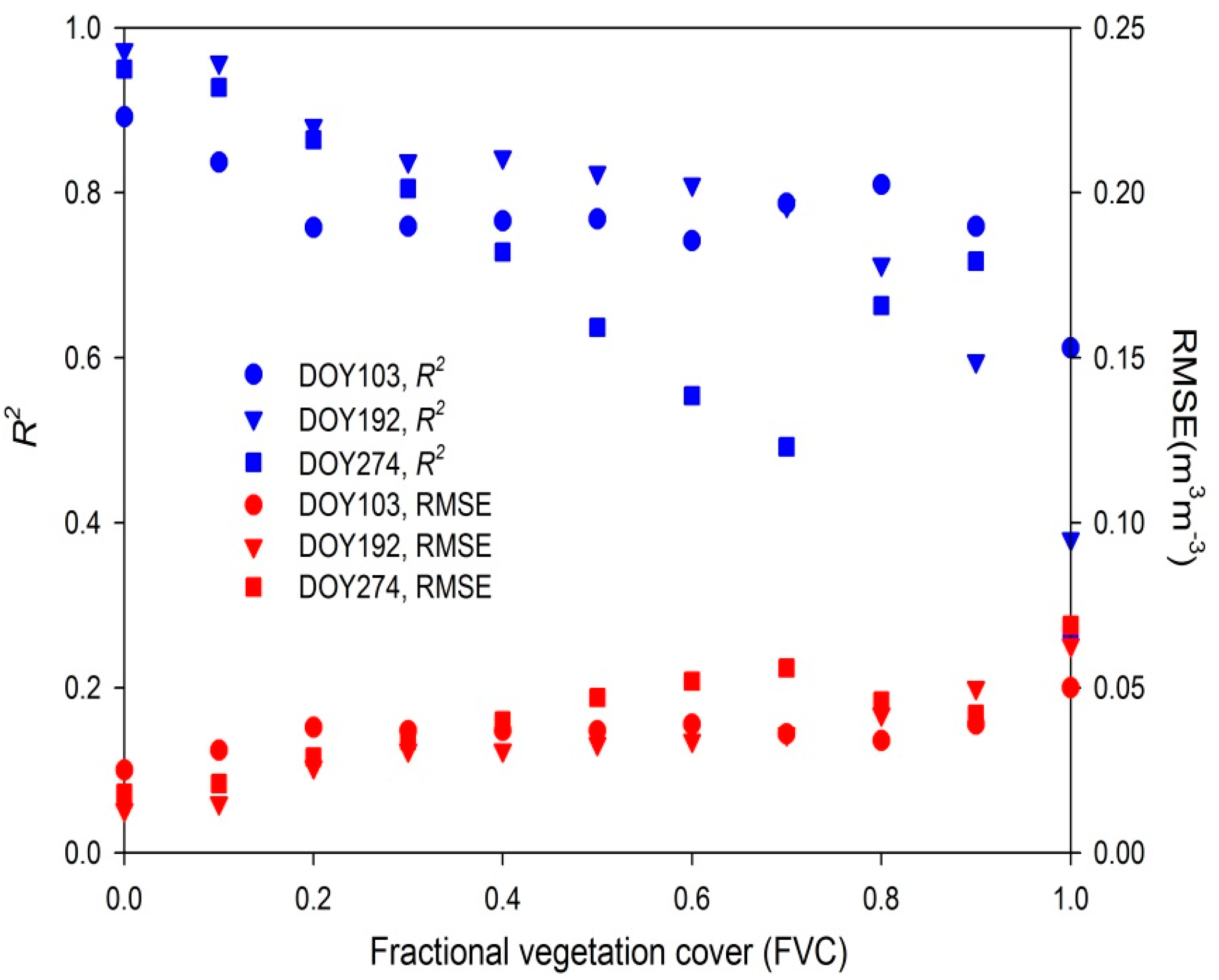
4.1. Effect of Vegetation on the Bare SSM Retrieval Model

Because the previous SSM retrieval model is originally developed for bare soils, simulated dataset from the sim1 are primarily used to investigate the effect of vegetation on the previous bare SSM retrieval using the model described in Equation (3). Analogous to previous study, simulated dataset1 on DOY 103, 192 and 274 in 2001 at the Bondville site is taken as an example. Figure 4 and Figure 5 show the results of SSM retrieval for different FVC using simulated data on these three cloud-free days. It is evident from Figure 4 that the model coefficients ni (i = 0, 1, 2, 3, 4) exhibit a stable and relatively regular variation when FVC varies from 0 to 0.7. When FVC is higher than 0.7, some of the model coefficients vary irregularly compared to the cases when FVC is lower than 0.7. In general, temperature and net shortwave radiation of the soil surface become extremely weak in the dense vegetation coverage (FVC > 0.7) conditions for remote sensing observations, and most of the signals are from the canopy. In that case, estimating SSM using such weak information from the optical/thermal measurements is most likely implying various uncertainties. For the accuracy of SSM retrieval, it exhibits overall a decrease with the increasing of FVC, which is probably due to the fact that signal of the soil suffers from a continuous attenuation with the increasing of vegetation coverage. In particular, it is clear from the Figure 5 that the SSM retrieval model maintains a relatively high accuracy (overall R2 around 0.8 and RMSE lower than 0.04m3m−3) in the low-cover vegetation conditions with FVC ranging from 0 to 0.3.
Figure 4. Variations of model parameters vs. fractional vegetation cover (FVC) with simulated data on DOY 103, 192 and 274 in 2001 at Bondville site.
Remotesensing 07 04112 g004
Figure 5. Variations of the accuracy of SSM retrieval vs. fractional vegetation cover (FVC) with simulated data on DOY 103, 192 and 274 in 2001 at Bondville site.
Remotesensing 07 04112 g005
In addition to the simulated results, ellipse parameters (x0, y0, a, b and θ) theoretically contain less information of soil with the increasing of FVC. Considering over-dense vegetation cover (FVC > 0.7), as canopy temperature takes a predominant role in the LST, signal from soil become negligible in comparison. Moreover, because vegetation has the ability to adjust the temperature to maintain vital activities through its strong physiological functions, canopy temperature will not exhibit drastic change with different soil moisture and soil texture conditions compared to bare soils, the ellipse parameters consequently vary in relatively narrow ranges. Figure 6 depicts the range of variation of the rotation angle (θ) vs. the FVC for soil Loam. In theory, a higher rotation angle (θ) responds to a higher SSM value for a given soil texture and atmospheric condition. As shown in Figure 6, it exhibits quite different ranges of rotation angle with different FVC for the same initial soil moisture conditions from the wilting point to the saturated moisture content. For dense vegetation cover, ellipse parameters generally vary in a relatively narrow range from both the simulated data and theoretical basis, which is unfavorable for the SSM estimation because small uncertainties of the ellipse parameters probably lead to a relatively significant error of SSM retrieval. It further indicates that dense vegetation cover is adverse to the estimation of SSM using the previously developed SSM retrieval model.
Nevertheless, considering the regular variation of model coefficients and accuracy when FVC is lower than 0.7, it remains possible to estimate SSM using a uniform expression in such a condition. In particular, results from the simulated data exhibit a relatively high accuracy when using the previous SSM retrieval model to estimate SSM in sparsely vegetated conditions (FVC lower than 0.3). Based on these, we mainly focus on the SSM retrieval in sparsely vegetated conditions in the present study.
Figure 6. Variation of the rotation angle (θ) vs. the fractional vegetation cover (FVC) for soil loam with the simulated data on DOY103, 192 and 274 in 2001 at Bondville site.
Remotesensing 07 04112 g006

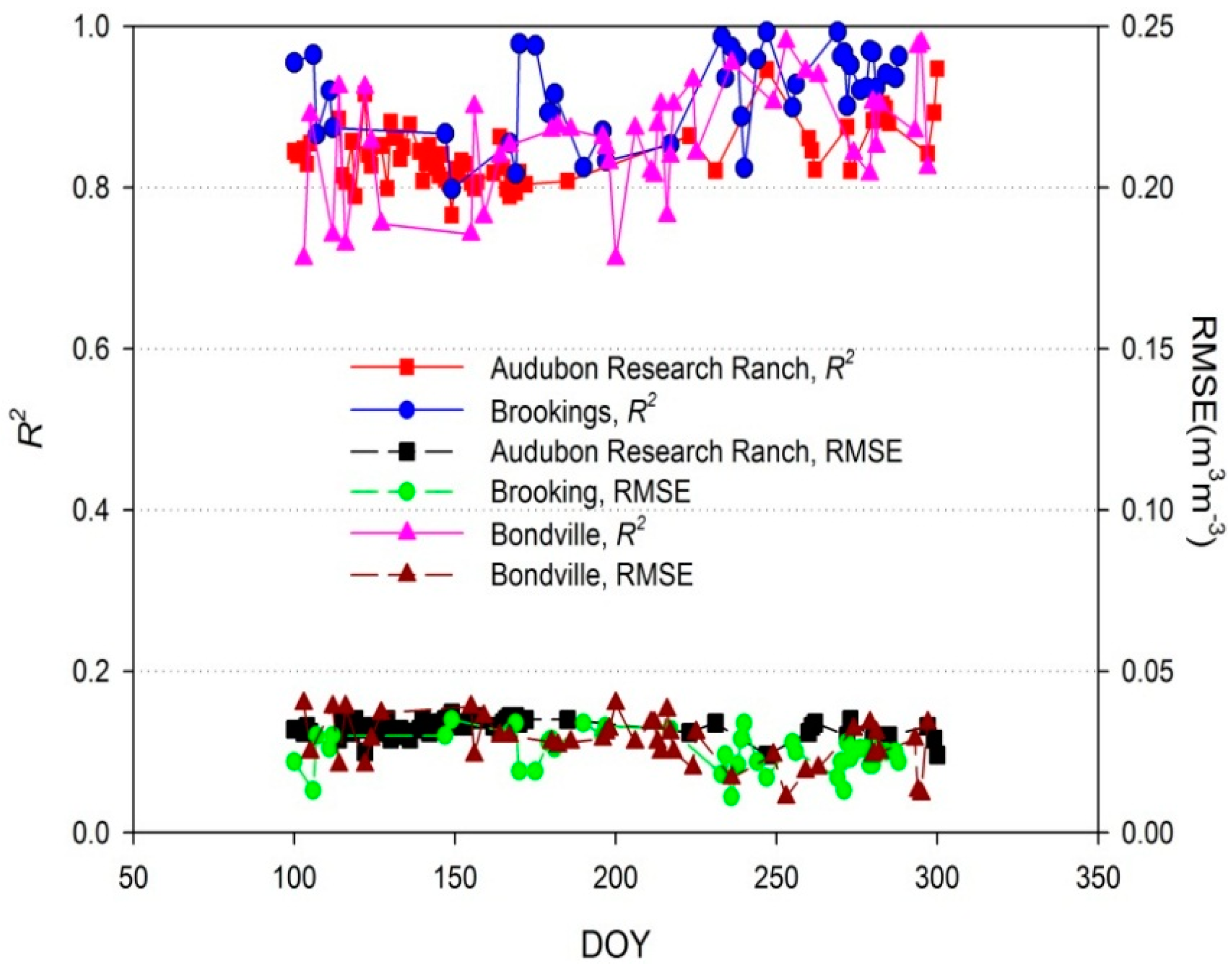
4.2. Feasibility of the SSM Retrieval Model in Sparsely Vegetated Conditions

Based on the simulated dataset, the feasibility of using the SSM retrieval model in sparsely vegetated conditions is further investigated. In general, this sparsely vegetated condition for SSM retrieval has been extensively studied in remote sensing technology, such as using the remotely sensed ATI or EF to estimate SSM. However, the present methods to retrieve SSM from the remotely sensed ATI or EF are indirect, and the empirical relationships between SSM and the remotely sensed ATI or EF are needed to obtain SSM at the regional scale. In this study, we mainly investigate the feasibility of using the previous bare SSM retrieval model to estimate SSM in sparsely vegetated conditions, which will be quite promising to estimate SSM directly from the remotely sensed ellipse parameters that derived from the diurnal LST and NSSR.
The simulated dataset2 on the eight cloud-free days at Bondville site in 2001 is used here as an example to address this issue. With the SSM retrieval model proposed in Equation (3), where the SSM is set as the dependent variable and the four ellipse parameters x0, y0, a and θ the independent variables, the five model coefficients ni (i = 0, 1, 2, 3, 4) are obtained through a least squares method. Table 4 shows the results of the five model coefficients ni (i = 0, 1, 2, 3, 4) and corresponding accuracy on these eight cloud-free days. It is evident that the previous bare SSM retrieval model exhibits generally high accuracy to estimate SSM in sparsely vegetated condition. The coefficient of determination (R2) ranges from 0.789 to 0.970, and the Root Mean Square Error (RMSE) varies from 0.012 to 0.033 m3·m−3 for the eight cloud-free days. Moreover, the mean R2 and RMSE for these eight cloud-free days are 0.876 and 0.025 m3·m−3, respectively, which indicates that the previous bare SSM retrieval model is feasible in sparsely vegetated conditions.
Table 4. Model coefficients and surface soil moisture (SSM) retrieval accuracy in sparsely vegetated conditions on the eight selected cloud-free days in the year 2001 at Bondville site.
DOYn1n2n3n4n0R2RMSE (m3·m−3)
1030.1823.6893.2780.768−2.7230.8550.027
128−0.4513.6923.0630.262−1.9100.7920.032
167−0.1883.5192.9330.218−1.9180.9570.015
192−0.1403.0832.7970.272−2.0260.9700.012
216−0.2583.1992.4950.384−1.9230.8070.032
2480.1833.5902.8340.793−2.5970.7890.033
2740.6673.0162.7110.864−2.3300.9170.021
2980.1134.9723.9820.422−2.2120.9250.020
Mean 0.8760.025
Because the results from Table 4 are merely based on the data simulated at the Bondville site, to determine the general SSM retrieval feasibility in sparsely vegetated conditions with different regions and climate patterns, further evaluation is conducted utilizing the simulated data on the other 151 cloud-free days at the Audubon Research Ranch, Brookings and Bondville sites. Results for all these 151 cloud-free days are presented in Figure 7. Although these three FLUXNET sites belong to different climate patterns, and the atmospheric conditions vary quite differently from these cloud-free days at the three sites, the accuracy of the SSM retrieval maintains a relative high level, with the R2 ranging from 0.712 to 0.993 and the RMSE from 0.011 to 0.040 m3·m−3. For the 151 days, the mean RMSE and R2 are approximately 0.028 m3·m−3 and 0.869, respectively. This result exhibits significant agreement between the estimated SSM and the simulated values, which further confirms that the use of the SSM retrieval model is feasible in sparsely vegetated condition. Note that for the simulated data on the 151 cloud-free days, only the meteorological data vary for each day, which lead to the variations of the five model coefficients ni (i = 0, 1, 2, 3, 4) and the corresponding accuracy of the SSM retrieval.
Figure 7. The coefficient of determination (R2) and Root Mean Square Error (RMSE) values of the surface soil moisture (SSM) retrieval in the sparsely vegetated conditions for the cloud-free days at the Audubon Research Ranch site (66 cloud-free days), Brookings site (41 cloud-free days) and Bondville site (44 cloud-free days).
Remotesensing 07 04112 g007

4.3. Determination of Model Coefficients from Satellite Observations and Ground SSM Measurements

The previous section indicates that the use of the SSM retrieval model is feasible in sparsely vegetated conditions with simulated data. As described earlier, the five model coefficients ni (i = 0, 1, 2, 3, 4) for each cloud-free day primarily depend on the atmospheric conditions, and they are essential for the application of the SSM retrieval model. In general, because the model coefficients depend on atmospheric conditions, they can be obtained by a land surface model simulation only if the meteorological data are available in the study area, as shown in previous sections. However, meteorological data probably does not always fulfill the requirements by a land surface model simulation. In theory, when the meteorological data are not available for the simulation to obtain the five model coefficients, ni (i = 0, 1, 2, 3, 4), the five model coefficients can also be acquired by at least five groups of synchronous observations (the ellipse parameters and the corresponding SSM) according to Equation (3). In this section, because the meteorological data collected at the REMEDHUS soil moisture network fail to meet the requirements to drive the CoLM, the SSM measurements from the REMEDHUS soil moisture network, together with the ellipse parameters (x0, y0, a and θ) derived from the MSG products, are explored to obtain the five model coefficients ni (i = 0, 1, 2, 3, 4) for each of the cloud-free days.
As mentioned in Table 2, the numbers of line and sample of the 19 soil moisture sites in the REMEDHUS soil moisture network are calculated based on the MSG data. Figure 8 depicts the 19 soil moisture sites and the FVC that is derived from the MSG FVC product based on the 11 × 8 MSG pixel rectangle area obtained on 15 July 2010. As illustrated by the figure, the 19 soil moisture measurement sites are uniformly distributed across the REMEDHUS region, where the FVC exhibits a relatively low values ranging from 0 to 0.30. Hence, the REMEDHUS soil moisture network region can be regarded as a sparsely vegetated area.
Figure 8. The fractional vegetation cover (FVC) values derived from the Meteosat Second Generation (MSG) FVC product of the REMEDHUS soil moisture network region on 15 July 2010.
Remotesensing 07 04112 g008
Previous studies have noted that the REMEDHUS region is relatively flat and features low heterogeneity, and the point-scale soil moisture data exhibit generally significant linear relationships with regional-scale soil moisture in this region [32]. Because no adequate MSG pixel-scale SSM data or other proxies are available at present, it is assumed that the SSM measured at each REMEDHUS site is capable of representing the SSM value of the corresponding MSG pixel. As illustrated by Figure 8, most of the soil moisture sites take one specific MSG pixel, and only L07 and M05 share a pixel, for which the average value of the two sites is used as the SSM. Therefore, a total of 18 SSM measurements, together with the corresponding ellipse parameters (x0, y0, a and θ) derived from the elliptical relationship between the diurnal cycles of MSG-derived LST and NSSR from 8:00 to 16:00 for each of the cloud-free days, are used to obtain an optimal solution for the five model ni (i = 0, 1, 2, 3, 4) according to Equation (3).
In the process of obtaining the five model coefficients, the SSM measurements that are significantly higher than the saturated soil moisture content have been discarded. A multiple linear regression with a 95% confidence level is further used to identify outliers in the regression and to obtain the five model coefficients ni (i = 0, 1, 2, 3, 4). Figure 9 depicts the sample size used in the process of obtaining the five model coefficients for each of the 59 cloud-free days. It is evident that except for a tiny handful of sites that with soil moisture measurements higher than saturated moisture content and the outliers identified by the regression with the 95% confidence level, in most of the 59 cloud-free days over 14 site SSM measurements (total is 18) have been used to calculate the five model coefficients ni (i = 0, 1, 2, 3, 4) in the aforementioned calibration method.
With the five model coefficients ni (i = 0, 1, 2, 3, 4) for each of the 59 cloud-free days in the REMEDHUS region, the SSM can finally be estimated with the SSM retrieval model. The comparison of the estimated SSM vs. the actual SSM for the 59 cloud-free days is shown in Figure 10. Compared with the accuracy of the SSM retrieval using simulated data (mean R2 = 0.869 and RMSE = 0.028 m3·m−3), the SSM estimation using the model coefficients derived from the actual data (MSG satellite products and REMEDHUS soil moisture measurements) exhibits a lower accuracy. Nevertheless, the results achieve a fairly accuracy (R2 = 0.552 with RMSE = 0.055 m3·m−3) for the 59 cloud-free days.
Figure 9. Sample size of the site SSM measurements involved in the process of calculating the five model coefficients ni (i = 0, 1, 2, 3, 4) for the selected cloud-free days in 2010 and 2011 at REMEDHUS soil moisture network.
Remotesensing 07 04112 g009
Figure 10. Comparison of the estimated SSM vs. the actual SSM on the 59 selected cloud-free days in the years 2010 and 2011. The model coefficients are obtained from the REMEDHUS soil moisture measurements and the Meteosat Second Generation (MSG) observations.
Remotesensing 07 04112 g010
Although the accuracy of the SSM retrieval using actual data is lower than that using the simulated data, mean RMSE of the 59 cloud-free days is generally acceptable (around the target accuracy of SMOS soil moisture products 0.04 m3·m−3), given that the simulated data primarily describe an ideal situation. The uncertainties in the SSM retrieval using the model coefficients derived from the actual data can be attributed to several sources of error. Because there are no better ways to obtain the MSG pixel SSM values with an acceptable accuracy at present, the primary error source is the assumption that the site SSM measurements represent the MSG pixel SSM values. Although the site measurements of SSM most likely have a certain degree of representativeness due to the underlying surface and a previous study [32], they are not the true pixel SSM values. A feasible method is suggested to implement more intensive SSM observations to produce better SSM value representativeness at the pixel-scale using field measurements. The second error source is most likely from the MSG products. According to the validation reports, the accuracy of the LST is generally lower than 2 K, and the monthly bias values for the DSSF are within ±5% in the majority of cases. Meanwhile, the absolute bias for the visible broadband albedo is approximately 1%. As the MSG products are used in this study to derive the ellipse parameters and subsequently to estimate SSM, the uncertainties of these MSG products may also lead to error in the SSM retrieval. Except for the two aforesaid error sources, the SSM retrieval model itself also has a certain error according to the simulated results in previous sections. Additionally, although a small number of measured SSM values with soil moisture content values that are significantly higher than saturation have been discarded, error may also exist in the other SSM measurements. This error may affect the model coefficients and subsequently influence the SSM retrieval.

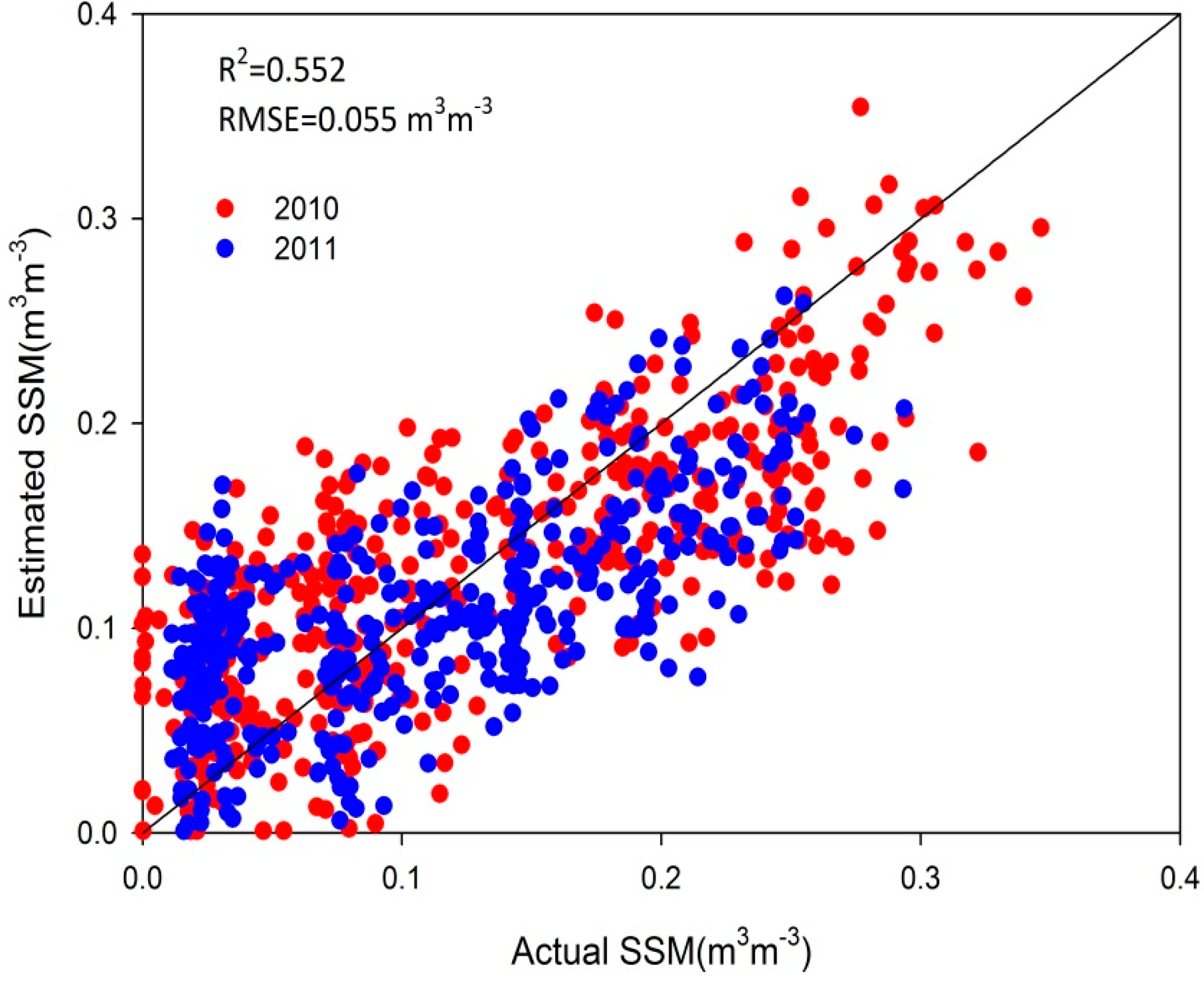
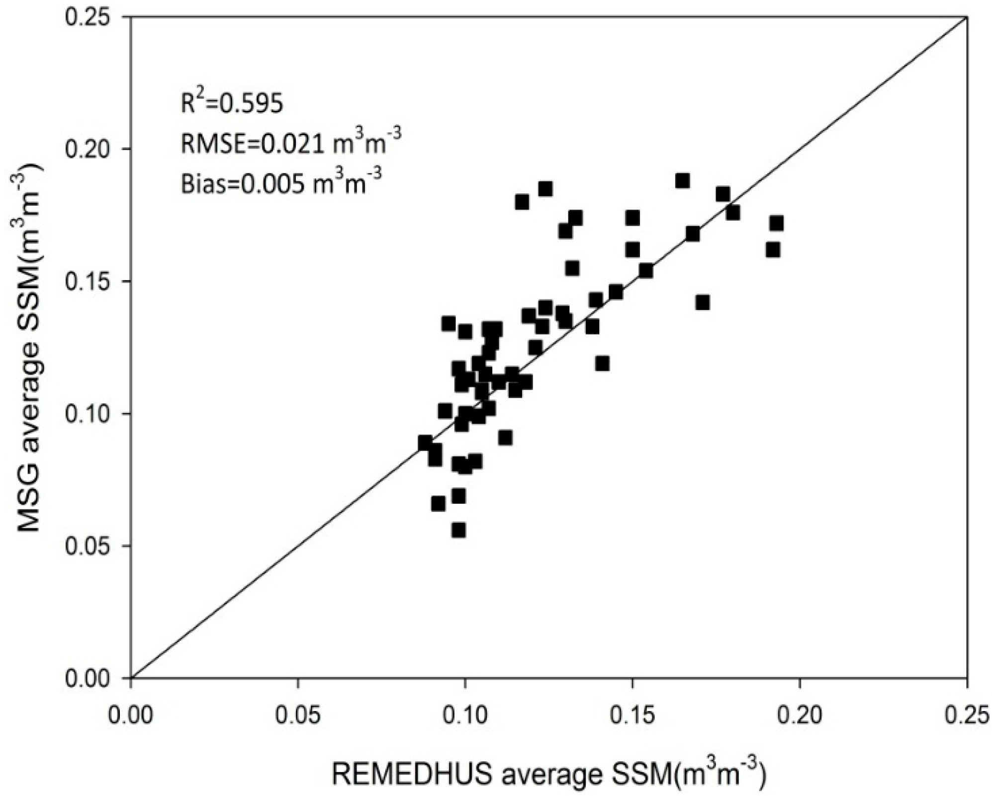
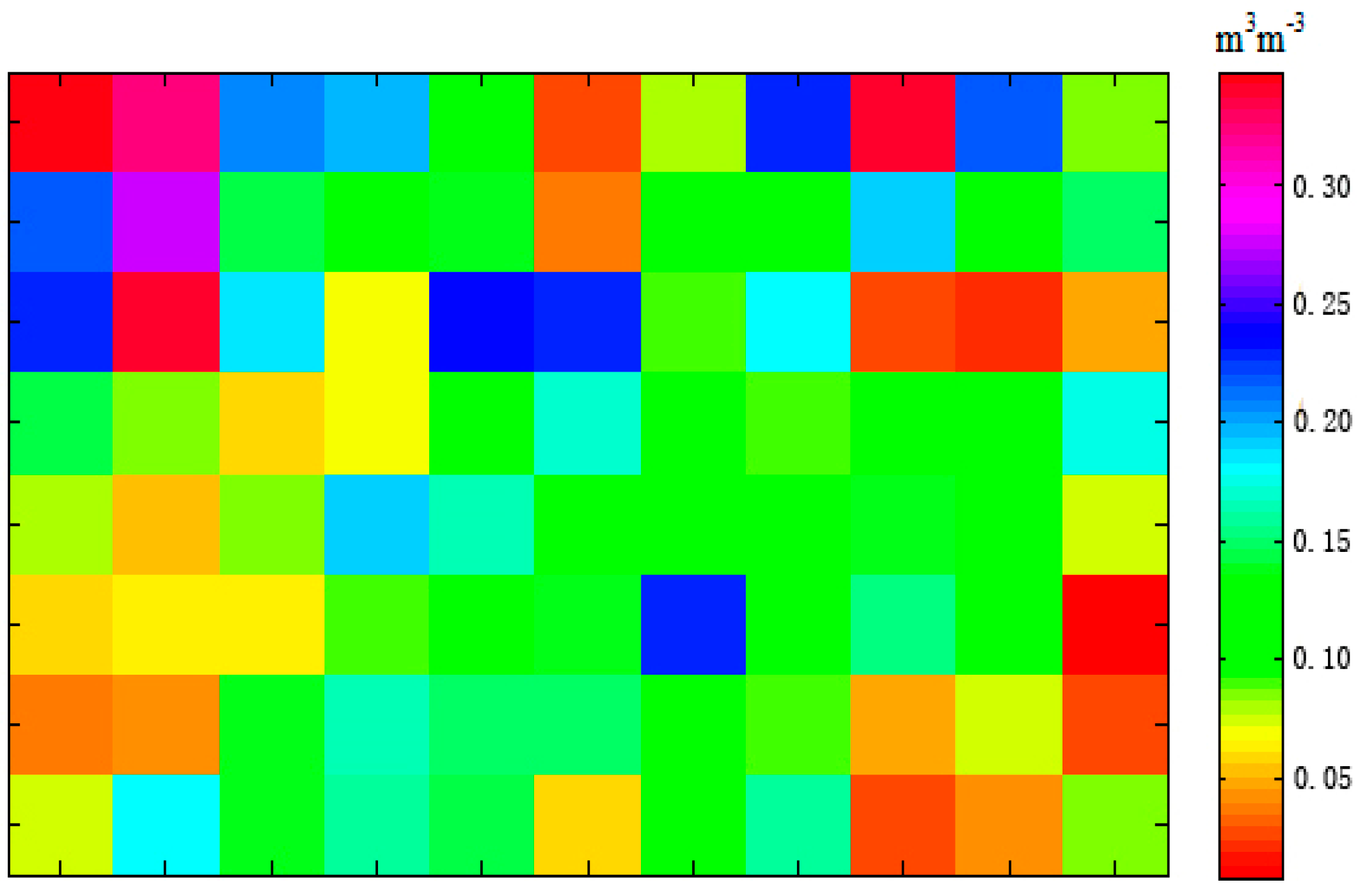
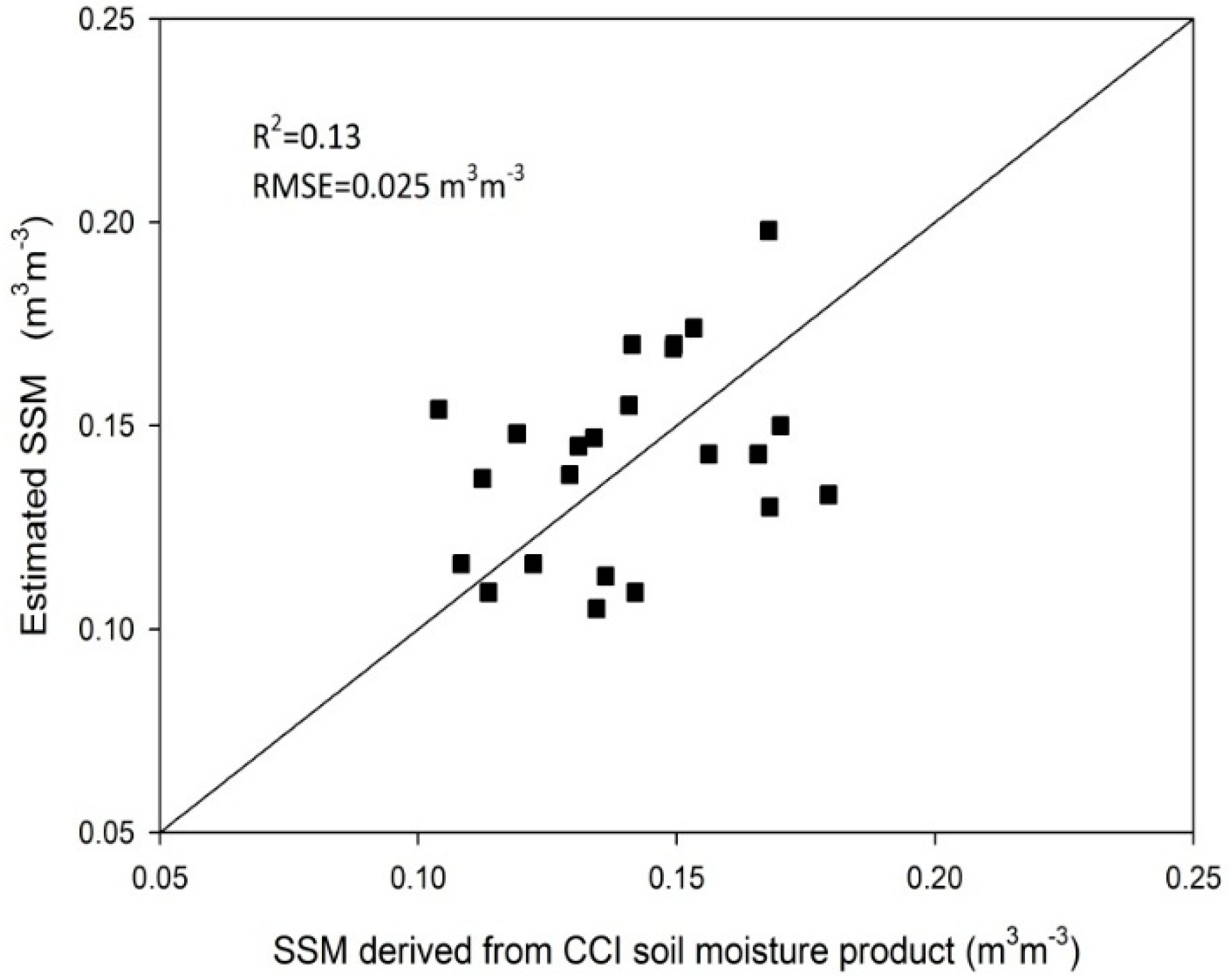
4.4. Surface Soil Moisture Retrieval and Preliminary Validation

As the REMEDHUS soil moisture network region in this study merely takes an 11 × 8 MSG pixel area (about 33 km × 24 km), atmospheric conditions in such a small region will not vary significantly for remote sensing. Consequently, the model coefficients ni (i = 0, 1, 2, 3, 4) determined from the synergistic use of the ten MSG observations and corresponding SSM measurements are theoretically applicable for the total 88 pixels within this region for each cloud-free day. Based on these, with the model coefficients obtained from the previous section and the ellipse parameters for each MSG pixel derived from the MSG observations (Table A1 shows an example of ellipse parameters on 15 July 2010), the quantitative SSM values with the MSG pixel-scale at the REMEDHUS soil moisture network region are finally estimated directly via the SSM retrieval model in Equation (3) for each of the cloud-free days. Figure 11 depicts the retrieved volumetric SSM content on 15 July 2010.
Because no adequate SSM estimates at the MSG pixel-scale or at higher spatial resolution are available at present, and downscaling methodologies for obtaining higher spatial resolution soil moisture data from the low spatial passive remote sensing soil moisture products still need to be improved [41], the retrieved volumetric SSM content cannot be validated directly. Nevertheless, we implement a preliminary validation to verify the results using SSM site measurements. Firstly, because the site SSM measurements are usually averaged to validate the SSM estimates at the pixel scale [31,34], we obtain an average SSM by taking the arithmetic mean of the site measurements in the REMEDHUS region for each cloud-free day, and these arithmetic mean values are regarded as REMEDHUS average SSM. Secondly, except for the ten MSG pixels that combined with SSM measurements to calculate the model coefficients, estimated SSM at the rest of the 11 × 8 MSG pixels are averaged to represent the retrieved average SSM of the REMEDHUS region. Because these rest pixels take an overwhelming majority of the whole 11 × 8 MSG pixels, their mean value is generally reasonable to represent the average SSM of the REMEDHUS region. In particular, using the rest of the pixel-scale SSM values rather than the whole 88 pixels for the validation can also avoid the repeated use of the ten SSM measurements in both model coefficients’ obtaining and SSM validation. Finally, the MSG average SSM values of the REMEDHUS region on the 59 cloud-free days are verified by the site average SSM values. Figure 12 depicts the result of this preliminary validation. It reveals a better consistency between the MSG average SSM values and the REMEDHUS site average SSM values, with a R2 of 0.595 and an RMSE of 0.021 m3·m−3. Additionally, a relatively small bias (0.005 m3·m−3) is found in the validation, which further indicates that the model coefficients ni (i = 0, 1, 2, 3, 4) determined from the synergistic use of the ten several MSG observations and corresponding SSM measurements are feasible to estimate SSM in the whole REMEDHUS region.
Figure 11. Retrieved volumetric SSM content (m3·m−3) using the Meteosat Second Generation (MSG) data in the REMEDHUS soil moisture network region on 15 July 2010.
Remotesensing 07 04112 g011
Figure 12. Comparison of the Meteosat Second Generation (MSG) pixels’ average SSM values vs. the soil moisture sites’ average surface soil moisture (SSM) values for the 59 selected cloud-free days in 2010 and 2011.
Remotesensing 07 04112 g012
In addition to this preliminary validation, products developed within the Soil Moisture CCI (Climate Change Initiative) project have also been used to validate the estimated results. In the CCI project, daily soil moisture product (layer depth of 0.5–2 cm) with a spatial resolution of 0.25° is provided from 1978 to 2010 [42]. In the present study, the estimated SSM with the MSG pixel scale are aggregated to the CCI spatial resolution in the REMEDHUS region for the selected cloud-free days in 2010 and subsequently to be verified using the available CCI soil moisture product. Figure 13 shows the comparison between the estimated SSM and the CCI soil moisture products; a R2 of 0.13 with an RMSE of 0.025 m3·m−3 is found between these two datasets.
Figure 13. Comparison of the estimated SSM and the CCI soil moisture product.
Remotesensing 07 04112 g013

4.5. Prospects of the Surface Soil Moisture Retrieval Model

The present study primarily investigates the possibility of using a previously developed bare SSM retrieval model in sparsely vegetated conditions. Results from the simulated data at three FLUXNET sites with different climate types exhibit a relatively stable and high accuracy on the SSM retrieval throughout growing seasons, which indicates that the SSM retrieval model is feasible. In particular, a preliminary validation from the REMEDHUS network with geostationary observations further implies an anticipated potential of applying the SSM retrieval model to the remotely sensed images to obtain SSM quantitatively. Nevertheless, several challenges remain to be properly addressed before the SSM retrieval model can be used for real satellite images to map and monitor time series SSM at the regional scale.
The first challenge is the determination of the five model coefficients ni (i = 0, 1, 2, 3, 4) at the regional scale. Although a relatively small bias is found in the preliminary validation in which the five model coefficients are calculated by the synergistic MSG observations and SSM measurements in the REMEDHUS region, it is quite difficult for real applications to obtain the model coefficients in this way regarding the sparse field SSM measurements with respect to a large and especially heterogeneous area. As we know, the five model coefficients depend only on the atmospheric conditions of each cloud-free day according to the results and analysis from the simulated data in the previous section, and they can be theoretically obtained by a land surface model (e.g., the CoLM) simulation with meteorological data collected in the study area. Hence, the quantity and distribution of the meteorological station at the regional scale is most likely to be a key point that will greatly affect the accuracy of SSM retrieval. In the ongoing work, considering the availability of meteorological data, we have been focusing on the parameterization of the five model coefficients ni (i = 0, 1, 2, 3, 4) using only meteorological elements themselves rather than appearing with data simulation by a land surface model (e.g., the CoLM) with strong physical basis. Moreover, we will also try in a future study to assess the feasibility of parameterizing the model coefficients using the publicly available weather forecast information. Only in that way can the SSM retrieval model be operational to map regional SSM using geostationary satellite images.
In addition to the model coefficients, acquisition of the ellipse parameters from the geostationary satellite observations is another challenge directly associated with the SSM estimates using the proposed SSM retrieval model. Because the ellipse parameters (x0, y0, a and θ) in the SSM retrieval model are calculated based on the elliptical relationship between diurnal cycles of LST and NSSR, it is evident that the accuracy of SSM retrieval is directly relying on the accuracy of geostationary satellite images derived-LST and NSSR. Namely, developing more feasible algorithms and reducing uncertainty in the LST and NSSR estimation from geostationary satellite data are effective ways to obtain SSM with better accuracy. Besides, because satellites always observe the Earth with a different time and angle for pixels within a certain study area at the regional scale, another possible approach to improve the accuracy of SSM retrieval using the proposed SSM retrieval model is through a time and angular normalization process to obtain LST and NSSR in a unified observation time and angle. Moreover, considering that the elliptical relationship is only valid for cloud-free days, this SSM retrieval model is most likely limited in the practical applications since the weather condition will not always satisfy the requirements by the SSM retrieval model. However, because the proposed SSM retrieval model uses the temporal rather than the instantaneous information from the LST and NSSR, and at least five synchronous LST and NSSR can form the elliptical relationship, a few images during a day may not affect the application of the SSM retrieval model. Nevertheless, more effort should be made on the quantitative retrieval of LST and NSSR, and especially the obtaining of the diurnal curves of these two land surface variables not only for cloud-free days, to ensure the feasibility of using the proposed SSM retrieval model with geostationary satellite observations. With all these efforts, the SSM retrieval model can be really operational for long-term mapping and monitoring of SSM time series.
Finally, we would like to emphasize that the SSM retrieval model proposed in this study is quite different from the previous optical/thermal remote sensing methods to estimate SSM. In the present study, the five model coefficients ni (i = 0, 1, 2, 3, 4) are not the empirical coefficients linking the soil moisture and remotely sensed land surface variables (such as the coefficients in the ATI-SSM or EF-SSM empirical relationships). In theory, the five model coefficients ni (i = 0, 1, 2, 3, 4) depend only on the atmospheric conditions of each cloud-free day, and they can be obtained from a simulation by a land surface model (e.g., the CoLM) with strong physical basis as described in previous sections. Namely, in theory, ground SSM measurements are not required in the proposed SSM retrieval model to map a regional SSM. However, the traditional ATI-SSM or EF-SSM relationships usually need SSM measurements (either ground or satellite) to obtain the empirical coefficients. Specifically, these empirical relationships are not independent of soil texture. For the proposed SSM retrieval model, it is capable of estimating quantitative volumetric soil moisture content directly using geostationary satellite derived-LST and NSSR with the model coefficients obtained from a land surface model simulation for which only meteorological data are required.

5. Conclusions

In this study, we have primarily pursued the feasibility of a newly developed bare SSM retrieval model in vegetated conditions. Based on the SSM retrieval model for bare soils, simulated data were first used to evaluate the capability of the model in vegetated conditions. It was found that using the bare SSM retrieval model to estimate SSM is feasible in low-cover vegetation area, with FVC ranging from 0 to 0.3. The results of the simulated data from the CoLM have demonstrated that the estimated SSM is significant and linearly correlated with the simulated values. A mean RMSE of 0.028 m3·m−3 with a R2 of 0.869 were found between the estimated SSM values and the simulated values for the 151 cloud-free days at Audubon Research Ranch, Brookings sites and Bondville site. In addition to the simulated data, a preliminary validation of the SSM retrieval model using geostationary satellite data from the MSG were also presented. In particular, the obtaining of the five model coefficients ni (i = 0, 1, 2, 3, 4) from the combined use of the REMEDHUS soil moisture measurements and the MSG observations was explored in detail. This investigation indicated a feasible way to obtain the model coefficients in cases where the meteorological data are not available to drive the CoLM to acquire the model coefficients. Compared with the SSM retrieval using model coefficients derived from the land surface model simulation, the accuracy was lower when using model coefficients obtained from actual data. Nevertheless, the results from the 59 cloud-free days revealed an acceptable accuracy with a R2 of 0.552 and an RMSE of 0.055 m3·m−3. Additionally, some of the possible error sources were analyzed, and a number of recommendations were proposed to improve the accuracy of the SSM retrieval. Finally, the average SSM of the 11 × 8 MSG pixel rectangular area of the REMEDHUS soil moisture network region was preliminarily verified using the average SSM data from the site measurements for the SSM in this region. A R2 of 0.595 and an RMSE of 0.021 m3·m−3 were found. A relatively small bias of 0.005 m3·m−3 indicated that using the model coefficients derived from the actual data was feasible for the SSM retrieval in this region.
In summary, the use of the SSM retrieval model has been proven to be feasible in sparsely vegetated conditions with both simulated data and remotely sensed observations. In particular, the study has presented two methods to obtain the five model coefficients of the SSM retrieval model. One is through the simulation of a land surface model using meteorological data; the other is through the combined use of several field-based SSM measurements and geostationary observations when meteorological data are not available. Compared with the previous optical/thermal remote sensing to estimate SSM, because the present SSM retrieval model is capable of obtaining SSM directly from the remotely sensed ellipse parameters, and ground SSM measurements are not necessary in the SSM retrieval model, no empirical relationships are needed to link the measured SSM and the remotely sensed land surface parameters, such as the TVDI-SSM relationships and ATI-SSM relationships. Moreover, the model coefficients in the present SSM retrieval model are quite different from the empirical coefficients in the previous optical/thermal remote sensing for SSM retrieval. In the proposed SSM retrieval model, the model coefficients are theoretically dependent only on the atmospheric conditions of each cloud-free day, and they can be obtained from a simulation by a land surface model that with strong physical basis only if the meteorological data are available.
Although some issues with respect to making the SSM retrieval model more operational remain to be appropriately addressed, the model shows significant potential to estimate regional SSM using geostationary satellite data. For future development, we will attempt to apply and validate the SSM retrieval model with denser ground measurements and other remotely sensed observations, such as the FY data from China and the GOES data from the USA. In particular, the feasibility of the SSM retrieval model in densely vegetated conditions should be investigated in more depth in ongoing work.

Acknowledgments

The authors thank the International Soil Moisture Network (ISMN) for providing the soil moisture measurements data and FLUXNET for providing the meteorological data. We also thank the LSA-SAF for supplying the MSG products. Many thanks also to José Martínez-Fernández, University of Salamanca, Spain, for his enthusiastic help and useful data. The work described in this publication has been supported by the National Nature Science Foundation of China under grant No. 41271379, the Chinese Academy of Sciences (CAS) Key Research Program “Hydrological Impacts from Degrading Permafrost in the Sources Area of the Yellow River” under grant No. KZZD-EW-13, and the CAS Action-Plan for West Development under grant No. KZCX2-XB3-15. Pei Leng was financially supported by the China Scholarship Council (CSC) for his stay at the ICube laboratory, University of Strasbourg, France.

Author Contributions

Pei Leng conceived and designed the experiments with advice of Xiaoning Song and Zhao-Liang Li. Pei Leng performed the acquisition, analysis and interpretation of the data. Yawei Wang and Ruixin Wang performed the modeling. All authors discussed the basic structure of the manuscript, and Pei Leng finished the first draft. Xiaoning Song and Zhao-Liang Li reviewed and edited the draft. All authors read and approved the submitted manuscript, agreed to be listed and accepted the version for publication.

Conflicts of Interest

The authors declare no conflict of interest.

Appendix

Table A1. Ellipse parameters (x0, y0, a, b and θ) derived from MSG images at REMEDHUS soil moisture network region (11 × 8 MSG pixels) on 15 July 2010. Line and sample describe each pixel in the European portion of the Meteosat Second Generation (MSG) data.
LineSamplex0y0abθ
4741600.50720.28350.49290.09980.8997
4741610.50120.29480.47810.09490.9201
4741620.56430.34680.39880.08150.8571
4741630.51210.26930.49190.08910.8519
4741640.56650.32510.40300.08820.8672
4741650.56920.35430.34860.09200.9170
4741660.53400.34690.36390.08370.9885
4741670.58000.40840.32970.07750.9038
4741680.52370.32740.44550.08860.9003
4741690.54050.34800.39310.08610.9328
4741700.59510.40160.30400.07890.9138
4751600.61170.42030.32530.08190.8063
4751610.57020.37490.37960.08420.8654
4751620.55150.31460.43270.08020.8227
4751630.61990.38970.33180.07840.8043
4751640.48970.22750.53370.09590.8413
4751650.55340.30600.41670.09390.8504
4751660.58350.34570.36750.08590.8991
4751670.61620.41060.30410.08230.8676
4751680.53460.29850.43710.09280.9232
4751690.58020.34630.37090.08050.8844
4751700.55070.29110.44060.08690.8766
4761600.61210.38250.35750.07770.8126
4761610.42510.16740.64840.08970.8404
4761620.54040.28380.47960.07950.7862
4761630.59390.34850.38070.08050.7794
4761640.42970.16180.64550.09420.8003
4761650.35630.04540.77260.10430.8423
4761660.62930.38020.33740.07500.7847
4761670.52400.26850.48970.08850.8293
4761680.57730.34240.37480.07770.8350
4761690.53750.29060.43350.07990.8601
4761700.61280.37680.32680.07910.8487
4771600.54850.29960.44470.08330.8317
4771610.57910.34100.38850.07580.8155
4771620.59270.34580.37700.07560.8020
4771630.61100.35780.35730.07940.8083
4771640.61240.36620.35460.08150.8050
4771650.57370.30600.43330.08320.8164
4771660.60540.33710.38050.07950.8271
4771670.61950.37360.34390.07300.7998
4771680.55700.29950.42960.08300.8455
4771690.54450.28270.45410.08240.8534
4771700.44210.15820.61870.09490.8616
4781600.54870.30560.42280.08090.8623
4781610.55340.31600.41340.07950.8372
4781620.46540.21330.55500.08620.8256
4781630.54730.27790.46620.08610.8482
4781640.56590.30480.42910.08810.8500
4781650.58280.32970.40200.08710.8203
4781660.62950.35980.35120.08010.8093
4781670.62030.34700.37090.07830.7995
4781680.60820.33830.38810.08050.7962
4781690.61960.36350.35850.07800.7887
4781700.58660.34110.38630.07810.8020
4791600.52920.29730.42660.08390.8688
4791610.57160.33730.38370.08050.8509
4791620.60020.37110.34910.07640.8130
4791630.56470.31990.40990.08550.8350
4791640.52670.26060.48190.08730.8428
4791650.57000.30150.43450.08470.8179
4791660.50260.22120.55730.08660.7930
4791670.59430.31590.41580.08210.7677
4791680.50600.23480.52960.08810.8072
4791690.56040.30840.42990.07930.8281
4791700.60330.36630.33840.07710.8344
4801600.59510.37410.32570.08210.8933
4801610.60160.39230.31850.07430.8477
4801620.58370.35410.37530.07370.8456
4801630.50810.24200.51200.08890.8561
4801640.60170.34410.38710.07870.8016
4801650.59170.31800.41940.08120.7794
4801660.61680.35010.37730.07950.7690
4801670.56290.29260.44100.08190.8079
4801680.61960.36320.33290.07750.8190
4801690.59740.34700.36780.07650.8335
4801700.58050.34420.37190.07800.8359
4811600.59680.38440.32530.07790.8775
4811610.52510.30240.44720.07880.8822
4811620.55600.32790.41560.07760.8322
4811630.55970.31720.43370.07630.8005
4811640.54550.29720.45960.07760.7863
4811650.64920.39120.31750.07650.7645
4811660.61190.35390.37050.07580.7879
4811670.50240.22770.53390.08780.8264
4811680.58260.32120.39550.07540.8139
4811690.63960.39840.30490.06770.7613
4811700.61070.37660.34850.07410.7877

References

  1. Eltahir, E. A soil moisture-rainfall feedback mechanism, 1. Theory and observations. Water Resour. Res. 1998, 34, 765–776. [Google Scholar] [CrossRef]
  2. Entekhabi, D.; Rodriquez-Iturbe, I. Analytical framework for the characterization of the space-time variability of soil moisture. Adv. Water Resour. 1994, 17, 35–45. [Google Scholar] [CrossRef]
  3. Mintz, Y.; Serafini, Y. A global monthly climatology of soil moisture and water balance. Clim. Dyn. 1992, 8, 13–27. [Google Scholar] [CrossRef]
  4. Gokmen, M.; Vekerdy, Z.; Verhoef, A.; Verhoef, W.; Batelaan, O.; van der Tol, C. Integration of soil moisture in SEBS for improving evapotranspiration estimation under water stress conditions. Remote Sens. Environ. 2012, 121, 261–274. [Google Scholar] [CrossRef]
  5. Seneviratne, S.; Corti, T.; Davin, E.; Hirschi, M.; Jaeger, E.; Lehner, I.; Orlowsky, B.; Teuling, A. Investigating soil moisture-climate interactions in changing climate: A Review. Earth-Sci. Rev. 2010, 99, 125–161. [Google Scholar] [CrossRef]
  6. Szép, I.; Mika, J.; Dunkel, Z. Palmer drought severity index as soil moisture indicator: Physical interpretation, statistical behaviour and relation to global climate. Phys. Chem. Earth. 2005, 30, 231–243. [Google Scholar] [CrossRef]
  7. Krishnan, P.; Black, A.; Grant, J.; Barr, G.; Hogg, H.; Jassal, S.; Morgenstern, K. Impact of changing soil moisture distribution on net ecosystem productivity of boreal aspen forest during and following drought. Agric. For. Meteorol. 2006, 139, 208–223. [Google Scholar] [CrossRef]
  8. Qian, B.; Jong, R.; Gameda, S. Multivariate analysis of water-related agroclimatic factors limiting spring wheat yields on the Canadian prairies. Eur. J. Agron. 2009, 30, 140–150. [Google Scholar] [CrossRef]
  9. Hupet, F.; Vanclooster, M. Intraseasonal dynamics of soil moisture variability within a small agricultural maize cropped field. J. Hydrol. 2002, 261, 86–101. [Google Scholar] [CrossRef]
  10. Champagne, C.; Berg, A.A.; McNairn, H.; Drewitt, G.; Huffman, T. Evaluation of soil moisture extremes for agricultural productivity in the Canadian prairies. Agric. For. Meteorol. 2012, 165, 1–11. [Google Scholar] [CrossRef]
  11. Porporato, A.; D’Odorico, P.; Laio, F.; Rodriquez-Iturbe, I. Hydrologic controls on soil carbon and nitrogen cycles. I. Modeling scheme. Adv. Water Resour. 2003, 26, 45–58. [Google Scholar] [CrossRef]
  12. Yurova, A.Y.; Lankreijer, H. Carbon storage in the organic layers of boreal forest soils under various moisture conditions: A model study for northern Sweden sites. Ecol. Model. 2007, 204, 475–484. [Google Scholar] [CrossRef]
  13. Njoku, E.G.; Jackson, T.J.; Lakshmi, V.; Chan, T.K.; Nghiem, S.V. Soil moisture retrieval from AMSR-E. IEEE Trans. Geosci. Remote Sens. 2003, 41, 215–229. [Google Scholar] [CrossRef]
  14. Kerr, Y.H.; Waldteufel, P.; Wigneron, J.P.; Martinuzzi, J.; Font, J.; Berger, M. Soil moisture retrieval from space: The Soil Moisture and Ocean Salinity (SMOS) mission. IEEE Trans. Geosci. Remote Sens. 2001, 39, 1729–1735. [Google Scholar] [CrossRef]
  15. Entekhabi, D.; Njoku, E.G.; O’Neill, P.E.; Kellogg, K.H.; Crow, W.T.; Edelstein, W.N.; Entin, J.K.; Goodman, S.D.; Jackson, T.J.; Johnson, J.; et al. The Soil Moisture Active Passive (SMAP) mission. Proc. IEEE 2010, 98, 704–716. [Google Scholar] [CrossRef]
  16. Njoku, E.G.; Entekhabi, D. Passive microwave remote sensing of soil moisture. J. Hydrol. 1996, 184, 101–129. [Google Scholar] [CrossRef]
  17. Wigneron, J.P.; Calvetb, J.C.; Pellarinb, T.; Van de Griendc, A.A.; Bergerd, M.; Ferrazzolie, P. Retrieving near-surface soil moisture from microwave radiometric observations: Current status and future plans. Remote Sens. Environ. 2003, 85, 489–506. [Google Scholar] [CrossRef]
  18. Carlson, T. An overview of the “Triangle Method” for estimating surface evapotranspiration and soil moisture from satellite imagery. Sensors 2007, 7, 1612–1629. [Google Scholar] [CrossRef]
  19. Wang, L.; Qu, J. Satellite remote sensing applications for surface soil moisture monitoring: A review. Front. Earth Sci. 2009, 3, 237–247. [Google Scholar] [CrossRef]
  20. Petropoulos, G.; Carlson, T.; Wooster, M.J.; Islam, S. A review of Ts/VI remote sensing based methods for the retrieval of land surface energy fluxes and soil surface moisture. Prog. Phys. Geogr. 2009, 33, 224–250. [Google Scholar] [CrossRef]
  21. Li, Z.-L.; Tang, R.L.; Wan, Z.; Bi, Y.; Zhou, C.; Tang, B.H.; Yan, G.; Zhang, X. A review of current methodologies for regional evapotranspiration estimation from remotely sensed data. Sensors 2009, 9, 3801–3853. [Google Scholar] [CrossRef] [PubMed]
  22. Li, Z.-L.; Tang, B.H.; Wu, H.; Ren, H.; Yan, G.; Wan, Z. Satellite-derived land surface temperature: Current status and perspectives. Remote Sens. Environ. 2013, 131, 14–37. [Google Scholar] [CrossRef]
  23. Li, Z.-L.; Wu, H.; Wang, N.; Qiu, S.; Sobrino, J.A.; Wan, Z.M.; Tang, B.H.; Yan, G.J. Land surface emissivity retrieval from satellite data. Int. J. Remote Sens. 2013, 34, 3084–3127. [Google Scholar] [CrossRef]
  24. Price, J.C. The potential of remotely sensed thermal infrared data to infer surface soil moisture and evaporation. Water Resour. Res. 1980, 16, 787–795. [Google Scholar] [CrossRef]
  25. Verstraeten, W.; Veroustraete, F.; Sande, C.; Grootaers, I.; Feyen, J. Soil moisture retrieval using thermal inertia, determined with visible and thermal spaceborne data, validated for European forests. Remote Sens. Environ. 2006, 101, 299–314. [Google Scholar] [CrossRef]
  26. Minacapilli, M.; Iovino, M.; Blanda, F. High resolution remote estimation of soil surface water content by a thermal inertia approach. J. Hydrol. 2009, 379, 229–238. [Google Scholar] [CrossRef]
  27. Davies, J.; Allen, C. Equilibrium, potential and actual evaporation from cropped surfaces in southern Ontario. J. Appl. Meteorol. 1973, 12, 649–657. [Google Scholar] [CrossRef]
  28. Sandholt, I.; Rasmussen, K.; Andersen, J. A simple interpretation of the surface temperature/vegetation index space for assessment of surface moisture status. Remote Sens. Environ. 2002, 79, 213–224. [Google Scholar] [CrossRef]
  29. Leng, P.; Song, X.; Li, Z.-L.; Ma, J.; Zhou, F.; Li, S. Bare surface soil moisture retrieval from the synergistic use of optical and thermal infrared data. Int. J. Remote Sens. 2014, 35, 988–1003. [Google Scholar] [CrossRef]
  30. Leng, P.; Song, X.; Li, Z.-L.; Wang, Y. Evaluation of the effects of soil layer classification in the common land model on modeled surface variables and the associated land surface soil moisture retrieval model. Remote Sens. 2013, 5, 5514–5529. [Google Scholar] [CrossRef]
  31. Ceballos, A.; Scipal, K.; Wagner, W.; Martínez-Fernández, J. Validation of ERS scatterometer-derived soil moisture data in the central part of the Duero basin, Spain. Hydrol. Process. 2005, 19, 1549–1566. [Google Scholar] [CrossRef]
  32. Wanger, W.; Naeimi, V.; Scipal, K.; de Jeu, R.; Martínez-Fernández, J. Soil moisture from operational meteorological satellites. Hydrogeol. J. 2007, 15, 121–131. [Google Scholar] [CrossRef]
  33. Wanger, W.; Pathe, C.; Doubkova, M.; Sabel, D.; Bartsch, A.; Hasenauer, S.; Blöschl, G.; Scipal, K.; Martínez-Fernández, J.; Löw, A. Temporal stability of soil moisture and radar backscatter observed by the Advanced Synthetic Aperture Radar (ASAR). Sensors 2008, 8, 1174–1197. [Google Scholar]
  34. Sánchez, N.; Martínez-Fernández, J.; Scaini, A.; Pérez-Gutiérrez, C. Validation of the SMOS L2 soil moisture data in the REMEDHUS network (Spain). IEEE Trans. Geosci. Remote Sens. 2012, 50, 1602–1611. [Google Scholar] [CrossRef]
  35. International Soil Moisture Network. Available online: http://ismn.geo.tuwien.ac.at/ (accessed on 10 November 2014).
  36. Sánchez, N.; Martínez-Fernández, J.; Calera, A.; Torres, E.; Pérez-Gutiérrez, C. Combining remote sensing and in situ soil moisture data for the application and validation of a distributed water balance model (HIDROMORE). Agric. Water Manag. 2010, 98, 69–78. [Google Scholar] [CrossRef]
  37. Schmetz, J.; Pili, P.; Tjemkes, S.; Just, D.; Kerkmann, J.; Rota, S.; Ratier, A. An introduction to Meteosat Second Generation (MSG). Bull. Amer. Meteor. Soc. 2002, 83, 977–992. [Google Scholar] [CrossRef]
  38. Land Surface Analysis Satellite Applications Facility (LSA-SAF). Available online: http://landsaf.meteo.pt/ (accessed on 10 November 2014).
  39. Bonan, G.B. A Land Surface Model (LSM Version 1.0) for Ecological, Hydrological, and Atmospheric Studies: Technical Description and User’s Guide; NCAR Technical NoteNCAR/TN-417+STR; National Center for Atmospheric Research: Boulder, CO, USA, 1996; p. 150. [Google Scholar]
  40. The GEM Software Project. Available online: http://www.tonyohagan.co.uk/academic/GEM/ (accessed on 10 November 2014).
  41. Rahimzadeh-Bajgiran, P.; Berg, A.; Champagne, C.; Omasa, K. Estimation of soil moisture using optical/thermal infrared remote sensing in the Canadian prairies. ISPRS J. Photogramm. 2013, 83, 94–103. [Google Scholar] [CrossRef]
  42. European Space Agency. Climate Change Initiatiue. Available online: http://www.esa-soilmoisture-cci.org/ (accessed on 10 November 2014).

