Article

Estimation and Validation of Land Surface Temperatures from Chinese Second-Generation Polar-Orbit FY-3A VIRR Data

1
State Key Lab of Resources and Environmental Information System, Institute of Geographic Sciences and Natural Resources Research, Chinese Academy of Sciences, Beijing 100101, China
2
ICube, UdS, CNRS, 300 Bld Sébastien Brant, CS10413, 67412 Illkirch, France
3
Jiangsu Center for Collaborative Innovation in Geographical Information Resource Development and Application, Nanjing 210023, China
4
Hefei University of Technology, Hefei 230009, China
5
Key Laboratory of Agri-Informatics, Ministry of Agriculture/Institute of Agricultural Resources and Regional Planning, Chinese Academy of Agricultural Sciences, Beijing 100081, China
6
Guangxi Key Laboratory of Spatial Information and Geomatics, Guilin University of Technology, Guangxi 541004, China
*
Author to whom correspondence should be addressed.
Remote Sens. 2015, 7(3), 3250-3273; https://doi.org/10.3390/rs70303250
Submission received: 10 December 2014 / Revised: 28 February 2015 / Accepted: 9 March 2015 / Published: 20 March 2015
(This article belongs to the Special Issue Recent Advances in Thermal Infrared Remote Sensing)

Abstract

:
This work estimated and validated the land surface temperature (LST) from thermal-infrared Channels 4 (10.8 µm) and 5 (12.0 µm) of the Visible and Infrared Radiometer (VIRR) onboard the second-generation Chinese polar-orbiting FengYun-3A (FY-3A) meteorological satellite. The LST, mean emissivity and atmospheric water vapor content (WVC) were divided into several tractable sub-ranges with little overlap to improve the fitting accuracy. The experimental results showed that the root mean square errors (RMSEs) were proportional to the viewing zenith angles (VZAs) and WVC. The RMSEs were below 1.0 K for VZA sub-ranges less than 30° or for VZA sub-ranges less than 60° and WVC less than 3.5 g/cm2, provided that the land surface emissivities were known. A preliminary validation using independently simulated data showed that the estimated LSTs were quite consistent with the actual inputs, with a maximum RMSE below 1 K for all VZAs. An inter-comparison using the Moderate Resolution Imaging Spectroradiometer (MODIS)-derived LST product MOD11_L2 showed that the minimum RMSE was 1.68 K for grass, and the maximum RMSE was 3.59 K for barren or sparsely vegetated surfaces. In situ measurements at the Hailar field site in northeastern China from October, 2013, to September, 2014, were used to validate the proposed method. The result showed that the RMSE between the LSTs calculated from the ground measurements and derived from the VIRR data was 1.82 K.

Graphical Abstract

1. Introduction

Land surface temperature (LST), as one of the direct driving forces for the surface energy balance at the interface between the surface and the atmosphere, is a key parameter in the physics of land surface processes at regional and global scales [1,2]. Many studies on evapotranspiration, climate change, surface energy budgets, the hydrological cycle, vegetation monitoring, urban climate and environments require knowledge of LST [3,4,5]. Consequently, having access to reliable estimates of LST is crucial over large spatial and temporal scales, such as when using satellite observations in thermal-infrared (TIR) channels [1,6,7].
Many algorithms have been proposed and developed for estimating the LST from polar-orbit satellite data [8,9,10,11,12,13] and geostationary satellite data [14,15,16]. Li et al. [1] comprehensively reviewed the current algorithms and noted that the challenges for estimating LST from satellite data include corrections for the effects of the atmosphere and the land surface emissivity (LSE). However, these two issues are very difficult to address, because the LST, the LSEs and the downward atmospheric radiance are coupled, and the large variability in the vertical profiles of atmospheric water vapor and temperature results in highly variable atmospheric absorption, emission and emission-reflection. Consequently, the accurate retrieval of the LST from satellite measurements is very difficult.
As far as the validation of satellite-derived LST is concerned, many efforts have focused on satellite sensors, including Thematic Mapper/Enhanced Thematic Mapper Plus (TM/ETM), Advanced Spaceborne Thermal Emission and Reflection Radiometer (ASTER), Advanced Very High Resolution Radiometer (AVHRR), Along-Track Scanning Radiometer (ATSR), Advanced Along-Track Scanning Radiometer (AATSR), Moderate Resolution Imaging Spectroradiometer (MODIS), Spinning Enhanced Visible and Infrared Imager (SEVIRI) and Visible Infrared Imaging Radiometer Suite (VIIRS) data [12,17,18,19,20,21,22,23,24,25,26,27,28,29]. The methods proposed for LST validation are generally grouped into three categories: temperature-based method (T-based), radiance-based method (R-based) and inter-comparison.
The T-based method directly compares the satellite-derived LST with in situ LST measurements at the satellite overpass [17,18,19,20,21,22,26,27,28]. This method strongly depends on the accuracy of the ground-measured LSTs and their representation at the satellite pixel scale. Because the LST varies significantly over space and time, the T-based method is often restricted to homogenous surfaces, such as lakes and densely vegetated areas.
The R-based method uses the satellite-derived LST and the in situ atmospheric profiles measured at the satellite overpass time, as well as the LSE as initial inputs to simulate the radiance at the top of the atmosphere (TOA). Comparing the simulated satellite-measured TOA radiances and adjusting the initial LST to minimize the difference between the simulated and measured radiances, the accuracy of the retrieved LST is obtained from the difference between the adjusted LST and the initial satellite-derived LST [12,23]. This method does not require ground LST measurements, but does require LSE and measured atmospheric profiles at the satellite overpass time, so it depends on the accuracies of the atmospheric profiles and the LSE at the pixel scale.
The inter-comparison method only compares the satellite-derived LST with a well-validated LST product from another satellite [24,25,29]. This method does not require any ground measurements, and it can be used anywhere if the well-validated LST product is available. However, because of the large spatial and temporal variations in the LST, this method is very sensitive to the scale differences over space, time and viewing angle between the two sensors.
The present work aims to estimate accurately the LST from Chinese FengYun-3A satellite data by using a split-window technique and then to validate the proposed algorithm using different methods. Section 2 describes the data, including satellite data and in situ measurements. Section 3 presents the theory associated with the LST retrieval and the simulations using the atmospheric radiative transfer model, MODerate resolution atmospheric TRANsmission (MODTRAN). The results and discussion are presented in Section 4, where the sensitivity analyses in terms of the uncertainty in the LSEs and atmospheric water vapor content (WVC) and the instrument noise are given. Section 5 provides validations using the simulated data, the MODIS LST product and in situ measurements. Finally, conclusions are presented in Section 6.

2. Data

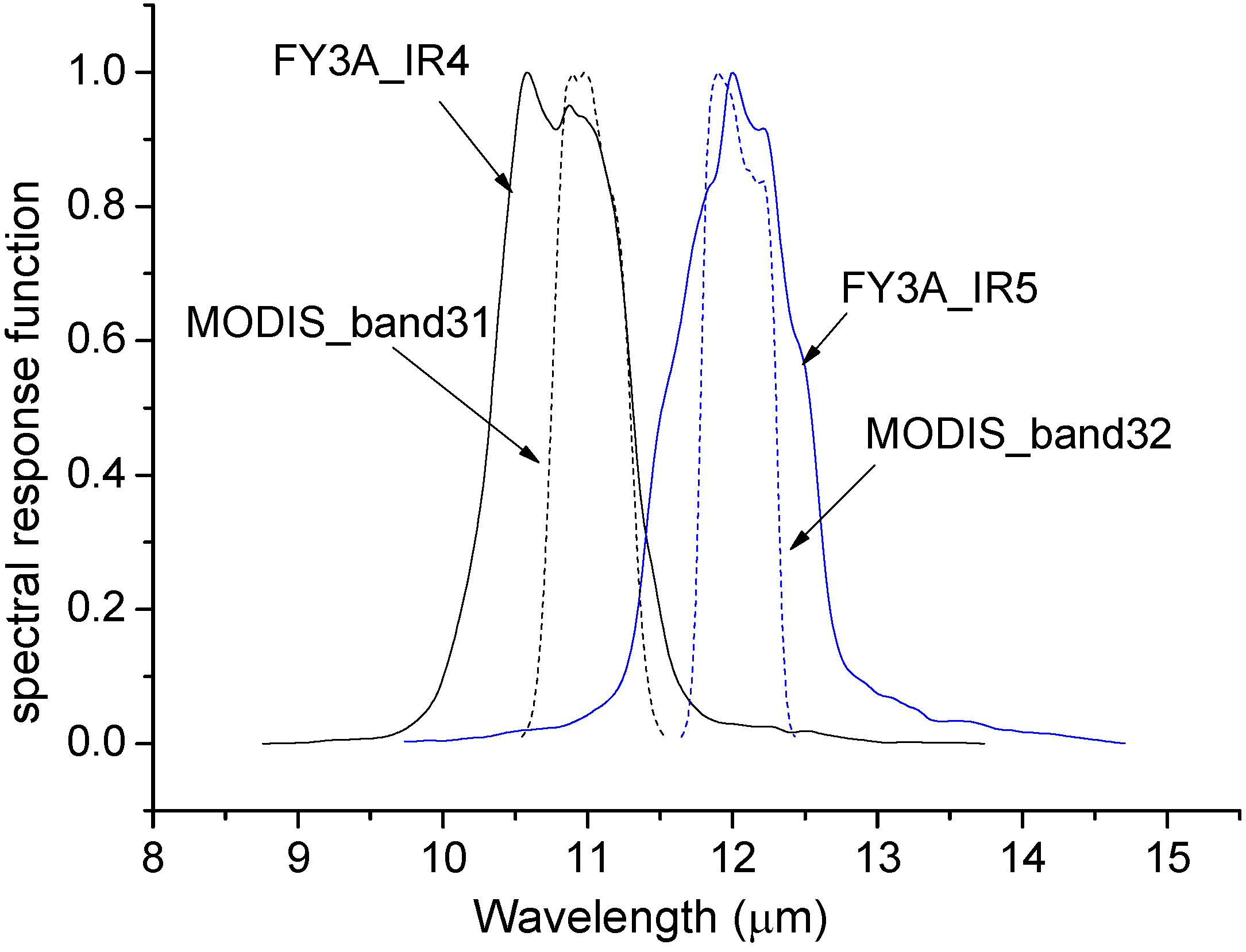
2.1. FY-3A Satellite Data

FengYun-3A (FY-3A) was launched on 27 May 2008, by the Taiyuan Launch Center, China. The second-generation polar-orbiting meteorological satellite carries ten payloads of optical and microwave sensors to collect a range of remote sensing data. The missions are meteorological forecasting, environmental change evaluation, natural disaster monitoring, etc. One of the major sensors is the Visible and Infrared Radiometer (VIRR), which includes seven visible and near-infrared channels and three infrared channels. The channel wavelengths of the instrument are depicted in Table 1.
The thermal-infrared Channels 4 (centered at 10.8 µm) and 5 (centered at 12.0 µm) data observed by the VIRR at the TOA were used to estimate the LST, and the seven visible and near-infrared channels were used to determine the LSE in this work.
Table 1. Specifications of the VIRR channels: spectral ranges and spatial resolutions. IFOV, instantaneous field of view; NEΔT, noise-equivalent temperature difference.
Channel No.Spectral Range (µm)IFOV (km)NE Δρ (%) NE ΔT (300 K)Dynamic Range (ρ or T)
10.58–0.681.10.1%0%–100%
20.84–0.891.10.1%0%–100%
33.55–3.931.10.3 K180–350 K
410.3–11.31.10.2 K180–330 K
511.5–12.51.10.2 K180–330 K
61.55–1.641.10.15%0%–90%
70.43–0.481.10.05%0%–50%
80.48–0.531.10.05%0%–50%
90.53–0.581.10.05%0%–50%
101.325–1.3951.10.19%0%–90%

2.2. MODIS Satellite Data

MODIS is a sensor aboard the NASA Earth Observing System (EOS) Terra satellite launched in 1999 and Aqua satellite launched in 2002. The passive imaging spectroradiometer consists of 36 spectral channels covering the visible and infrared wavelengths, from approximately 0.4 to 14.0 µm [30]. MODIS is intended to satisfy a diverse set of atmospheric, oceanographic and terrestrial science observational requirements. The data used in this work are the MOD11_L2, MOD03 and MCD12Q1 products provided by NASA Goddard Space Flight Center (GSFC) Level 1, the Atmosphere Archive and Distribution System (LAADS) [31] and the NASA-developed EOS Clearinghouse (ECHO) [32].
MOD11_L2 is an LST/LSE product that retrieves the LST from a generalized split-window algorithm [10], and LSEs are determined for Channels 31 and 32 via the classification-based emissivity method [33] at a 1-km spatial resolution. The LST product is used to cross-validate the LST estimated from the FY-3A VIRR data. MOD03 is the geolocation field data that are calculated for each 1-km MODIS instantaneous field of view (IFOV) for all daytime orbits. The geodetic latitude, longitude and satellite zenith angle of the geolocation fields are used in the inter-comparison. MCD12Q1, the MODIS land cover type yearly level 3 (L3) global 500-m sine (SIN) grid product, is classified by the International Geosphere-Biosphere Programme (IGBP) 17-class scheme [34]. This product is combined with the MOD11_L2 LST product to cross-validate the estimated VIRR LSTs for different land cover types.

2.3. In Situ Measurements

Experimental campaigns were conducted at the Hailar field site in Northeastern Inner Mongolia, China (49°21′N, 120°07′E). Figure 1 shows the location of the study site. The central area of the experiment is approximately 0.4 km2. The area has a cold temperate, semi-humid and semi-arid continental monsoon climate with a mean annual temperature of −2 °C and a mean annual rainfall of approximately 350 mm. The field site is a homogenous area fully covered by grasses and crops.
To ensure that the ground measurements of LST are representative at the satellite pixel scale, four infrared radiometers, SI-111, commercialized by Apogee Instruments, Inc., Roseville, CA, USA, were uniformly installed at an interval of 120 m at the field site. SI-111 measures thermal-infrared radiance in the 8.0–14.0 µm range and obtains brightness temperatures with an absolute accuracy of ±0.2 K. The sensors with a field of view (FOV) of 44° were mounted at a 2.0-m height to observe an area of approximately 2.0 m2. An additional SI-111 faces the sky at 53° with respect to the zenith and measures the spectral downwelling longwave radiance, which is used to correct for the reflected atmospheric component [35]. All station measurements recorded every 10 s were stored as one-minute averages from October, 2013, to September, 2014. In addition, to reduce the influence of the external environment on the measured infrared radiance, a wireless net observation system was adopted to transfer the radiances to a computer terminal.
Figure 1. Location of the study site (the four red points in the red rectangle show the locations of the installed infrared radiometers).
Remotesensing 07 03250 g001

3. Methodology

3.1. Radiative Transfer for the Split-Window Algorithm

Based on radiative transfer theory, for a cloud-free atmosphere in thermodynamic equilibrium, the channel radiance B i ( T i ) measured at the TOA in the TIR channel is approximately [36]:
B i ( T i ) = ε i B i ( T s ) τ i + R a t m _ i + ( 1 ε i ) R a t m _ i τ i
where T i is the channel brightness temperature observed in channel i at the TOA, B i is the Planck function, B i ( T i ) is the radiance emitted by a blackbody at temperature T s (i.e., LST; hereafter, LST is used interchangeably with T s ), ε i (i.e., LSE; hereafter, ε i is used interchangeably with LSE) is the channel emissivity in channel i, τ i is the total atmospheric transmittance along the target to the sensor path in channel i, R a t m _ i is the thermal-path atmospheric upwelling radiance in channel i and R a t m _ i is the channel downwelling atmospheric radiance from the entire hemisphere in channel i divided by pi. It is possible to obtain an expression for LST if Equation (1) is applied to two adjacent channels in one atmospheric window. This two-channel technique is based on the fact that the atmospheric attenuation due to the radiation emitted by the surface is proportional to the difference between the at-sensor radiances measured simultaneously in two infrared channels [10,37,38,39].

3.2. Algorithm Development for FY-3A VIRR Data

To develop an LST retrieval algorithm for FY-3A VIRR data, the atmospheric radiative transfer model, MODTRAN 4 [40], was used to simulate at-sensor radiance with the appropriate thermal-infrared channel response function of the VIRR. Figure 2 shows the corresponding spectral response functions of the FY-3A VIRR channels. For comparison, the spectral response functions of MODIS TIR Channels 31 (centered at 11.0 µm) and 32 (centered at 12.0 µm) are also shown in this figure.
Figure 2. Spectral response functions of FengYun-3A (FY-3A) VIRR Channels 4 and 5 and MODIS Channels 31 and 32.
Remotesensing 07 03250 g002
To broaden atmospheric variations to cover all possible real situations, two radiosonde observation databases are considered. One database is the latest version of the Thermodynamic Initial Guess Retrieval (TIGR), i.e., TIGR2002, which was constructed by the Laboratoire de Meteorologie Dynamique (LMD) to represent a worldwide set of atmospheric situations (2311 radio soundings) from polar to tropical atmospheres with varying water vapor amounts (0.1 to 8.0 g/cm2) and varying atmospheric surface temperatures (231 K to 315 K) [41]. The other database is the six standard atmospheric profiles for the tropics, mid-latitude summer, mid-latitude winter, sub-arctic summer, sub-arctic winter and 1976 United States standard atmosphere (US76) in MODTRAN 4. Because we only accounted for atmospheric variation in clear-sky conditions for LST retrievals, the TIGR2002 profiles with a relative humidity (RH) greater than 90% are discarded, considering that this high RH seldom occurs under clear-sky conditions. In addition, the profiles with a low-level warm layer that is more than 10 K warmer than the surface are also discarded, because the inversion could cause a negative atmospheric correction when used in the split-window technique [42]. Therefore, 1396 representative atmospheric situations in which the lowest atmospheric temperature T 0 ranges from 231 K to 315 K and WVC ranges from 0.06 g/cm2 to 6.44 g/cm2 are extracted from TIGR2002. In total, 1402 atmospheric profiles are used in our simulations.
Accounting for the angular dependence of the TOA radiance and the maximum VIRR viewing zenith angle (less than 65° from nadir), six viewing zenith angles (VZAs) (0°, 33.56°, 44.42°, 51.32°, 56.25° and 60°), corresponding to secant (VZA) = 1.0, 1.2, 1.4, 1.6, 1.8 and 2.0, respectively, are used in the MODTRAN simulations. Using the VZAs and the radio soundings mentioned above as MODTRAN input, we can obtain the channel atmospheric parameters ( τ i , R a t m _ i , R a t m _ i ) with spectral integration of the channel response function for each VZA and each atmospheric profile.
For a more realistic simulation, the LSTs are reasonably varied according to the atmospheric temperature T 0 in the lowest layer of the atmospheric profiles. Specifically, the LST varies from T 0 5 K to T 0 + 15 K in steps of 5 K for T 0 290 K and from T 0 5 K to T 0 + 5 K in steps of 5 K for T 0 < 290 K. Moreover, considering most land cover types, an average emissivity ε ¯ between 0.90 and 1.0 (a 0.02 interval) and an emissivity difference Δε between −0.02 and 0.02 (a 0.005 interval) exist for VIRR Channels 4 and 5 [10]. To demonstrate the assumption of emissivity, Figure 3 shows the emissivities of VIRR Channels 4 and 5 and the range of the emissivity difference Δε between the two TIR channels, as calculated from 146 spectrum samples of soil, vegetation, water and snow in the University of California Santa Barbara (UCSB) spectral database [43] and the Johns Hopkins University (JHU) [44] spectral database.
Figure 3. Value of emissivity and range of emissivity differences between VIRR Channels 4 and 5. JHU, Johns Hopkins University; UCSB, University of California Santa Barbara.
Remotesensing 07 03250 g003
For a given LST, in combination with the atmospheric parameters ( τ i , R a t m _ i , R a t m _ i ), T s and ε i , the channel brightness temperature T i (i = 4, 5) at the TOA can be determined according to Equation (1) with the inverse of Planck’s law. At this stage, T s is directly related to the TOA-measured brightness temperature T i (i = 4, 5). In total, for the TIGR2002 database, 257,256 situations represent the simulated database for the LST estimation and for calculating the regression coefficients; 1188 situations are obtained for the six standard MODTRAN 4 atmospheres to validate the present algorithm, for each VZA.
Figure 4 shows the relationship between T s T 4 and T 4 T 5 calculated for all of the above-mentioned conditions with six sub-ranges of WVC between 0 and 6.5 g/cm2; for a mean emissivity ε ¯ = 1, the emissivity difference Δε = 0, and VZA = 0°. From this figure, one can see that the relationship between T s T 4 and T 4 T 5 varies with the WVC sub-ranges. Therefore, the WVC should be divided into sub-ranges to retrieve the LST accurately. Based on Figure 4 and the non-linearity of the Planck function for temperature, a quadratic form is proposed [45,46,47]:
T s = a 0 + a 1 * T 4 + a 2 * ( T 4 T 5 ) + a 3 * ( T 4 T 5 ) 2
where T s is the land surface temperature with surface emissivity ε = 1; T 4 and T 5 are the TOA brightness temperatures of FY-3A VIRR Channels 4 and 5, respectively; and a 0 a 3 are the coefficients as functions of the WVC and VZA.
Figure 4. Relationship between T s T 4 and T 4 T 5 calculated for all of the above-mentioned conditions with six sub-ranges of water vapor content (WVC) between 0 and 6.5 g/cm2; for a mean emissivity ε = 1, the emissivity difference Δε = 0, and the viewing zenith angle (VZA) = 0°.
Remotesensing 07 03250 g004
Figure 5 presents the histograms of the difference between the actual and estimated T s (Equation (2)) for the WVC sub-range [0, 1.5] and VZA = 0° and the WVC sub-range [5.5, 6.5] and VZA = 60°. The root mean square error (RMSE) between the actual and estimated T s is 0.11 K for the former sub-range and 2.53 K for the latter sub-range at a surface emissivity ε = 1 and emissivity difference Δε = 0. The RMSEs obtained for the other WVC sub-ranges and VZAs are between these two values.
Not all of the radiation sources at the Earth’s surface are blackbodies with emissivities equal to one. The most common land cover surface emissivity must be taken into account in the development of the split-window algorithm. Prata et al. [48] showed that a 1% emissivity uncertainty can affect LST values by approximately 0.7 K. Consequently, for different values of the numerical experiments mentioned above, as conducted by Wan and Dozier [10], the average emissivities are divided into two groups: 0.90 to 0.96 and 0.94 to 1.0. Note that the Planck function is a non-linear function of the LST. To obtain a nearly non-linear function with linear segments for accurately retrieving the LST, there must be some segment overlap. Therefore, the atmospheric WVCs are divided into six sub-ranges with an overlap of 0.5 g/cm2. The LSTs, T s , are divided into five sub-ranges with an overlap of 5 K. Details on the various intervals of WVC and LST are presented in Table 2. We then retrieve the LST by using a split-window algorithm as follows [49]:
T s = b 0 + b 1 * T 4 + b 2 * ( T 4 T 5 ) + b 3 * ( T 4 T 5 ) 2 + b 4 * ( 1 ε ¯ ) + b 5 * Δ ε
where b i (i = 0, 5) are coefficients, which can be obtained through statistical regressions for each VZA and each sub-range. ε ¯ is the average mean emissivity, and Δε is the emissivity difference between VIRR Channels 4 and 5. Note that the coefficient b i is determined by each VZA and each sub-range, so the estimation accuracy of the WVC does not need to be very high for retrieving an accurate LST. In practice, when the WVC or LST of a pixel is located in two adjacent sub-ranges, we first calculate the distances between the numerical value of the WVC/LST and the central values of the two sub-ranges. The coefficients in the sub-range with a shorter distance are used to retrieve the LST.
Figure 5. Histograms of the difference between the actual T s and the T s estimated using Equation (2) for (a) the WVC sub-range [0, 1.5] and VZA = 0° and (b) the WVC sub-range [5.5, 6.5] and VZA = 60°.
Remotesensing 07 03250 g005
Table 2. Tractable sub-ranges of WVC and LST to determine the regression coefficients in Equation (3).
VariableTractable Sub-RangeOverlap
Water vapor content (WVC) (g/cm2)[0, 1.5], [1.0, 2.5], [2.0, 3.5], [3.0,4.5], [4.0, 5.5], [5.0, 6.5]0.5
Land surface temperature (LST) (K)≤280, [275, 295], [290, 310], [305, 325], ≥3205.0
All of the numerical values of the coefficients given by Equation (3) can be determined through statistical regression for each VZA and each sub-range and can be stored in a look-up table. Table 3 lists, for example, the coefficients b 0 to b 5 of the split-window algorithm for the six VZAs in the WVC sub-range of 1.0 g/cm2 to 2.5 g/cm2 and the LST sub-range of 275 K to 295 K for the two emissivity groups. To determine the coefficient b 0 for other VZAs, we can linearly interpolate the six b 0 stored in the look-up table as a function of the secant VZA. Similar processes are used to determine the coefficients b 1 to b 5 for other VZAs.
Table 3. Coefficients of the split-window algorithm for the WVC sub-range of 1.0 g/cm2 to 2.5 g/cm2 and the LST sub-range of 275 K to 295 K for the two emissivity groups.
ConditionsWVC [1.0, 2.5] Ts [275 K, 295 K]
Emissivity1/cos(VZA)b0b1b2b3b4b5
ε [ 0.90 ,   0.96 ] 1.06.15890.97992.1183−0.081950.4947−97.6539
1.27.25450.97642.2088−0.070049.9067−97.4687
1.48.31960.97302.2919−0.057949.3379−97.0982
1.69.36400.96962.3681−0.045448.7807−96.5531
1.810.39500.96622.4369−0.032748.2272−95.8291
2.011.40440.96292.4995−0.019947.6776−94.9575
ε [ 0.94 ,   1.0 ] 1.03.86810.98891.8190−0.039547.9444−85.0717
1.24.54540.98691.9230−0.029747.5162−86.0962
1.45.18310.98502.0150−0.019747.0893−86.6894
1.65.79100.98312.0973−0.009446.6635−86.9527
1.86.37890.98142.17130.000946.2359−86.9394
2.06.94400.97972.23830.011345.8088−86.7118

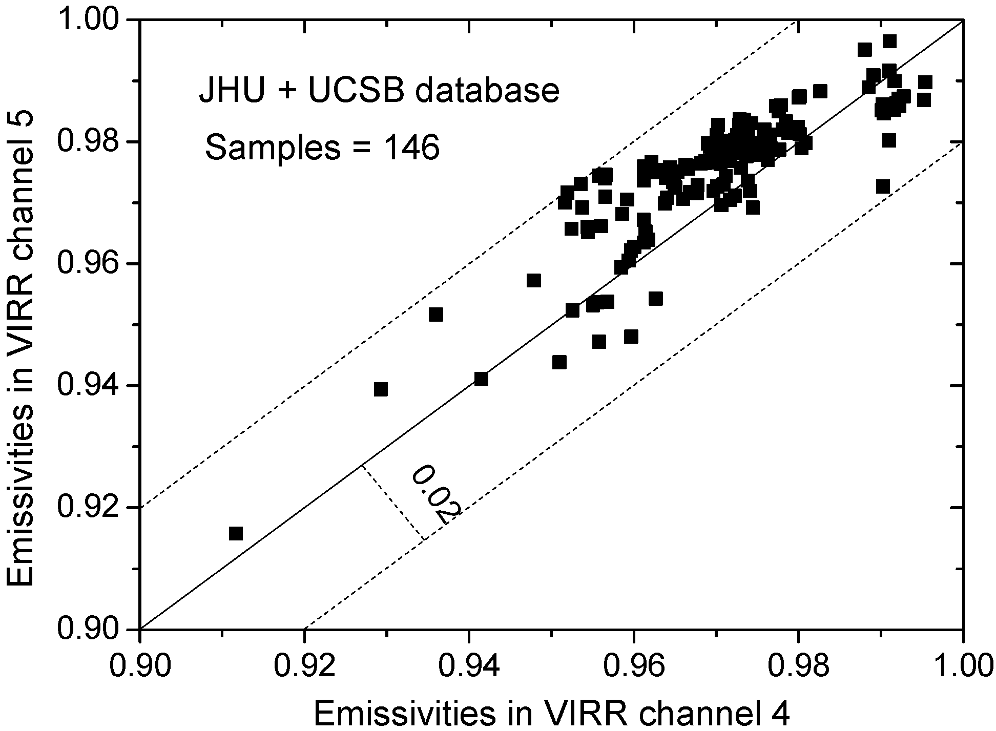
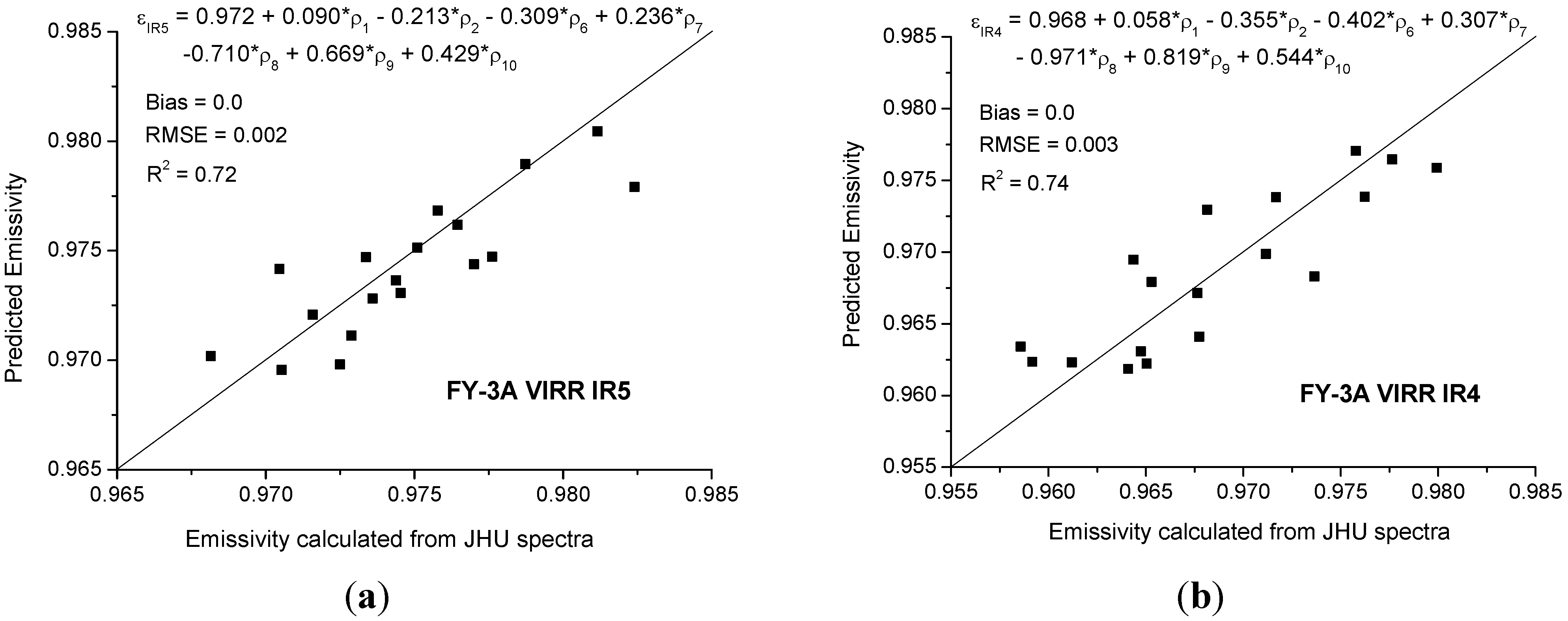
3.3. Determination of LSEs

As shown in Equation (3), the mean and differenced LSEs are model inputs. The accuracy of the retrieved LST also depends on the accuracy of the LSEs, particularly for dry atmospheric conditions. It is therefore preferable to determine the LSEs from the same sensors at the same spatial resolution. An NDVI-based threshold method [6] is adopted in this work. The normalized difference vegetation index (NDVI) is calculated as N D V I = ( ρ 2 ρ 1 ) / ( ρ 2 + ρ 1 ) , where ρ 1 and ρ 2 represent the FY-3A VIRR Channel Reflectances 1 (0.58–0.68 µm) and 2 (0.84–0.89 µm). The method determines the LSE according to the soil characteristics present in one pixel by considering the following cases.

3.3.1. Bare Soil Pixels

Sobrino and Raissouni [46] and Sobrino et al. [6] noted that a NDVI value of 0.2 for bare soil and 0.5 for full vegetation are appropriate for global applications of a 1-km remotely-sensed land dataset. Thus, pixels with NDVI values below 0.2 are considered bare soil in this work. In this case, the typical soil spectra from the Johns Hopkins University (JHU) [44] spectral library database are used to simulate the VIRR channel reflectances (1–2 and 6–10) and emissivities (4–5) by combining the spectral response functions of those channels. Seventeen samples with unique major soil types, including clay loam, silty loam, sandy loam and loamy sand, are used in this investigation. Two statistical relationships are obtained by correlating the emissivities in Channels 4 and 5 to the channel reflectances ( ρ j ) for the seven visible and near-infrared channels. The multiple linear regression relationships can be written as:
ε I R _ s i = c 0 i + j = 1 ~ 2 , 6 ~ 10 c i j ρ j           ( i = 4 , 5 )
where ε I R _ s i (i = 4, 5) are the bare soil emissivities for Channels 4 and 5, respectively. c is the regression coefficient. Figure 6 compares the estimated LSEs to the actual LSEs calculated from the JHU spectra database for various bare soil types. This figure shows that the emissivities for Channels 4 and 5 can be relatively well described using the visible and near-infrared channel reflectances. These fitting results exhibited RMSE (R-square) values between the actual and estimated emissivities: 0.003 (0.74) for Channel 4, and 0.003 (0.72) for Channel 5.
Figure 6. Comparisons of the estimated LSEs and the actual LSEs calculated from the JHU spectra database for different bare soil types.
Remotesensing 07 03250 g006

3.3.2. Fully Vegetated Pixels

Pixels with NDVI values above 0.5 are considered fully vegetated ( P v = 1) [6,46]. Because the United States Geological Survey (USGS) spectral library only provides reflectivity spectra and because the UCSB spectral library (University of California, Santa Barbara) only provides emissivity spectra, the JHU spectral library with both reflectivity and emissivity spectra for different surface types was used. Unfortunately, JHU only provides four vegetation spectra (conifer, broadleaf, green grass and dry grass), so all four vegetation spectra are used to simulate the VIRR channel reflectances (1–2) and channel emissivities (4–5). Two statistical relationships are obtained by correlating the Channel 4 and 5 emissivities ( ε I R _ v 4 and ε I R _ v 5 ) to the NDVI:
ε I R _ v 4   = 0.889 + 0.119 N D V I
ε I R _ v 5   = 0.894 + 0.116 N D V I
Comparing the estimated emissivities and the actual emissivities calculated from the JHU spectra database shows that the RMSEs (R-squares) are 0.006 (0.97) for Channel 4, and 0.007 (0.95) for Channel 5.

3.3.3. Mixed Pixels

When the NDVI value is between 0.2 and 0.5, the pixel is a mixture of bare soil and vegetation. The emissivity is calculated according to the proportion of the bare soil to the vegetation [6]:
ε I R _ v i P v + ε I R s i ( 1 P v ) + C i         ( i = 4 ,   5 )
The vegetation proportion, P v , is calculated by [50]:
P v = [ N D V I N D V I m i n N D V I m a x N D V I m i n ] 2
where N D V I m i n = 0.2 and N D V I m a x = 0.5 . The term C i includes the effect of the geometrical distribution on the natural surfaces and the internal reflections (cavity effect) (i.e., for homogeneous and flat surfaces C i =0). A good approximation for this term is given by:
C i = ( 1 ε I R _ s i ) ( 1 P v ) F ε I R _ v i         ( i = 4 ,   5 )
where F is a shape factor [6], whose mean value is assumed to be 0.55 for VIRR Channels 4 and 5. ε I R _ s i and ε I R _ v i are obtained using Equations (4)–(6), respectively.

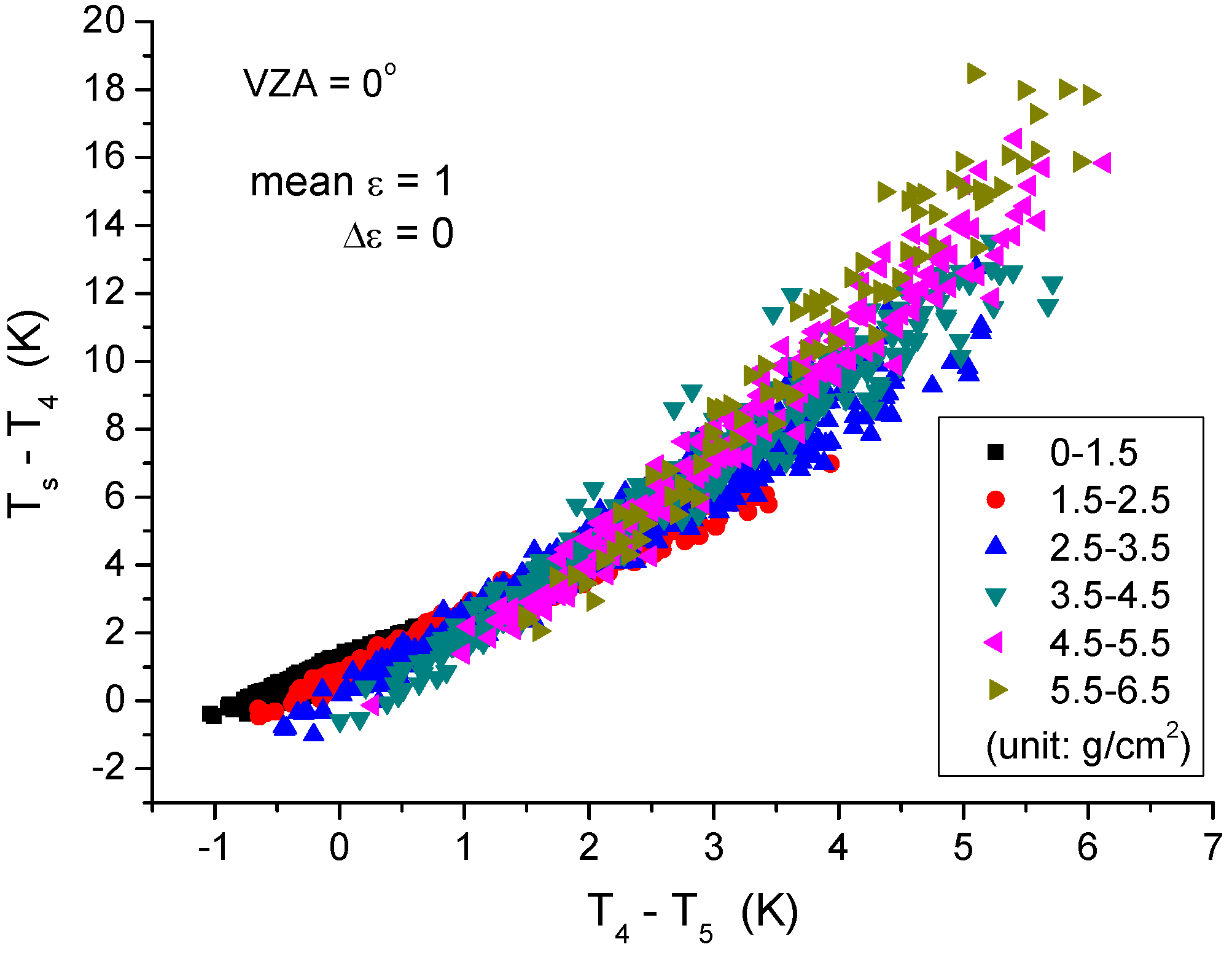
3.4. Determination of Atmospheric WVC

Considering that the WVC is used to determine the optimal coefficients in the LST algorithm, an accurate WVC is not required provided that the estimated WVC is within the same sub-range as the actual WVC. The method proposed by [51], which utilizes the transmittance ratio of two split-window channels to derive the WVC, is used:
W V C = d 1 + d 2 × τ j τ i
τ j τ i = ε i ε j R j i
and:
R j i = k = 1 N ( T i , k T ¯ i ) ( T j , k T ¯ j ) k = 1 N ( T i , k T ¯ i ) 2
where d 1 and d 2 are unknown coefficients; τ i and τ j are the atmospheric transmittances in the split-window channels i and j, respectively; the subscript k denotes pixel k; and T ¯ i and T ¯ j are the TOA mean (or the median) channel brightness temperatures of the N neighboring pixels considered for channels i and j, respectively.
Based on the numerical simulated results of τ i and τ j obtained in Section 3.2, coefficients d 1 and d 2 are first determined by Equation (10) and are further derived as functions of the secant VZA:
d 1 = 25.156 13.572 / cos ( V Z A ) + 2.909 / cos 2 ( V Z A )
d 2 = 25.258 + 13.677 / cos ( V Z A ) 2.931 / cos 2 ( V Z A )
The results of the comparison between the actual input WVC for the MODTRAN simulations and the WVC estimated by Equations (10) and (13)–(14) show that the bias and RMSE are 0.08 g/cm2 and 0.16 g/cm2, respectively, which indicate that the estimated WVC can meet the needs of the proposed LST retrieval algorithm.

4. Results and Discussion

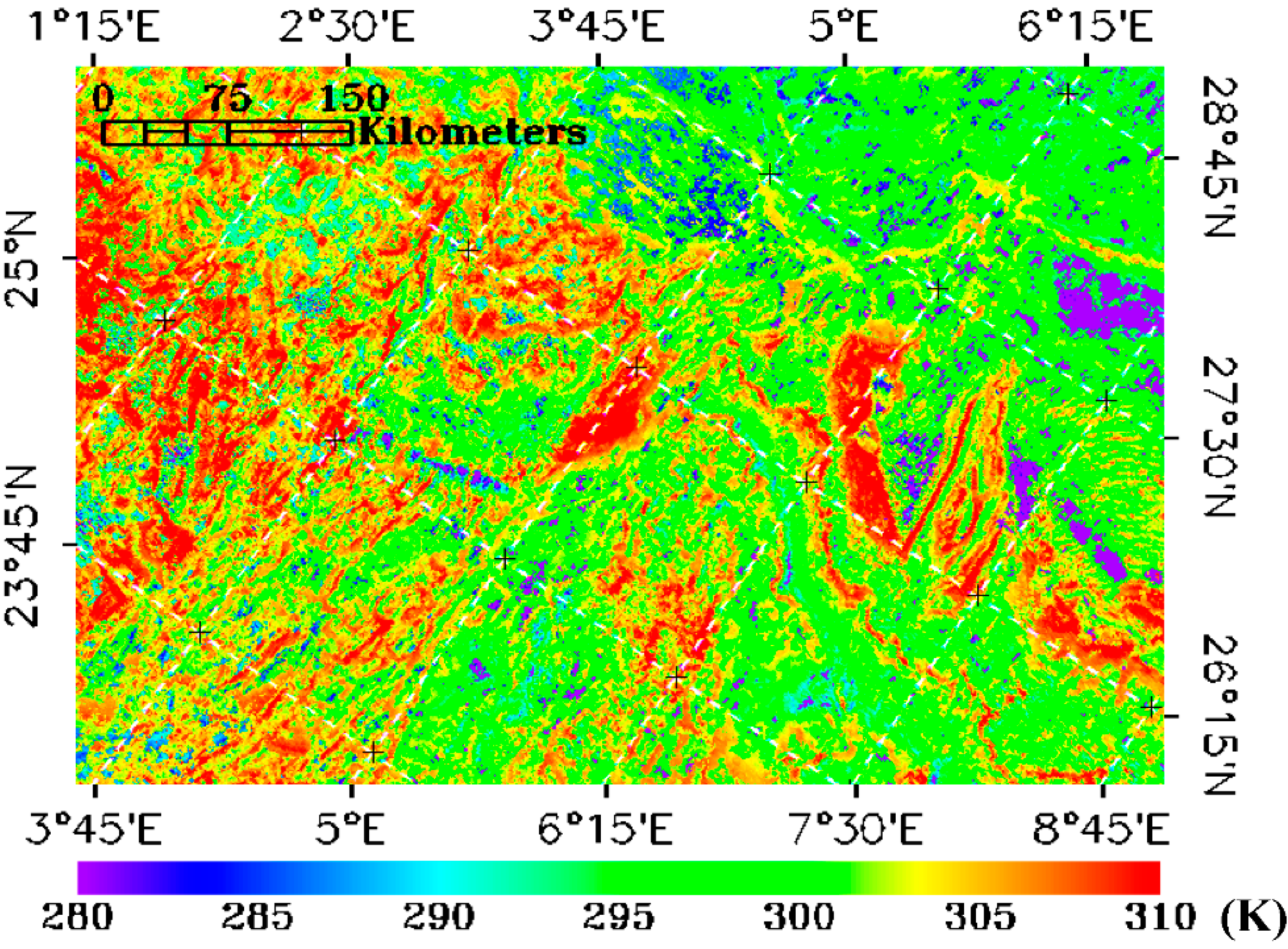
4.1. Estimation of LST

Figure 7 shows the histogram of the difference between the actual T s and the T s estimated with the coefficients corresponding to the sub-range W V C [ 1.0 ,   2.5 ] and T s [ 275   K ,   295   K ] for two emissivity groups and VZA = 0°. The RMSE between the actual and estimated T s is 0.28 K for the emissivity group ε [ 0.94 ,   1.0 ] and 0.37 K for the other emissivity group ε [ 0.90 ,   0.96 ] .
Figure 7. Histogram of the difference between the actual and estimated T s for the WVC sub-range of 1.0 g/cm2 to 2.5 g/cm2 and the LST sub-range of 275 K to 295 K for VZA = 0°. (a) ε [ 0.90 ,   0.96 ] and (b) ε [ 0.94 ,   1.0 ] .
Remotesensing 07 03250 g007
In addition, Figure 8 presents the RMSEs between the actual and estimated T s as functions of the secant VZA for the two emissivity groups with different sub-ranges. Considering that, in reality, a lower LST is usually accompanied by low WVC, for the LST less than 280 K, the maximum WVC is 2.5 g/cm2. For the LST between 275 K and 295 K, the maximum WVC is 5.5 g/cm2.
As seen from Figure 8, the RMSEs increase as the VZA increases. The RMSEs are below 1 K for all sub-ranges of VZA below 30° or for all sub-ranges of VZA below 60° and WVC below 3.5 g/cm2. The RMSEs increase dramatically with the increase in the VZA when the WVC is above 3.0 g/cm2, with a maximum RMSE of 2.5 K for the sub-range ε [ 0.94 ,   1.0 ] , W V C [ 5.0 ,   6.5 ] and T s [ 305   K , 325   K ] for VZA = 60°.
Note that, in practice, the LST is estimated in two steps for actual satellite data. First, the approximate LSTs are estimated using Equation (3) with the coefficients derived for the entire range of LST provided that the sub-ranges of the emissivity and WVC are known; then, more accurate LSTs are estimated again using Equation (3), but with the coefficients b 0 b 5 corresponding to the sub-range of LST, which is determined according to the approximate LST obtained in the first step. Figure 8 also shows the RMSEs between the actual T s and the T s estimated with the coefficients obtained for the entire range of LSTs.
Figure 8. RMSEs between the actual and estimated T s as functions of the secant VZA for various sub-ranges in two emissivity groups.
Remotesensing 07 03250 g008

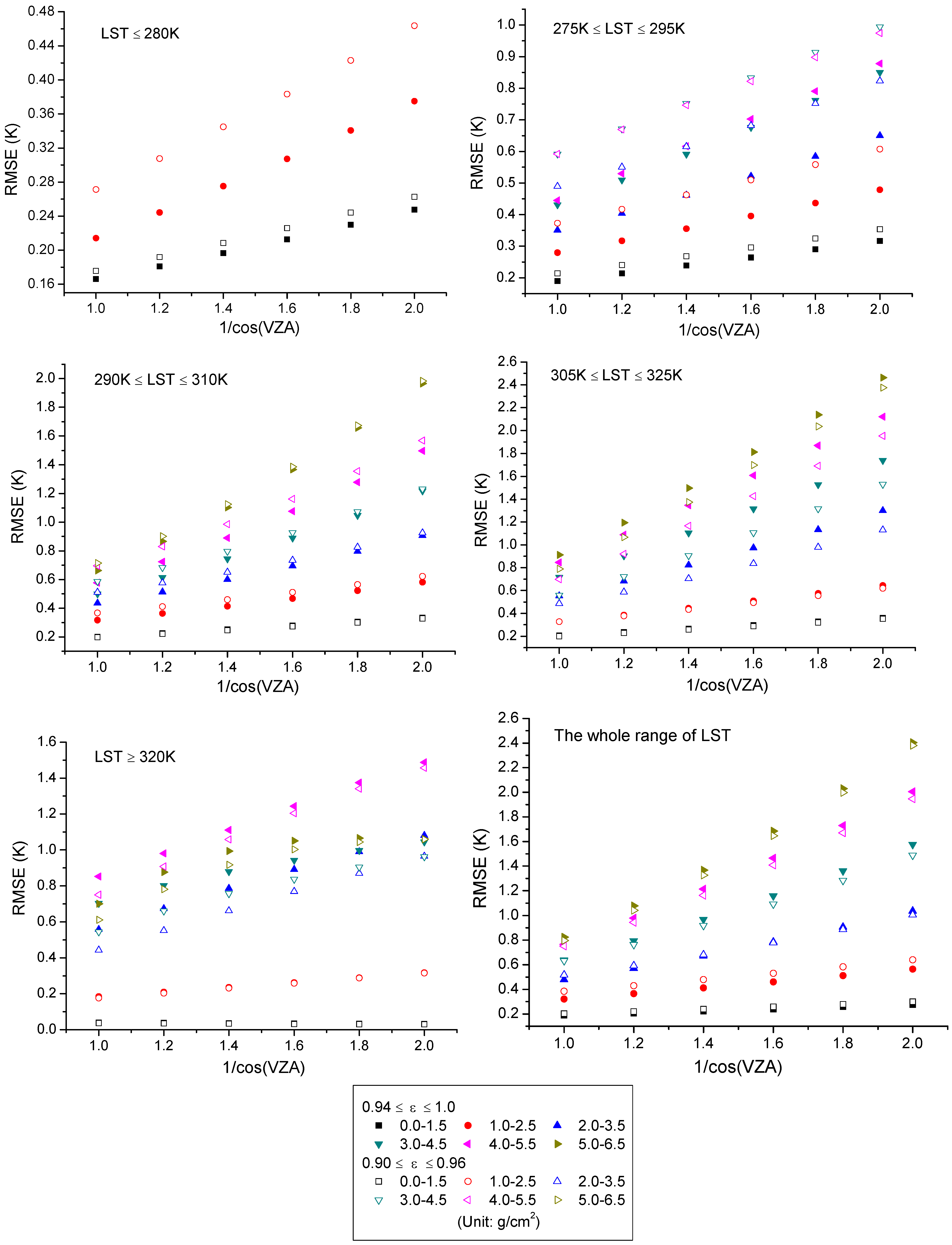
4.2. Sensitivity Analysis

As Wan and Dozier [10] noted, the errors in the LST estimated by the split-window algorithm mainly result from the uncertainties in instrument noise, atmospheric properties and LSEs. These three sources of uncertainties are analyzed below.

4.2.1. Instrument Noise (NEΔT)

The noise-equivalent temperature differences (NEΔT) for FY-3A VIRR Channels 4 and 5 are both 0.2 K, as specified in Table 1. To determine the significance of the instrument NEΔT on the retrieval of LST, a Gaussian random distribution error of 0.2 K is added to the simulated TOA brightness temperatures T 4 and T 5 in Equation (3). We then estimate the LST using Equation (3) with the noisy TOA brightness temperatures and compare it to the actual LST. For ε [ 0.94 ,   1.0 ] , W V C [ 1.0 ,   2.5 ] and T s [ 275   K ,   295   K ] , as an example, the effect of the instrument NEΔT on the LST retrieval is small, with an RMSE of 0.34 K. In contrast to the RMSE of 0.28 K for no-noise cases, the retrieval accuracy of the LST is changed by 21% for NEΔT = 0.2 K.

4.2.2. Land Surface Emissivity

From Equation (3), one can see that the accuracy of the LST retrieval related to the LSE is mainly dependent on the uncertainties in ( 1 ε ¯ ) and Δε. The LST error σ L S T due to the uncertainty in ( 1 ε ¯ ) and Δε can be estimated by:
σ L S T = b 4 2 σ ( 1 ε ) 2 + b 5 2 σ ( Δ ε ) 2
where b 4 and b 5 are the regression coefficients obtained in Section 3.2. For T s [ 275   K ,   295   K ] and W V C [ 1.0 ,   2.5 ] for two emissivity groups at VZA = 0, as an example, and assuming that the uncertainties in ( 1 ε ¯ ) and Δε are approximately 1%, we can obtain an LST error of 0.97 K for the high emissivity group ε [ 0.94 ,   1.0 ] and 1.1 K for the low emissivity group ε [ 0.90 ,   0.96 ] .

4.2.3. Atmospheric WVC

It is well known that the WVC is not easily determined from satellite data. Note that the WVC is divided into six sub-ranges with an overlap of 0.5 g/cm2 in the present spilt-window algorithm. The WVC overlap can be divided into two adjacent sub-ranges. Specifically, the two sub-ranges correspond to two pairs of coefficients b 0 b 5 . Therefore, the effect of the uncertainty in the WVC on the LST retrieval is mainly due to the incorrect sub-range selection of the WVC. In this work, we aim to analyze the effect of the WVC overlap on the LST retrieval. The WVC overlap for W V C [ 1.0 ,   1.5 ] in the high emissivity group ε [ 0.94 ,   1.0 ] can be divided into two sub-ranges: W V C [ 0.0 ,   1.5 ] and W V C [ 1.0 ,   2.5 ] . We first estimate the LST with W V C [ 1.0 ,   1.5 ] using the coefficients corresponding to the sub-ranges ε [ 0.94 ,   1.0 ] , W V C [ 0.0 ,   1.5 ] and T s [ 275   K ,   295   K ] ; the RMSE between the actual and the estimated LST is 0.21 K. When using the coefficients corresponding to the sub-ranges ε [ 0.94 ,   1.0 ] , W V C [ 1.0 ,   2.5 ] and T s [ 275   K ,   295   K ] , the RMSE is 0.26 K. This result shows that the uncertainty in the WVC can affect the accuracy of the LST retrieval by 24%.

4.2.4. Total Error

The total maximum error is calculated according to the expression given by:
σ t o t a l 2 = σ R M S E 2 + σ n o i s e 2 + σ ε 2 + σ W V C 2
where σ t o t a l is the total error associated with the proposed split-window algorithm, σ R M S E is the error caused by the proposed algorithm itself, σ n o i s e is the error related to the instrument noise, σ ε is the error with respect to LSE and σ W V C is the error caused by the uncertainty in the atmospheric WVC. For the sub-ranges ε [ 0.94 ,   1.0 ] , W V C [ 1.0 ,   2.5 ] and T s [ 275   K ,   295   K ] , the retrieval accuracy of the LST related to the algorithm is affected by 0.28 K. The errors caused by the instrument noise, LSE and the uncertainty in the atmospheric WVC are 0.21, 0.97 and 0.24 K, respectively. Finally, the total error associated with the LST retrieval is approximately 1.1 K.

5. Validation

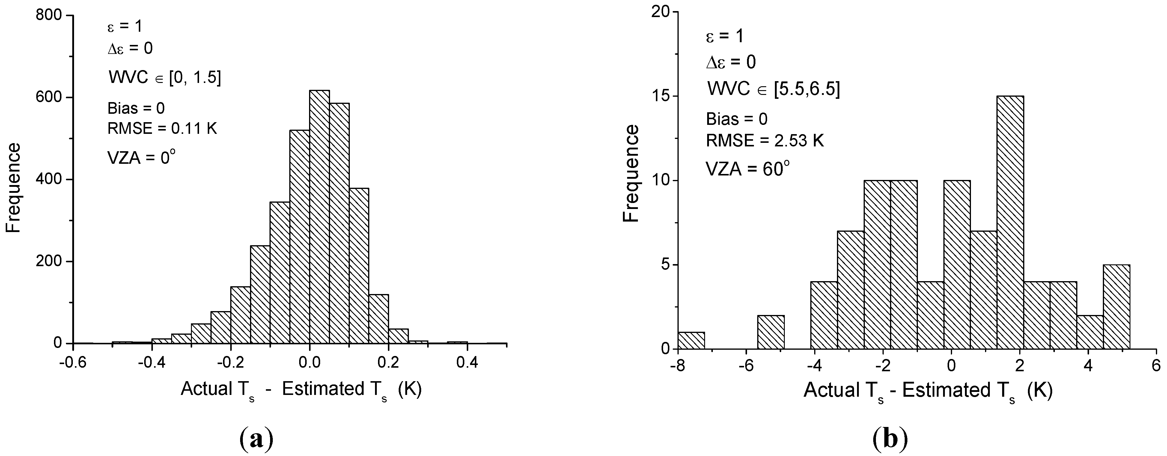
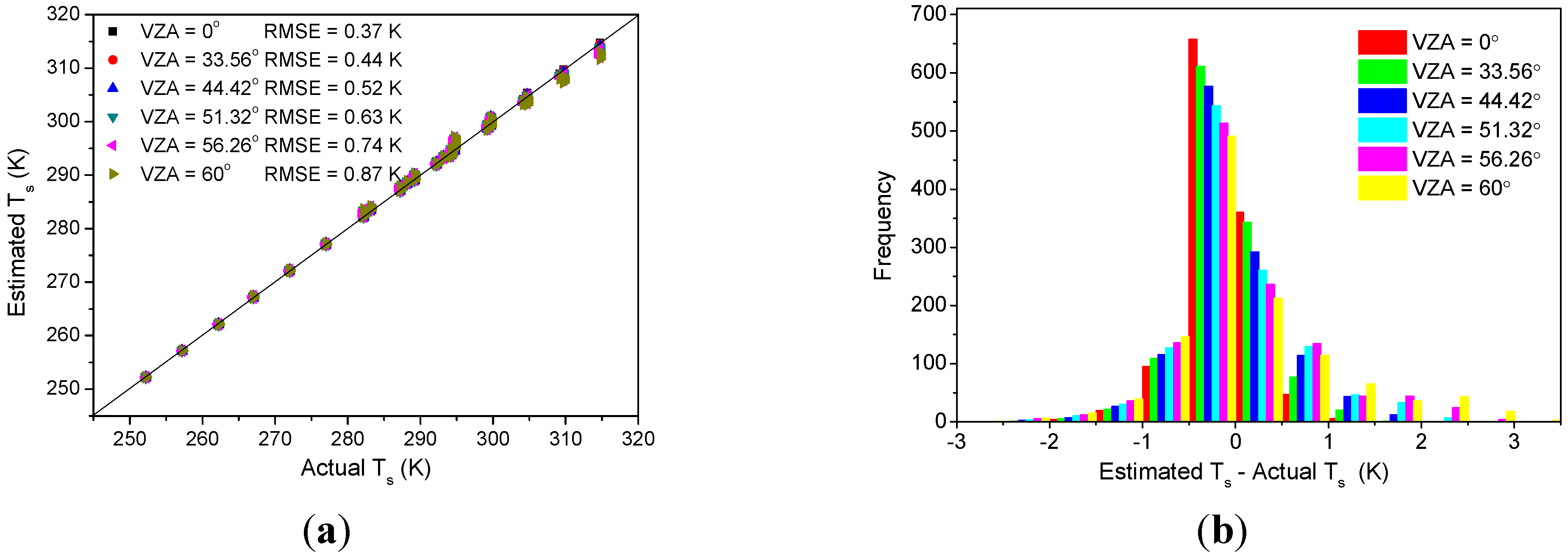
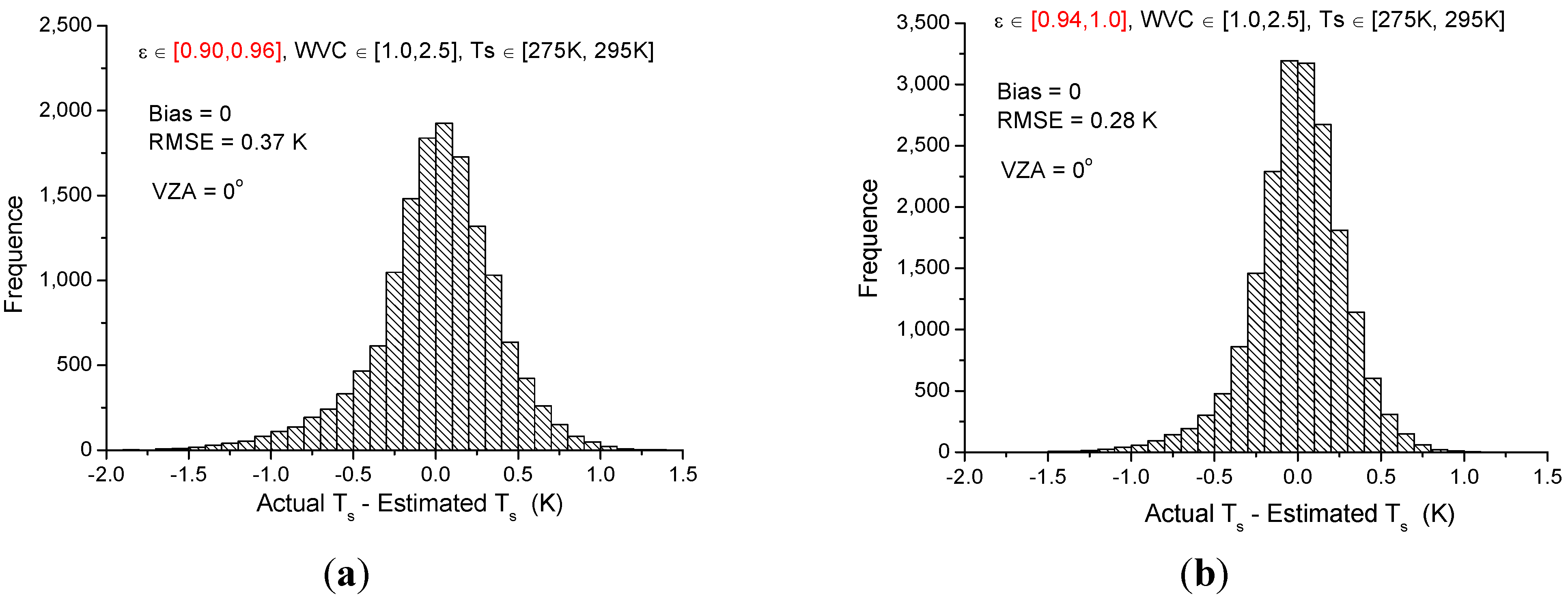
5.1. Validation Using the Simulated Data

To test the performance of the proposed algorithm, data simulated with the same viewing geometry and land surface type conditions, but with the six standard atmospheres provided by MODTRAN 4, as mentioned in Section 3.2, are used. The TOA brightness temperatures for VIRR Channels 4 and 5 are obtained in combination with the MODTRAN outputs of the atmospheric parameters ( τ i , R a t m _ i , R a t m _ i ) and reasonable variations in the T s and ε i . We then calculate the surface temperature using the proposed split-window algorithm. Figure 9 shows a comparison and difference histogram of the actual T s and the estimated T s using the proposed algorithm for different types of surfaces and atmospheric profiles. The RMSEs listed in this figure stem from estimating the LST at various VZAs. The results are quite consistent with the maximum RMSE below 1 K.
Figure 9. Comparisons (a) and difference histogram (b) of the actual LSTs (i.e., the MODTRAN 4 input LSTs) and those estimated using the proposed split-window algorithm for different types of surfaces, the six standard atmospheric profiles and the different VZAs.
Remotesensing 07 03250 g009

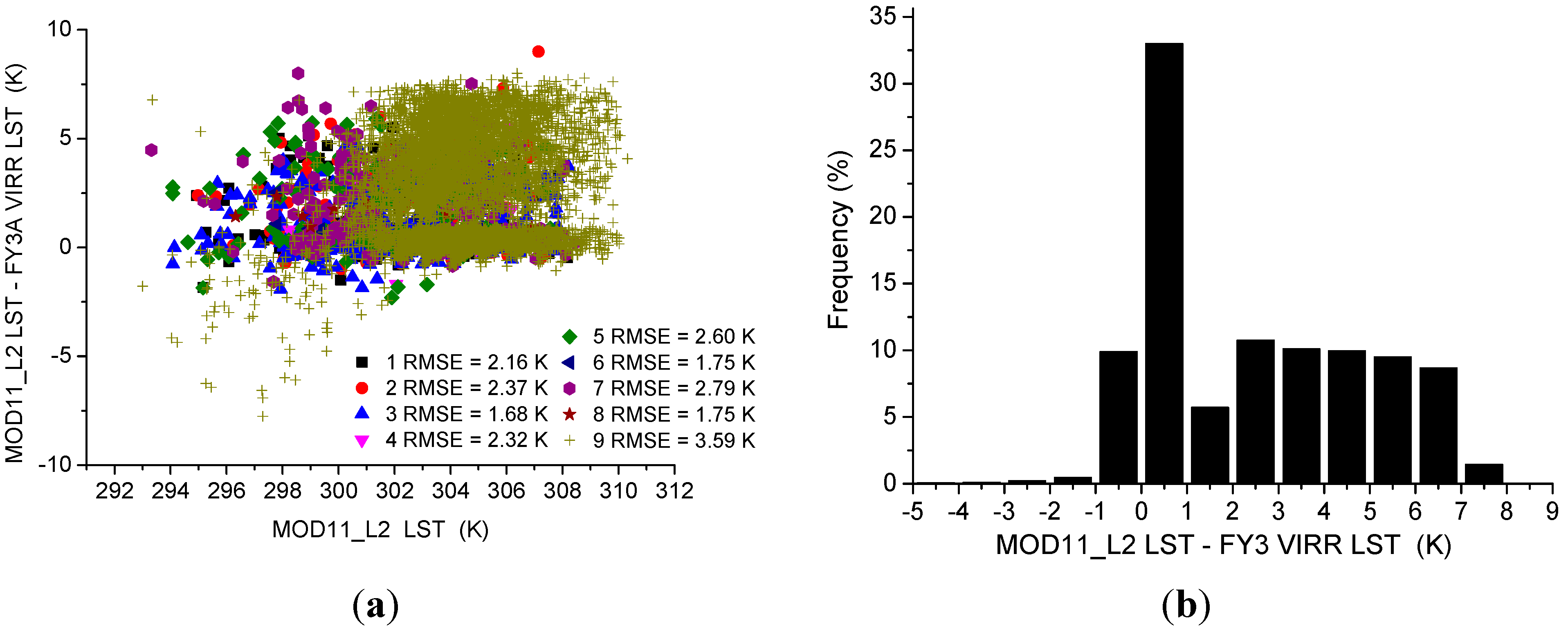
5.2. Validation Using the MODIS LST Product MOD11_L2

An inter-comparison method using the MODIS-derived validated LST V5 product MOD11_L2 at a 1-km resolution is used to validate the proposed LST retrieval algorithm. Considering that the LST at the satellite pixel scale rapidly varies with high spatiotemporal variations, the accuracy of the inter-comparison method depends on the geographic coordinate matching, temporal matching and VZA matching of the two satellite-derived LST products [1,24,25].
Considering that the spatial resolutions for VIRR and MODIS are 1.1 km and 1 km, respectively, we do not take into account the spatial difference between these two estimated LSTs. The LSTs estimated using the proposed method from FY-3A VIRR data are resampled to a 1-km resolution according to the nearest-neighbor interpolation method. To avoid the effect of different view times on the LST difference between MODIS and VIRR, a region over which both sensors pass at the same time is chosen, i.e., Algeria (22.705°N to 29.145°N and 1.173°E to 9.047°E). The observation time of the two sensors is 10:30 UTC, 5 January 2010. Figure 10 gives the map of LST estimated from FY-3A VIRR satellite data for this inter-comparison region.
Figure 10. Map of LST estimated from FY-3A VIRR satellite data at the observation time of 10:30 UTC, 5 January 2010.
Remotesensing 07 03250 g010
To reduce the effect of different viewing zenith angles, the pixels with VZA differences of less than 10° are considered. Figure 11 displays the differences between the MOD11_L2 LSTs and FY-3 VIRR LSTs as a function of MOD11_L2 LSTs and the corresponding histogram. The different RMSEs are calculated according to the different land cover types, which are obtained from the MODIS land cover type 2010 L3 global 500-m SIN grid product MCD12Q1 and are classified by the International Geosphere-Biosphere Programme (IGBP) 17-class scheme [34]. To match the MODIS and VIRR LSTs, the 500-m SIN grid data are projected onto a 1-km Albers equal area projection using the MODIS Reprojection Tool (MRT) [52]. Compared with MOD11_L2 LST, the proposed method underestimates the VIRR LST, with an RMSE of 2.16 K for a cropland/natural vegetation mosaic, 2.37 K for croplands, 1.68 K for grassland, 2.32 K for open shrub land, 2.60 K for permanent wetlands, 1.75 K for savannas, 2.79 K for urban and built-up land, 1.75 K for woody savannas and 3.59 K for barren or sparsely vegetated surfaces. Therefore, the difference between two estimated LSTs is relative small for homogeneous land surfaces, such as grasslands, while the difference is large for heterogeneous land surfaces, particularly barren or sparsely vegetated land cover. Note that spatial and angular differences exist between MODIS and VIRR and somewhat affect the resultant LSTs for comparison. In addition, as shown in Figure 2, the differences between the two TIR spectral response functions are relative large, and the calibration difference between the two sensors also affects the LST comparison.
Figure 11. Comparison of two LSTs: (a) the difference between MOD11_L2 and VIRR LSTs as a function of MOD11_L2 LST; and (b) the corresponding histogram of the LST differences (1, cropland/natural vegetation mosaic; 2, croplands; 3, grassland; 4, open shrub land; 5, permanent wetlands; 6, savannas; 7, urban and built-up land; 8, woody savannas; 9, barren or sparsely vegetated).
Remotesensing 07 03250 g011

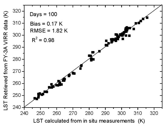
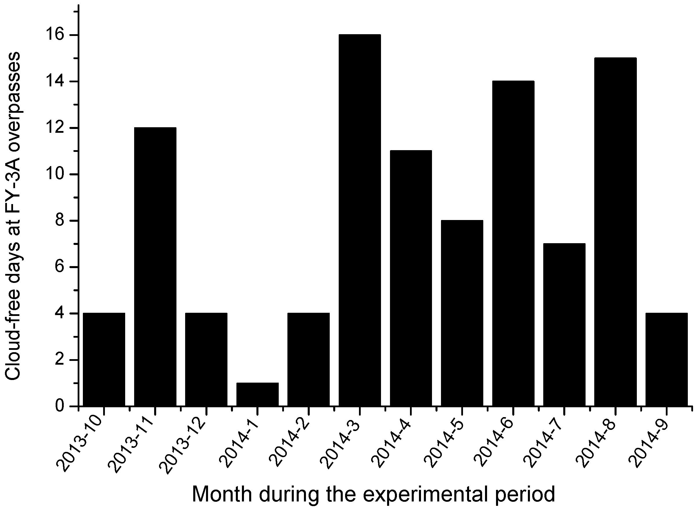
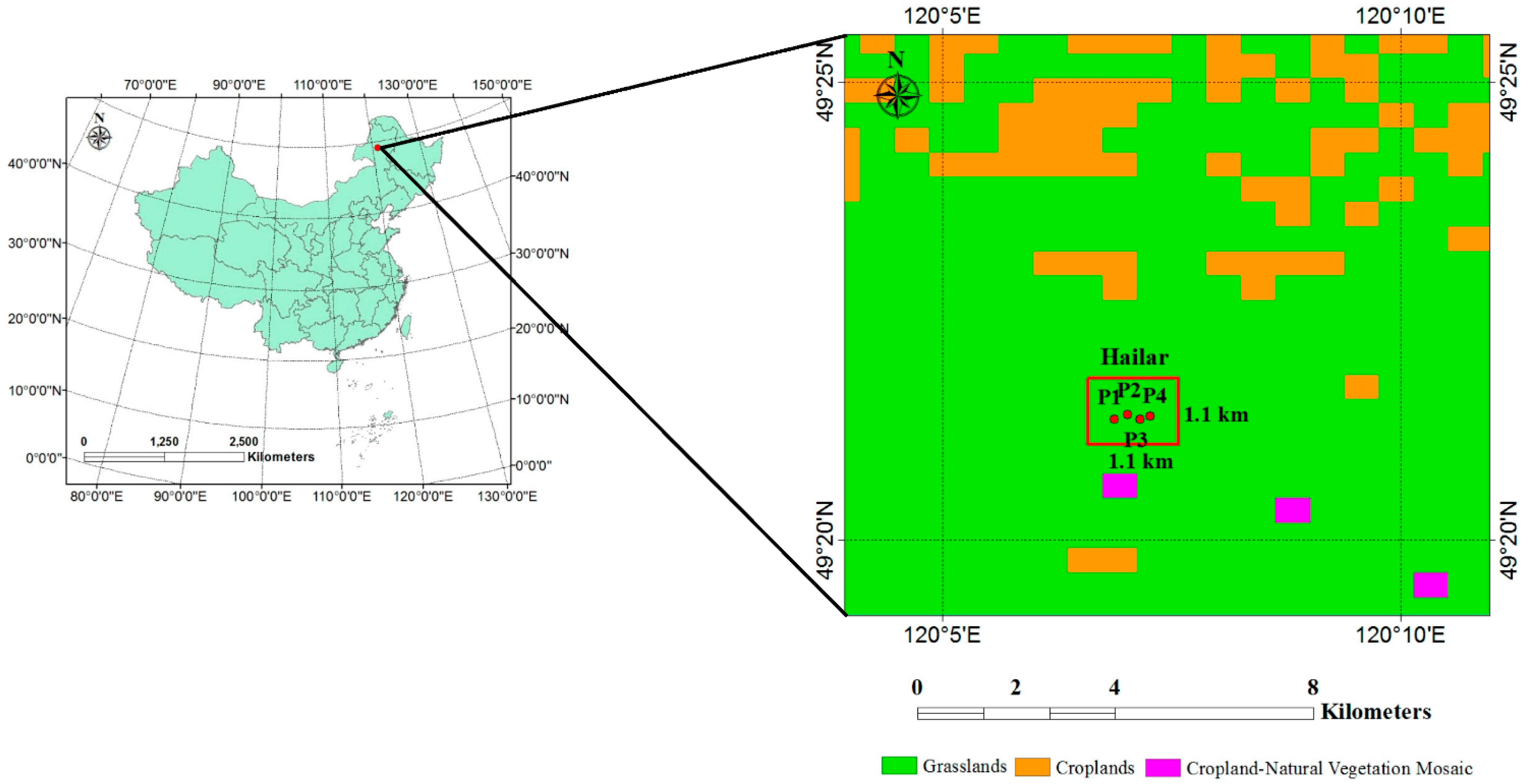
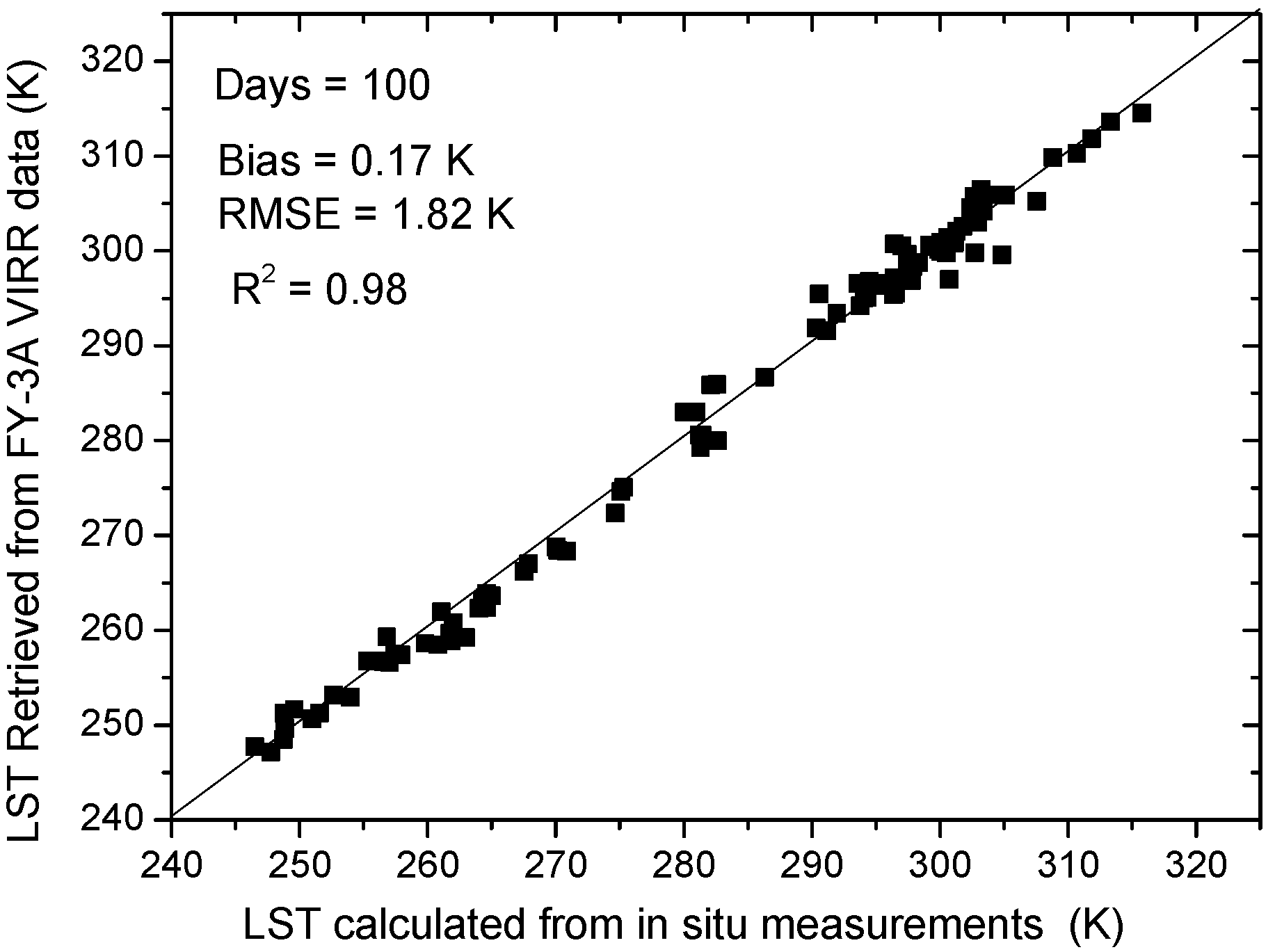
5.3. Validation Using In Situ Measurements

To validate the proposed LST retrieval algorithm, the Hailar field measurements are used. Note that the data measured by the infrared radiometer are ground-based radiances that couple LST, LSE and downwelling atmospheric radiance. The ground-based LST can be retrieved by:
L S T g r o u n d = B λ 1 [ 1 ε λ ( L g r o u n d , λ ( 1 ε λ ) R a t m , λ ) ]
where B 1 is the inversion of the Planck function, L g r o u n d , λ is the radiance emitted from the surface, R a t m , λ is the downwelling radiance from the sky and ε λ is the land surface emissivity.
Because the experimental campaign was conducted over one year from October, 2013, to September, 2014, the land cover of the field site was dry grass from 22 October to 5 November 2013. From 6 November 2013, to 25 March 2014, the site was covered by snow. From April to May, the snow was melting, and the site was again covered by dry grass. From June to September, the land cover at the site was green grass. Consequently, the value of ε λ is assigned a constant 0.940 for dry grass, 0.983 for green grass and 0.988 for snow cover, as calculated by combining the spectral response function of SI-111 with the dry grass spectra, green grass spectra and snow spectra, respectively, provided by the UCSB spectral library database. Figure 12 illustrates the number of days with cloud-free conditions at the time of the FY-3A VIRR overpasses during the experiment period at the Hailar field site.
Figure 12. Number of days with cloud-free conditions at the time of the FY-3A VIRR overpasses during the experimental period at the study site.
Remotesensing 07 03250 g012
Figure 13 provides a comparison between the LSTs retrieved from FY-3A VIRR data using the proposed method and those calculated using Equation (17) from the in situ measurements for all days with cloud-free conditions at the time of the VIRR overpasses. The cloud-free conditions are defined according to the measured ground-based radiance variation, i.e., smooth sinusoidal pattern a half hour before and after the VIRR overpass. The three-minute means of the ground observations were used. This figure shows that the bias and RMSE of the LSTs between two measurements (ground-based and satellite-based methods) are 0.17 K and 1.82 K, respectively. The LSTs estimated using our proposed method are highly correlated with those calculated from in situ measurements, with a squared correlation coefficient (R2) of 0.98. The figure illustrates that the proposed method slightly underestimates the LST for the temperatures between 260 K and 280 K. These cases correspond to the days in October, 2013, and April to May, 2014, when we assume a constant emissivity 0.940 for dry grass; this value may result in a slight overestimation of the LST calculated from the ground-based measurements. In addition, the ground data measured at the site are point-based, while the retrievals with FY-3A VIRR data using our proposed method have a spatial resolution of 1.1 km. The viewing direction of the ground-based radiometers is vertically downward, while the VZAs of the VIRR are variable for each pixel. Consequently, both the spatial scale difference and the viewing angle difference may somewhat affect the comparison of the two resultant LSTs.
Figure 13. Comparison between the LSTs estimated using the proposed method and those calculated using in situ measurements for cloud-free conditions at the time of the FY-3A VIRR overpass during the experiment period at the Hailar site (R2 is the square of the correlation coefficient).
Remotesensing 07 03250 g013

6. Conclusions

In this paper, a split-window algorithm was proposed to retrieve the land surface temperature (LST) from thermal-infrared Channels 4 (centered at 10.8 µm) and 5 (centered at 12.0 µm) of the Visible and Infrared Radiometer (VIRR) onboard the Chinese second-generation polar-orbiting FengYun-3A (FY-3A) meteorological satellite.
On the basis of radiative transfer theory, the proposed split-window algorithm was developed using an accurate atmospheric radiative transfer model, MODTRAN 4, with the latest version of the Thermodynamic Initial Guess Retrieval (TIGR) atmospheric profile database. To improve the accuracy of the split-window algorithm, the LST, the mean emissivity and atmospheric water vapor content (WVC) were divided into several tractable sub-ranges. The simulation analysis showed that the fitting root mean square errors (RMSEs) were proportional to viewing zenith angle (VZA), WVC and LST; the LST could be estimated with RMSEs below 1 K for the VZA sub-ranges less than 30° or for the VZA sub-range less than 60° and the atmospheric WVC sub-range less than 3.5 g/cm2, provided that the LSEs are known.
Sensitivity analyses in terms of the instrument noise and the uncertainty in the LSE and atmospheric WVC were performed. The results showed that, given an instrument noise NEΔT = 0.2 K and 1% uncertainties in ( 1 ε ) and Δε, the total error associated with the LST retrieval was approximately 1.1 K.
Some data that were simulated independently with the same viewing geometry and land surface type conditions, but with different atmospheric conditions, were used to test the performance of the proposed algorithm. Compared with the actual input LSTs, the retrieved results are quite consistent for VZAs with a maximum RMSE of less than 1 K.
The MODIS land surface temperature/emissivity (LST/E) products MOD11_L2 with a 1-km spatial resolution LST were used to inter-validate the proposed algorithm. A comparison of the two satellite-derived LSTs in terms of the geographic coordinate matching, temporal matching and VZA matching showed that the two datasets agree well for homogeneous land surfaces, such as grasses, with an RMSE of 1.68 K. The agreement is poor for heterogeneous land surfaces, particularly barren or sparsely vegetated surfaces, with a RMSE of 3.59 K.
In situ measurements at the Hailar field site in northeastern China from October, 2013, to September, 2014, were used to validate the proposed algorithm. The results showed that the bias and RMSE of the LSTs between the two types of measurements (ground-based and satellite-based methods) were 0.17 K and 1.82 K, respectively.

Acknowledgments

This work was jointly supported by the Excellent Young Talent Funds for Kezhen Distinguished Young Scholar in the Institute of Geographic Sciences and Natural Resources Research (IGSNRR), Chinese Academy of Sciences (CAS) under Grant 2012RC101, the National Natural Science Foundation of China under Grants 41171287 and 41231170 and the “Strategic Priority Research Program” of the Chinese Academy of Sciences, Climate Change: Carbon Budget and Relevant Issues, under Grant XDA05040204.

Author Contributions

Bo-Hui Tang wrote the manuscript and was in charge of the research design, data simulations and data analysis. Zhao-Liang Li conceived of and designed the research. Kun Shao, Hua Wu, Françoise Nerry and Guoqing Zhou collected and analyzed the in situ measurement data and performed the remotely-sensed data processing.

Conflicts of Interest

The authors declare no conflict of interest.

References

  1. Li, Z.-L.; Tang, B.-H.; Wu, H.; Ren, H.; Yan, G.J.; Wan, Z.; Trigo, I.F.; Sobrino, J. Satellite-derived land surface temperature: Current status and perspectives. Remote Sens. Environ. 2013, 131, 14–37. [Google Scholar] [CrossRef]
  2. Li, Z.-L.; Wu, H.; Wang, N.; Qiu, S.; Sobrino, J.A.; Wan, Z.; Tang, B.-H.; Yan, G. Land surface emissivity retrieval from satellite data. Int. J. Remote Sens. 2013, 34, 3084–3127. [Google Scholar] [CrossRef]
  3. Tang, B.-H.; Li, Z.-L. Estimation of instantaneous net surface longwave radiation from MODIS cloud-free data. Remote Sens. Environ. 2008, 112, 3482–3492. [Google Scholar] [CrossRef]
  4. Li, Z.-L.; Tang, R.; Wan, Z.; Bi, Y.; Zhou, C.; Tang, B.-H.; Yan, G.; Zhang, X. A review of current methodologies for regional evapotranspiration estimation from remotely sensed data. Sensors 2009, 9, 3801–3853. [Google Scholar] [CrossRef] [PubMed]
  5. Hansen, J.; Ruedy, R.; Sato, M.; Lo, K. Global surface temperature change. Rev. Geophys. 2010, 48, RG4004. [Google Scholar]
  6. Sobrino, J.A.; Raissouni, N.; Li, Z.-L. A comparative study of land surface emissivity retrieval from NOAA data. Remote Sens. Environ. 2001, 75, 256–266. [Google Scholar] [CrossRef]
  7. Sobrino, J.A.; Jimenez-Munoz, J.C.; Verhoef, W. Canopy directional emissivity: Comparison between models. Remote Sens. Environ. 2005, 99, 304–314. [Google Scholar] [CrossRef]
  8. Becker, F.; Li, Z.-L. Temperature-independent spectral Indices in thermal Infrared bands. Remote Sens. Environ. 1990, 32, 17–33. [Google Scholar] [CrossRef]
  9. Li, Z.-L.; Becker, F. Feasibility of land surface-temperature and emissivity determination from AVHRR data. Remote Sens. Environ. 1993, 43, 67–85. [Google Scholar] [CrossRef]
  10. Wan, Z.; Dozier, J. A generalized split-window algorithm for retrieving land-surface temperature from space. IEEE Trans. Geosci. Remote Sens. 1996, 34, 892–905. [Google Scholar] [CrossRef]
  11. Wan, Z.; Li, Z.-L. A physics-based algorithm for retrieving land-surface emissivity and temperature from EOS/MODIS data. IEEE Trans. Geosci. Remote Sens. 1997, 35, 980–996. [Google Scholar] [CrossRef]
  12. Wan, Z.; Li, Z.-L. Radiance-based validation of the V5 MODIS land-surface temperature product. Int. J. Remote Sens. 2008, 29, 5373–5395. [Google Scholar] [CrossRef]
  13. Gillespie, A.R.; Rokugawa, S.; Matsunaga, T.; Cothern, J.S.; Hook, S.; Kahle, A.B. A temperature and emissivity separation algorithm for Advanced Spaceborne Thermal Emission and Reflection Radiometer (ASTER) images. IEEE Trans. Geosci. Remote Sens. 1998, 36, 1113–1126. [Google Scholar] [CrossRef]
  14. Tang, B.-H.; Bi, Y.; Li, Z.-L.; Xia, J. Generalized Split-Window algorithm for estimate of land surface temperature from Chinese geostationary FengYun meteorological satellite (FY-2C) data. Sensors 2008, 8, 933–951. [Google Scholar] [CrossRef]
  15. Gao, C.; Tang, B.-H.; Wu, H.; Jiang, X.; Li, Z.-L. A generalized split-window algorithm for land surface temperature estimation from MSG-2/SEVIRI data. Int. J. Remote Sens. 2013, 34, 4182–4199. [Google Scholar] [CrossRef]
  16. Jiang, G.-M.; Liu, R. Retrieval of sea and land surface temperature from SVISSR/FY-2C/D/E measurements. IEEE Trans. Geosci. Remote Sens. 2014, 52, 6132–6140. [Google Scholar] [CrossRef]
  17. Wan, Z.; Zhang, Y.; Zhang, Q.; Li, Z.-L. Validation of the land-surface temperature products retrieved from Terra Moderate Resolution Imaging Spectroradiometer data. Remote Sens. Environ. 2002, 83, 163–180. [Google Scholar] [CrossRef]
  18. Hook, S.J.; Vaughan, R.G.; Tonooka, H.; Schladow, S.G. Absolute radiometric in-flight validation of mid infrared and thermal infrared data from ASTER and MODIS on the Terra spacecraft using the lake tahoe, CA/NV, USA, automated validation site. IEEE Trans. Geosci. Remote Sens. 2007, 45, 1798–1807. [Google Scholar] [CrossRef]
  19. Wan, Z. New refinements and validation of the MODIS land-surface temperature/emissivity products. Remote Sens. Environ. 2008, 112, 59–74. [Google Scholar] [CrossRef]
  20. Schneider, P.; Hook, S.J.; Radocinski, R.G.; Corlett, G.K.; Hulley, G.C.; Schladow, S.G.; Steissberg, T.E. Satellite observations indicate rapid warming trend for lakes in California and Nevada. Geophys. Res. Lett. 2009, 36, 1–6. [Google Scholar]
  21. Coll, C.; Caselles, V.; Galve, J.M.; Valor, E.; Niclòs, R.; Sanchez, J.M.; Rivas, R. Ground measurements for the validation of land surface temperatures derived from AATSR and MODIS data. Remote Sens. Environ. 2005, 97, 288–300. [Google Scholar] [CrossRef]
  22. Sobrino, J.A.; Sòria, G.; Prata, A.J. Surface temperature retrieval from Along Track Scanning Radiometer 2 data: Algorithms and validation. J. Geophys. Res. 2004, 109, D11101. [Google Scholar] [CrossRef]
  23. Coll, C.; Valor, E.; Galve, J.M.; Mira, M.; Bisquert, M.; García-Santos, V.; Caselles, E.; Caselles, V. Long-term accuracy assessment of land surface temperatures derived from the Advanced Along-Track Scanning Radiometer. Remote Sens. Environ. 2012, 116, 211–225. [Google Scholar] [CrossRef]
  24. Trigo, I.F.; Monteiro, I.T.; Olesen, F.; Kabsch, E. An assessment of remotely sensed land surface temperature. J. Geophys. Res. 2008, 113, D17108. [Google Scholar] [CrossRef]
  25. Qian, Y.G.; Li, Z.-L.; Nerry, F. Evaluation of land surface temperature and emissivities retrieved from MSG-SEVIRI data with MODIS land surface temperature and emissivity products. Int. J. Remote Sens. 2013, 34, 3140–3152. [Google Scholar] [CrossRef]
  26. Göttsche, F.-M.; Olesen, F.-S.; Bork-Unkelbach, A. Validation of land surface temperature derived from MSG/SEVIRI with in situ measurements at Gobabeb, Namibia. Int. J. Remote Sens. 2013, 34, 3069–3083. [Google Scholar] [CrossRef]
  27. Freitas, S.C.; Trigo, I.F.; Bioucas-Dias, J.M.; Göttsche, F.-M. Quantifying the uncertainty of land surface temperature retrievals from SEVIRI/Meteosat. IEEE Trans. Geosci. Remote Sens. 2010, 48, 523–534. [Google Scholar] [CrossRef]
  28. Guillevic, P.C.; Biard, J.; Hulley, G.C.; Privette, J.L.; Hook, S.J.; Olioso, A.; Göttsche, F.-M.; Radocinski, R.; Román, M.O.; Yu, Y.; et al. Validation of land surface temperature products derived from the Visible Infrared Imager Radiometer Suite (VIIRS) using ground-based and heritage satellite measurements. Remote Sens. Environ. 2014, 154, 19–37. [Google Scholar] [CrossRef]
  29. Li, H.; Sun, D.; Yu, Y.; Wang, H.; Liu, Y.; Liu, Q.; Du, Y.; Wang, H.; Cao, B. Evaluation of the VIIRS and MODIS LST products in an arid area of Northwest China. Remote Sensing of Environment 2014, 142, 111–121. [Google Scholar] [CrossRef]
  30. Barnes, W.L.; Pagano, T.S.; Salomonson, V.V. Prelaunch characteristics of the Moderate Resolution Imaging Spectroradiometer (MODIS) on EOS-AM1. IEEE Trans. Geosci. Remote Sens. 1998, 36, 1088–1100. [Google Scholar] [CrossRef]
  31. Level 1, the Atmosphere Archive and Distribution System (LAADS). Available online: http://ladsweb.nascom.nasa.gov/data/search.html (accessed on 19 March 2015).
  32. NASA-developed EOS Clearinghouse (ECHO). Available online: http://wist.echo.nasa.gov/api (accessed on 19 March 2015).
  33. Snyder, W.C.; Wan, Z.; Zhang, Y.; Feng, Y.Z. Classification-based emissivity for land surface temperature measurement from space. Int. J. Remote Sens. 1998, 19, 2753–2774. [Google Scholar] [CrossRef]
  34. Land Cover Type Yearly L3 Global 500 m SIN Grid. Available online: https://lpdaac.usgs.gov/products/modis_products_table/mcd12q1 (accessed on 19 March 2015).
  35. Sobrino, J.A.; Li, Z.-L.; Stoll, M.P.; Becker, F. Multi-channel and multi-angle algorithms for estimating sea and land surface temperature with ATSR data. Int. J. Remote Sens. 1996, 17, 2089–2114. [Google Scholar] [CrossRef]
  36. Li, Z.-L.; Petitcolin, F.; Zhang, R.H. A physically based algorithm for land surface emissivity retrieval from combined mid-infrared and thermal infrared data. Sci. China Ser. E: Technol. Sci. 2000, 43, 23–33. [Google Scholar] [CrossRef]
  37. McMillin, L.M. Estimation of sea surface temperature from two infrared window measurements with different absorptions. J. Geophys. Res. 1975, 80, 5113–5117. [Google Scholar] [CrossRef]
  38. Becker, F.; Li, Z.-L. Towards a local split window method over land surfaces. Int. J. Remote Sens. 1990, 11, 369–393. [Google Scholar] [CrossRef]
  39. Coll, C.; Caselles, V.; Sobrino, J.A.; Valor, E. On the atmospheric dependence of the split-window equation for land surface temperature. Int. J. Remote Sens. 1994, 15, 105–122. [Google Scholar] [CrossRef]
  40. Berk, A.; Bernstein, L.S.; Anderson, G.P.; Acharya, P.K.; Robertson, D.C.; Chetwynd, J.H.; Adler-Golden, S.M. MODTRAN cloud and multiple scattering upgrades with application to AVIRIS. Remote Sens. Environ. 1998, 65, 367–375. [Google Scholar] [CrossRef]
  41. Thermodynamic Initial Guess Retrieval (TIGR). Available online: http://ara.abct.lmd.polytechnique.fr/index.php?page=tigr (accessed on 19 March 2015).
  42. Platt, C.M.R.; Prata, A.J. Nocturnal effects in the retrieval of land surface temperature from satellite measurements. Remote Sens. Environ. 1993, 45, 127–136. [Google Scholar] [CrossRef]
  43. MODIS UCSB Emissivity Library. Available online: http://www.icess.ucsb.edu/modis/EMIS/html/em.html (accessed on 19 March 2015).
  44. The Johns Hopkins University (JHU) spectral database. Available online: http://speclib.jpl.nasa.gov/ (accessed on 19 March 2015).
  45. Coll, C.; Caselles, V. A split-window algorithm for land surface temperature from advanced very high resolution radiometer data: Validation and algorithm comparison. J. Geophys. Res. 1997, 102, 16697–16713. [Google Scholar] [CrossRef]
  46. Sobrino, J.A.; Raissouni, N. Toward remote sensing methods for land cover dynamic monitoring: Application to Morocco. Int. J. Remote Sens. 2000, 21, 353–366. [Google Scholar] [CrossRef]
  47. Soria, G.; Sobrino, J.A. ENVISAT/AATSR derived land surface temperature over a heterogeneous region. Remote Sens. Environ. 2007, 111, 409–422. [Google Scholar] [CrossRef]
  48. Prata, A.J.; Caselles, V.; Colland, C.; Sobrino, J.A.; Ottle, C. Thermal remote sensing of land surface temperature from satellites: Current status and future prospects. Remote Sens. Rev. 1995, 12, 175–224. [Google Scholar] [CrossRef]
  49. Sobrino, J.A.; Caselles, V.; Coll, C. Theoretical split-window algorithms for determining the actual surface temperature. IL Nuovo Cimento C 1993, 16, 219–236. [Google Scholar] [CrossRef]
  50. Carlson, T.N.; Ripley, D.A. On the relation between NDVI, fractional vegetation cover, and leaf area index. Remote Sens. Environ. 1997, 62, 241–252. [Google Scholar] [CrossRef]
  51. Li, Z.-L.; Jia, L.; Su, Z.; Wan, Z.; Zhang, R. A new approach for retrieving precipitable water from ATSR2 split-window channel data over land area. Int. J. Remote Sens. 2003, 24, 5095–5117. [Google Scholar] [CrossRef]
  52. MODIS Reprojection Tool. Available online: https://lpdaac.usgs.gov/tools/modis_reprojection_tool (accessed on 19 March 2015).

