Article

Global and Local Real-Time Anomaly Detectors for Hyperspectral Remote Sensing Imagery

1
College of Information and Communication Engineering, Harbin Engineering University, Harbin 150001, China
2
College of Computer Science and Technology, Harbin Engineering University, Harbin 150001, China
*
Authors to whom correspondence should be addressed.
Remote Sens. 2015, 7(4), 3966-3985; https://doi.org/10.3390/rs70403966
Submission received: 23 October 2014 / Revised: 18 March 2015 / Accepted: 18 March 2015 / Published: 1 April 2015

Abstract

:
Anomaly detection has received considerable interest for hyperspectral data exploitation due to its high spectral resolution. A well-known algorithm for hyperspectral anomaly detection is the RX detector. A number of variations have been studied since then, including global and local versions for different type of anomalies. Aiming at a real-time requirement for practical applications, this paper extends the concept of global and local anomaly detectors to be real-time detectors. The algorithms exploit the fact that a true real-time detector must produce its output in a causal manner and at the same time as an input comes in. Taking advantage of the Woodbury matrix identity, the global and local real-time detectors can be implemented and processed pixel-by-pixel in real time. Both synthetic and real hyperspectral imagery are conducted to demonstrate their performance.

Graphical Abstract

1. Introduction

Hyperspectral imagery (HSI) processing methodology has generally become increasingly important due to its very high spectral resolution and capability of uncovering many subtle materials that cannot be known by traditional remote sensing monitors. Anomaly detection (AD) is very important for practical use since, in most applications, no prior knowledge of the target spectrum or background information is available before the process of detection—for example, special species in agriculture and ecology, rare minerals in geology, toxic wastes in environmental monitoring, oil spills in water pollution, drug trafficking and smuggling in law enforcement, man-made objects in battlefields, unusual terrorism activities in intelligence gatherings, tumors in medical imaging, etc. [1,2]. Since no prior knowledge is assumed, the detection is typically based on a statistical characterization of the multivariate data. Those pixels with significantly different spectral signatures from their neighboring background pixels or the global background pixels are detected as anomalies.
Many types of anomaly detectors have been proposed in the literature [3,4,5,6,7,8,9,10,11,12,13,14,15,16]. They fall into two categories, global and local methodologies. In global AD algorithms, small rare targets with significantly different spectral signatures from global spectral statistics are defined as anomalies. The most popular global AD algorithm, developed by Reed and Xiaoli Yu, refers to an RX detector [4], which is considered the benchmark AD approach for multi- and hyperspectral imagery. Basically, an RX detector is a constant false alarm rate (CFAR) detector derived by the generalized likelihood ratio test (GLRT). It actually performs a Mahalanobis Distance calculation between the pixel being processed and the background information. In [6], Kwon presents a nonlinear model of RX detector, called Kernel RX. The Kernel RX detector achieves a better performance by mapping the original input space to a higher-dimensional space via a non-linear function, especially when the original signatures are mixed in a non-linear model, which is always the case in reality. Thanks to the “kernel-trick” [17], the Kernel RX detector could be implemented in the higher-dimensional space by means of kernel functions defined on pairs of dot products of input data, without identifying the non-linear mapping function. Chang presents many other global AD algorithms, including Low Probability Detection (LPD) [18], Constrained Energy Minimization (CEM) [19,20], etc. Unlike the RX detector, the LPD algorithm uses unity vector with ones in all the components as its match signal, while RX uses the pixel being processed. CEM, on the other hand, is a target detection algorithm that could detect small and sub-pixel targets of interest in the hyperspectral imagery. The target signature could be obtained in advance by endmember extraction algorithms or other pre-processing techniques.
Local AD algorithms, on the other hand, are of importance due to the weakness of global AD algorithms when the targets are extremely small or only abnormal in a local background but buried in the global background. The local AD algorithms are designed to detect pixels whose spectral signatures are conspicuous or inconspicuous in relation to surrounding pixels. Variants of local AD algorithms consist of applying locally the same concept of a sliding window centered by the pixel under test, of which the most popular is the local RX detector derived from the benchmark RX detector [12,13,14]. There are also many other local AD algorithms in the literature; for example, Kwon et al. recently developed the so-called dual window-based eigenspace separation transform (DWEST) [15]. An alternative approach, called nested spatial window-based target detection (NSWTD), uses a set of nested spatial windows to detect anomalies [21,22].
Despite the fact that many global and local AD algorithms have been proposed in the literature, most of them are time-consuming and difficult for hardware implementation due to the large amount of computing power needed for matrix and matrix inversion. However, in practical applications, there is an increasing interest in real-time processing for hyperspectral imagery. Several attributes may enhance the need for real-time anomaly detection for hyperspectral imagery. One may be that finding some targets, especially moving targets, quickly is essential in decision-making. The other reason may be that, with the development of modern remote sensing technology, hyperspectral imagery can offer more detailed information; at the same time, it also has challenges of data storage, transmission, and system responding time due to the huge amount of hyperspectral data. With a real-time processing algorithm, we could reap the benefits of reducing data storage, which is important in data processing and getting pre-AD results in the course of data transmission. Despite the fact that there are many so-called real-time anomaly detection algorithms in the literature [23,24,25,26,27], to the authors’ best knowledge, almost none of them are actual real-time procedures but simply fast algorithms. In order to address the real-time issue in hyperspectral anomaly detection, this paper presents pixel-by-pixel real-time processing algorithms for both global and local AD in hyperspectral imagery. Both synthetic and real hyperspectral imagery experiments are designed to show the real-time procedure and the difference between global and local real-time detectors.
This paper is organized as follows. Section 2 describes the methodologies of commonly used global and local anomaly detectors. Section 3 presents the real-time anomaly detection algorithms for both global and local forms. In Section 4 synthetic data and real hyperspectral imagery are conducted using all the AD algorithms above, including non-real-time and real-time versions, to prove the efficiency of the proposed methods. Finally, some conclusions are drawn in Section 5.

2. Commonly Used Global and Local Anomaly Detectors

The most widely used anomaly detector is probably the one developed by Reed and Xiaoli Yu in [4], referred to as K-RX detector (K-RXD), where K is the global sample covariance matrix. Since then many versions of RX-type anomaly detectors have been proposed including a correlation-matrix-based RX detector and some local detectors using a sliding window to make anomaly detection adaptive [6,8,12,13,14].

2.1. Global RX Detector

Reed and Yu [4] developed, through a GLRT, a so-called RX anomaly detector for HSI data, assuming that the spectrum of the received signals (spectral pixels) and the covariance of the background clutter are unknown. It attempts to locate anything that looks different from the entire background clutter. Let each input spectral signal consisting of L spectral bands be denoted by xi = [x1i, x2i, …, xLi]. The two competing hypotheses that the RX algorithm needs to distinguish are given by:
{ H 0 : x = n ( target absent ) H 1 : x = a s + n ( target present )
where a = 0 under H0 and a > 0 under H1, respectively. n is a vector that represents the background clutter noise process, and s is the spectral signature of the signal (target) given by s = [s1, s1, …, sL,]T. The target signature and background covariance are assumed to be unknown. The model assumes that the data arise from two normal probability density functions with the same covariance matrix but different means. Under H0 (background clutter), the data is modeled as N (0, Cb), and under H1 the data is modeled as N (s, Cb).
Assuming a single pixel target as the observation test vector r, the RX detector (RXD), referred to as δRXD(r), is specified by:
δ RXD ( r ) = ( r μ ) T K 1 ( r μ ) > η
where μ is the estimated background sample mean, K is the background covariance matrix estimated from the background pixels, and η is the threshold. It should be pointed out that the model assumes the data arise from two normal probability density functions with the same covariance matrix but different means.
The form of δRXD(r) in Equation (2) is actually the well-known Mahalanobis distance. Since K is a non-negative definite matrix it can be expressed as K = K1/2K1/2. Using K1/2 as a transform matrix, Equation (2) can be simply reduced to:
δ RXD ( r ) = ( r μ ) T K 1 / 2 K 1 / 2 ( r μ )   = ( K 1 / 2 r K 1 / 2 μ ) T ( K 1 / 2 r K 1 / 2 μ )   = r ˜ T r ˜ = r ˜ 2
with r ˜   = K−1/2 (rμ) Equation (3) shows that RXD actually calculates r ˜   , the square of the vector length of r ˜   , which represents the gray-level intensity of r ˜   . So, from a detection point of view, K−1/2 can be interpreted as a whitening matrix. However, from a signal processing point of view, using K and μ to remove the first two order statistics is called data sphering. Since the image background can be generally described by the 2nd order statistics, RXD performs anomaly detection by finding the higher intensities of sphered data sample vectors. In other words, anomaly detection is enhanced by anomaly contrast resulting from removing image background via data sphering in Equation (3) so as to achieve background suppression.
Chang replaces global covariance in Equation (2) with a sample correlation matrix, referred to as R-RX detector (R-RXD) [18], specified as follows:
δ R - RXD ( r ) = r T R 1 r
where R is the global sample data autocorrelation matrix formed by R =   ( 1 / N ) i = 1 N r i r i T .
The form of RXD in Equation (1) may not explain quite how an anomaly detector performs by using its detected intensity and contrast. However, by virtue of Equation (4), the concept of intensity and contrast in anomaly detection algorithms can be explained well by R-RXD. First of all, the form of Equation (4) can be decomposed into two components, R1r and rT. The first component, R1r, carried out by R-RXD, actually performs background suppression via the use of global sample correlation matrix to increase the contrast of anomalies against the entire image background. This is followed by the second component, rT, which uses a matched filter to detect the intensity of anomalies via matching the background-compressed data sample R1r, using its own signature r as a matched signal source vector. Since such a matched filter takes an inner product of the incoming signal source vector r with the matched signal source vector R1r, it actually performs the spectral angle mapping (SAM) by calculating the angle between R1r and rT.
Following the same argument, Equation (1) can also be interpreted in a similar way, except that the data sample r is now replaced by rμ and the global correlation matrix R is replaced by the covariance matrix K. However, it should be noted that this is a significant difference between R-RXD and original covariance-based RXD because the former detects the data sample vector itself while the latter actually detects the data sample variation from the global sample mean, i.e., data sample vectors that have large gradients. So, technically speaking, the original covariance-based RXD does not detect intensities of anomalies themselves but rather their gradient intensities. As a result, RXD works as a distance measure like Mahalanobis distance, while R-RXD can be considered as a matched filter.

2.2. Local RX Detector

Local anomaly detection is very important since the global RX anomaly detector fails to work when the anomalies are relatively small or only distinct from the local surroundings but buried in the global background. The most widely used local anomaly detection algorithm, derived from the commonly used RXD, is the local-RX detector (LRXD), which makes use of a local dual window to get the local background statistics sliding through the whole data set. The form of the dual window is shown in Figure 1. Sliding dual window for LRXD, which is the commonly used local sliding window for hyperspectral anomaly detection.
Figure 1. The sliding dual window for LRXD is the most commonly used for hyperspectral anomaly detection.
Remotesensing 07 03966 g001
The LRXD is specified as follows:
δ LRXD ( r ) = ( r μ l o c a l ) T K l o c a l 1 ( r μ l o c a l )
where μlocal is the local background mean and Klocal is the local background covariance matrix.
This local anomaly detection returns a higher detection rate due to the fact that the local background model can be tightly fitted. However, this is accompanied by a proper window size, which is unknown, and the problem is there is no universal way to completely avoid over-fitting or under-fitting. Another problem is that this process is time-consuming. The LRXD detector is computationally more expensive than the original RXD, caused by a repeated calculation of a covariance/correlation matrix and its inverse in every local window as opposed to the global RXD, which performs only once for the entire data set.

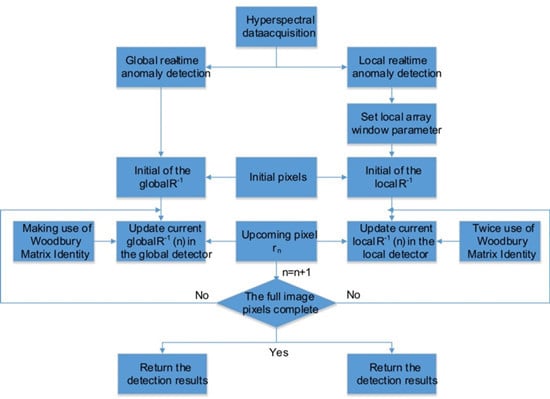
3. Real-Time Anomaly Detectors

None of the global and local RX detectors mentioned above are actually real-time detectors since they need to use either the entire data vectors or the data vectors in the local window, which also include future pixels. Once the causal version specified by Equation (4) is proposed, a follow-up task is to implement it pixel-by-pixel in a real-time way so as to achieve real-time processing. The following Woodbury matrix identity [28,29] is very helpful:
[ A + u v T ] 1 = A 1 [ A 1 u ] [ v T A 1 ] 1 + v T A 1 u

3.1. Global Real-Time Detector

In order to implement the real-time RX detector, a causal version of the RX detector (CRXD) is firstly introduced here. Let { r i } i = 1 N (N is the total number of pixels of the entire data set) be a set of data sample vectors to be processed. The causal RX detector (RXD) [30], denoted by δCRXD(rn), is specified by:
δ CRXD ( r n ) = r n T R ( n ) 1 r n
where rn is the nth data sample vector currently being processed, R(n) is the sample autocorrelation matrix formed by R ( n ) =   ( 1 / n ) i = 1 n r i r i T , and ri = (ri1, ri2, …, riL,)T is the ith data sample vector (where L is the total number of spectral bands).
Since the causal sample autocorrelation matrix is defined by R ( n ) =   ( 1 / n ) i = 1 n r i r i T , R−1(n) can be re-expressed as follows:
R 1 ( n ) = [ 1 n i = 1 n r i r i T ] 1 = n [ i = 1 n r i r i T ] 1   = n [ ( n 1 ) 1 n 1 i = 1 n 1 r i r i T + r n r n T ] 1   = n [ ( n 1 ) R ( n 1 ) + r n r n T ] 1
Now, by virtue of Equation (6) we can get a global real-time causal R-RXD (GRTCR-RXD), and the inverse of the correlation matrix can be obtained by a causal innovations information update equation where the R−1(n) can be easily updated by R−1(n − 1) as well as the current input data sample vector rn. If we follow Equation (8) and use Equation (6) by letting A = (n − 1)R(n − 1) and u = v = rn, then we will have Equation (9):
R 1 ( n ) = n [ ( n 1 ) R ( n 1 ) + r n r n T ] 1   = n { 1 n 1 R ( n 1 ) 1 [ 1 / ( n 1 ) R ( n 1 ) 1 r n ] [ 1 / ( n 1 ) r n T R ( n 1 ) 1 ] 1 + 1 / ( n 1 ) r n T R ( n 1 ) 1 r n }   = n n 1 R ( n 1 ) 1 n R ( n 1 ) 1 r n r n T R ( n 1 ) 1 ( n 1 ) 2 + ( n 1 ) r n T R ( n 1 ) 1 r n
Then R−1(n) can be expressed as Equation (9) and the final GRTCRXD is specified in Equation (10), where δ ˜ =   r n T R ( n 1 ) 1 r n and M =   r n T R ( n 1 ) 1 :
δ GRTCRXD ( r n ) = r n T R 1 ( n ) r n = n n 1 δ ˜ n δ ˜ Μ ( n 1 ) 2 + ( n 1 ) δ ˜

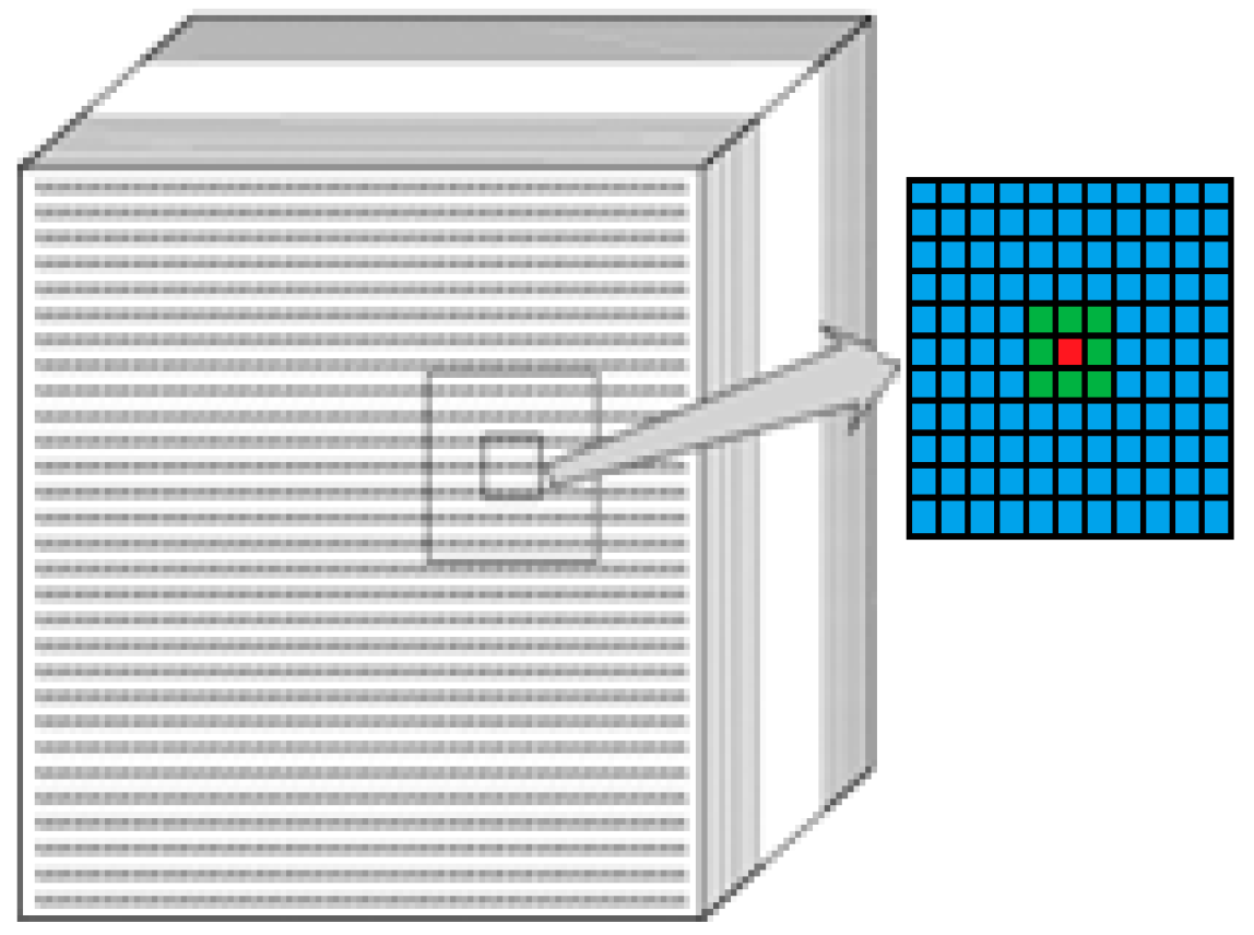
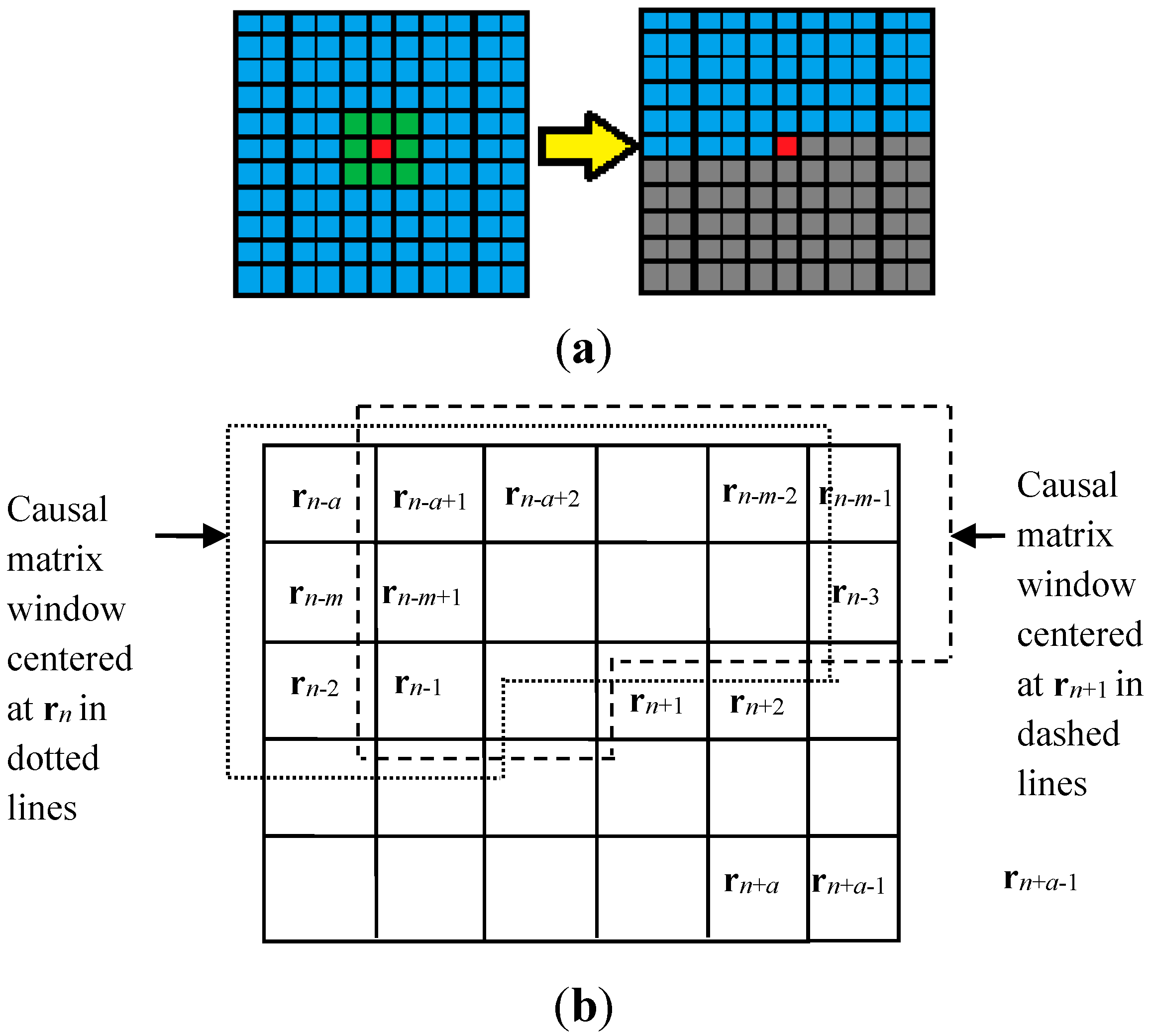
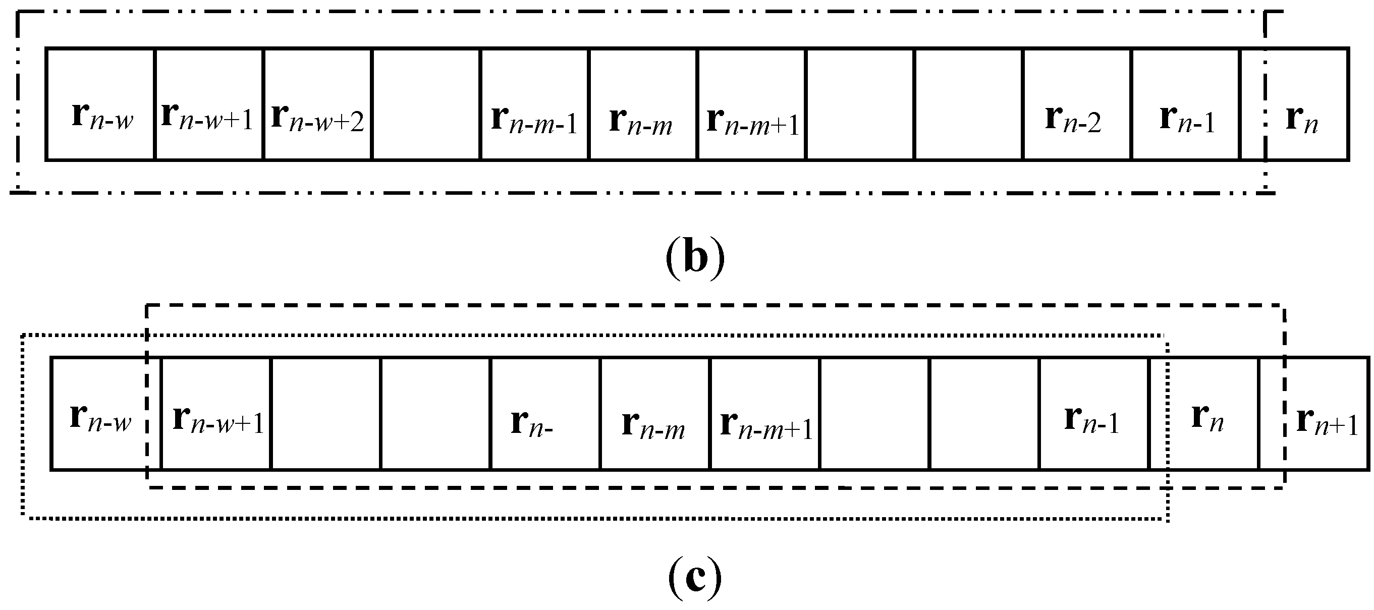
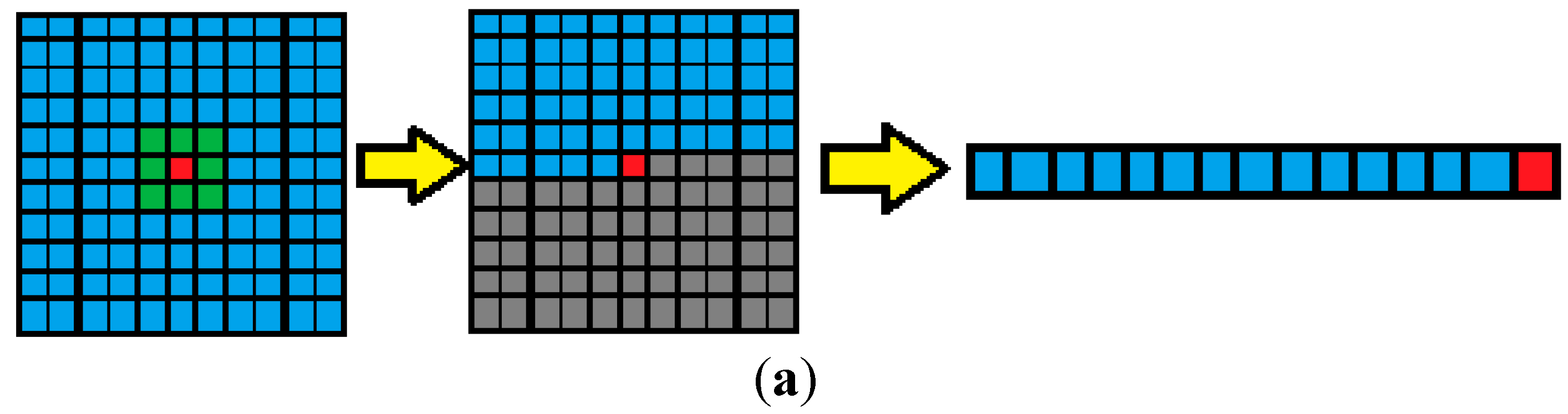
3.2. Local Real-Time Detector

The local anomaly detector is of particular importance, as we have explained in Section 2. However, there are still some weaknesses, of which the most severe is that all the local AD algorithms are time-consuming and computationally more expensive than the original global RX, caused by a repeated calculation of a covariance/correlation matrix and its inversion in every local window. Most real-time detectors are implemented in a global view; there is no real-time anomaly detection algorithm in the form of a local view. Local real-time detection is more difficult to implement than the global version. One of the reasons may be that the sliding window in the commonly used local AD algorithms still needs future pixels after the pixel being processed, as shown in Figure 1. If we want to let the local anomaly detector to work in to a truly real-time manner, we must design a causal sliding window in which background pixels only include the pixels before, that is to say, no further pixels should be included in the local causal window. It is much more difficult to get the inversion of a correlation matrix in a recursive manner since more than one pixel in the local window will change each time. The correlation matrix R(n) is no longer an easy addition function of R(n − 1) but must include the new information rn we derived in Equation (9) for the global real-time detector.
In order to solve the first problem, a Causal Matrix (CM) local window is firstly presented, as shown in Figure 2.
Figure 2. (a) Causal matrix local window derived from the traditional local window; (b) Causal matrix local windows at rn and rn+1.
Remotesensing 07 03966 g002
This CM local window comes from the view of the traditional local window and the concept of “causal” characteristics, i.e., that the detector could only use those pixels prior to the pixel currently being processed; no further information could be included. It is a little bit different from the traditional local window, which is formed by an inner window and an outer window centered by the pixel to be processed. The pixels in blue are background information in Figure 2a, removing all the further pixels in gray color. Figure 2b shows how the causal matrix window slides and how information changes caused by in-and-out pixels. When the window slides from rn (dotted line window) to rn+1 (dashed line window), all the far left column pixels in the dotted line window are going out and all the far right column pixels in the dashed line window need to be added.
The local real-time detector based on CM window is specified as follows:
δ LRTCMRXD ( r n ) = r n T R ˜ ( n ) 1 r n
Technically speaking, Equation (11) can be implemented in real time. However, with a complex, real-time AD algorithm, using the CM window is no longer as easy as the global real-time detector, in which only one recursive equation is able to update R−1(n) for detection. As we can see from Figure 2b, all data sample vectors excluded from the causal matrix window are not removed in sequence. For example, in Figure 2b the rna, rnm, and rn−2 in the causal matrix window centered at rn are removed from the causal matrix window centered at rn+1, while rnm−1 and rn−3, which are not included in the causal matrix window centered at rn, are now added to the causal matrix window centered at rn+1. Obviously, it requires a bookmark to keep track of which data sample vectors should be removed and which data sample vectors should be added as a causal matrix window moves on. Otherwise, the CM window may need to follow the same method as LRXD—loading and storing all pixels in the local window, then calculating R (n) and R−1(n) repeatedly while the window slides. This processing does not meet the real-time requirement since it is time-consuming, even though the processing procedure has already been causally identified.
In order to resolve this issue, we can stretch out the causal matrix window in Figure 2b as a linear array shown in Figure 3. By virtue of Figure 3a, we define a causal array window of width w sliding along with a processed data sample vector rn as a linear array { r i } i = n w n 1 , shown in Figure 3b, named a causal array (CA) local window.
Thus, a CA window moves along with the process of the image data, it simply performs like a queue, first in and first out. In fact, the CA local window is no longer the traditional matrix window of a square window, as shown in Figure 1, but a linear array window consisting of w data sample vectors preceding the current processed data sample rn. The In order to make it clear how the CA local window works, Figure 3c shows the CA window at rn (depicted by dotted lines) and at rn+1 (depicted by dashed lines), where the farthest data sample vector rnw from rn in the causal array window at rn is removed from the causal array window at rn+1, while the most recent data sample vector rn is then added to the causal array window at rn+1.
In order to resolve the processing time issue, a recursive causal information update equation is derived using the same methodology as the global real-time AD algorithm, the Woodbury matrix identity. However, there is a small difference, in that the local real-time AD algorithm needs to apply the Woodbury matrix identity twice in order to get the update equation. The detector formula is the same as LRTCMRXD, marked as LRTCARXD:
δ LRTCARXD ( r n ) = r n T R ˜ ( n ) 1 r n
Figure 3. (a) Three different local windows; (b) causal array window of width w; (c) causal array local windows at rn and rn+1.
Remotesensing 07 03966 g003aRemotesensing 07 03966 g003b
Assume that the width of a sliding causal array window is w and the data sample vector to be processed is rn. To emphasize the width of w and the processed data sample vector rn, we rewrite R ˜ ( n ) in Equation (12) as R ˜ w ( n ) . Then according to Figure 3c, R ˜ w ( n + 1 ) can be further expressed as:
R ˜ w ( n + 1 ) = 1 w i c u r r e n t w i n d o w r i r i T = 1 w [ i p r e v i o u s w i n d o w r i r i T r n w r n w T + r n r n T ]   = R ˜ w ( n ) 1 w r n w r n w T + 1 w r n r n T
Assuming the first two parts, as a whole, equate to
R ˜ ˜ w ( n ) = R ˜ w ( n ) 1 w r n w r n w T
Then, according to Equation (13) and (14), we would have
R ˜ w ( n + 1 ) = R ˜ ˜ w ( n ) + 1 w r n r n T
Then we apply the first use of the Woodbury identity in Equation (6) by letting A = R ˜ ˜ w ( n ) and u = v = 1 / w   r n . Thus R ˜ w 1 ( n + 1 ) can be expressed as Equation (16):
R ˜ w 1 ( n + 1 ) = [ R ˜ ˜ w ( n ) + 1 w r n r n T ] 1   = R ˜ ˜ w 1 ( n ) ( 1 / w ) R ˜ ˜ w 1 ( n ) r n r n T R ˜ ˜ w 1 ( n ) 1 + ( 1 / w ) r n T R ˜ ˜ w 1 ( n ) r n
Now, in order to calculate the inverse of R ˜ w ( n + 1 ) , i.e., R ˜ w 1 ( n + 1 ) , we need to get the innovation information R ˜ ˜ w 1 ( n ) first, where the second use of the Woodbury matrix identity is applied. The Woodbury matrix identity used here could be specified as:
[ A u v T ] 1 = A 1 + [ A 1 u ] [ v T A 1 ] 1 v T A 1 u
Referring to Equations (14) and (17), we could get R ˜ w 1 ( n ) by letting A = R ˜ w ( n ) and u = v = 1 / w   r n w , shown as follows:
R ˜ ˜ w 1 ( n ) = [ R ˜ w ( n ) 1 w r n w r n w T ] 1   = R ˜ w 1 ( n ) + ( 1 / w ) R ˜ w 1 ( n ) r n w r n w T R ˜ w 1 ( n ) 1 ( 1 / w ) r n w T R ˜ w 1 ( n ) r n w
By virtue of Equation (16) and (18), R ˜ w ( n + 1 ) can be updated recursively by R ˜ w ( n ) via deleting the information rnw and adding the new information rn, so as to realize the real-time procedure of the local anomaly detection in Equation (12).

4. Experiments

In this section, three sets of hyperspectral data, including two synthetic images and one real image, are used for global and local real-time implementations.

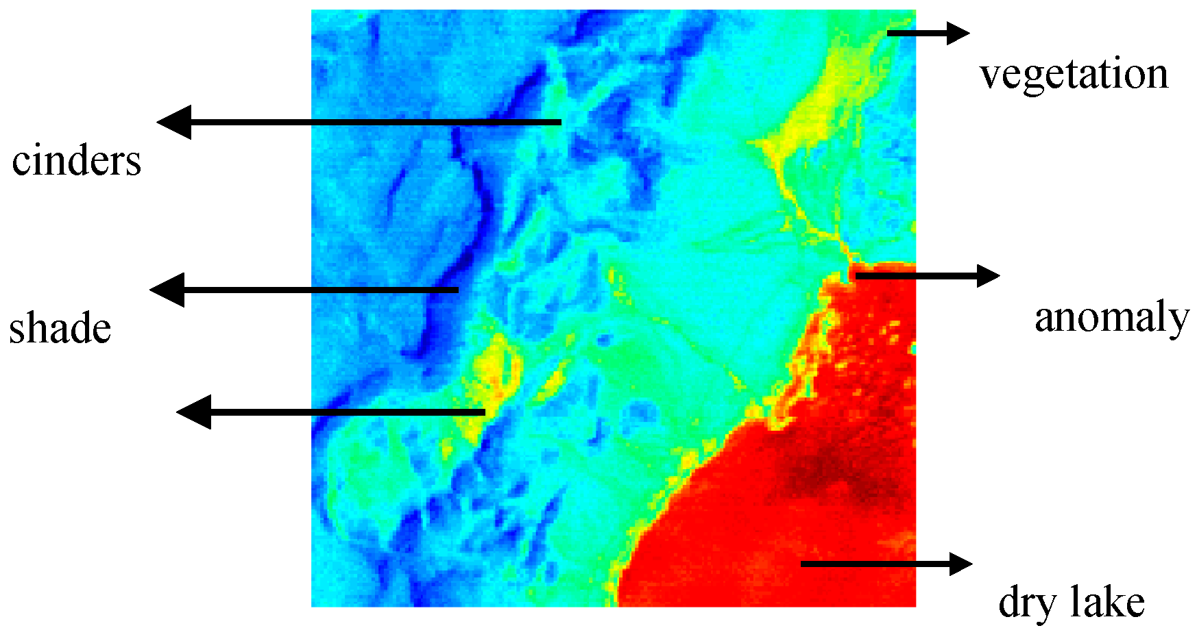
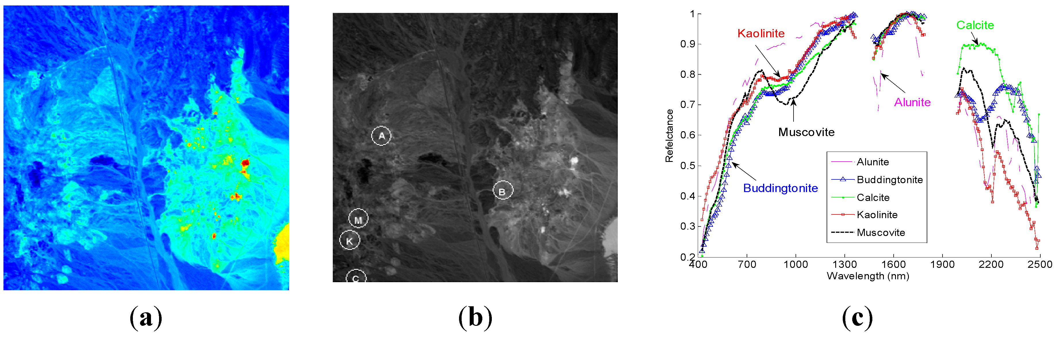
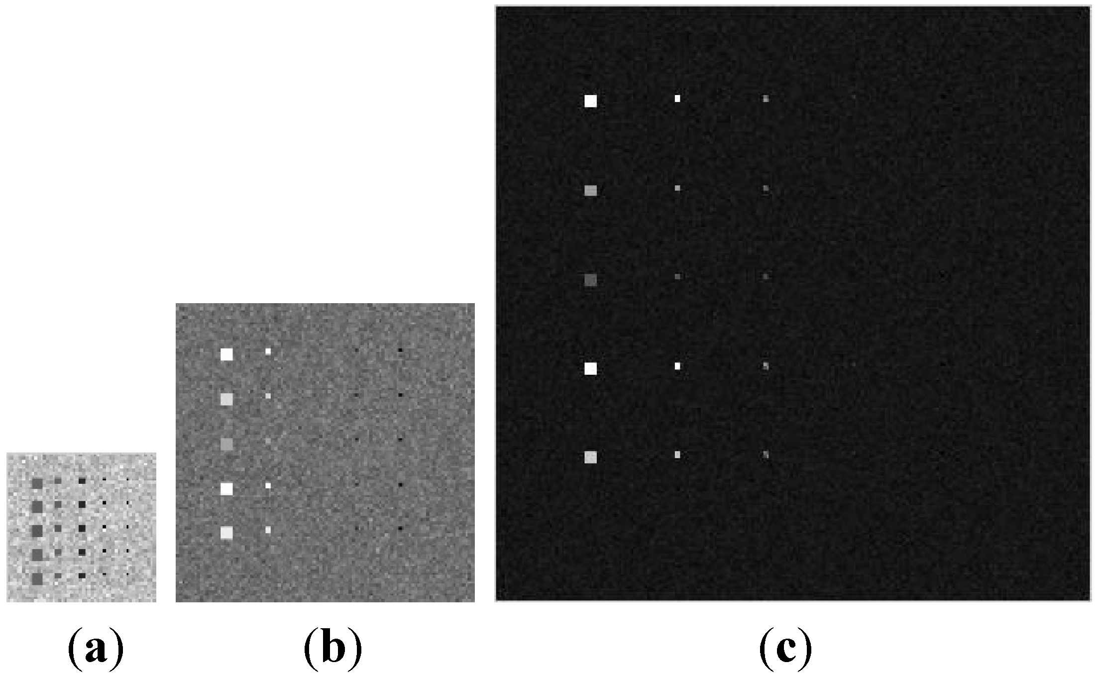
4.1. Data Set Descriptions

In order to verify the performance of proposed real-time detectors, both synthetic and real hyperspectral datasets are used to evaluate our methods.
A synthetic hyperspectral data is custom designed with real ground truth for analysis. The synthetic images are simulated by a real Cuprite image scene with 189 bands, as shown in Figure 4a, which is available at the USGS website [31]. The ground truth available for this region provides the pixel locations of five minerals: alunite (A), buddingtonite (B), calcite (C), kaolinite (K), and muscovite (M), shown in Figure 4b. The spectral features of the five pure minerals are shown in Figure 4c.
Figure 4. (a) Cuprite AVIRIS image scene; (b) spatial positions of A, B, C, K, and M; (c) spectra of the five signatures extracted from the scene in (b).
Remotesensing 07 03966 g004
The synthetic images are designed especially in terms of local detectors, compensating for the weakness of global AD algorithms when the targets are extremely small or only abnormal in a local background but buried in the global background. The five mineral spectral signatures—A, B, C, K, M, marked by circles in Figure 4b—are used to simulate 25 panels with different sizes in Figure 5a. Figure 5b gives the 100th band of the synthetic hyperspectral image.
Another type of hyperspectral image data to be used for experiments is a real AVIRIS image scene, shown in Figure 6, which is the Lunar Crater Volcanic Field (LCVF) with the parameters shown in Table 1.
Figure 5. (a) A set of 25 simulated panels; (b) 100th band of synthetic hyperspectral image.
Remotesensing 07 03966 g005
Figure 6. AVIRIS LCVF subscene.
Remotesensing 07 03966 g006
Table 1. Parameters of AVIRIS LCVF.
SensorAVIRIS
Wavelength400–1800 nm
Bands158
Spectral resolution10 nm
Spatial resolution20 m
Image size200 × 200
Gray range0–10,000
LocationNorthern Nye County, NV

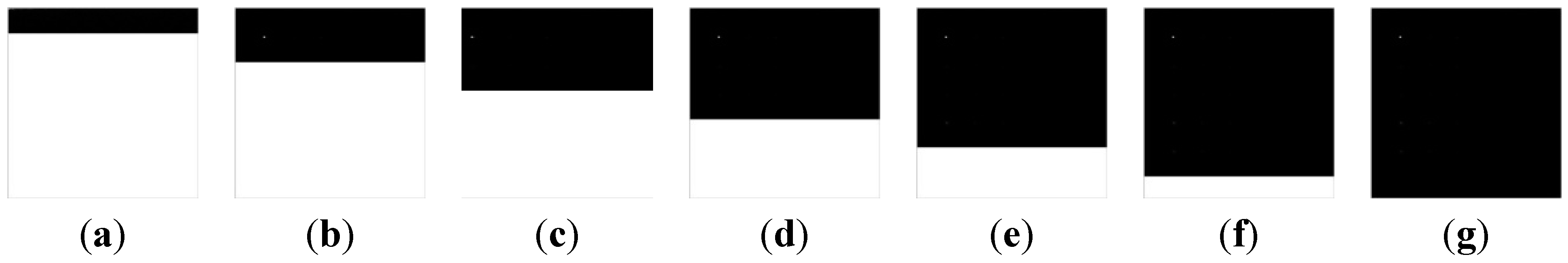
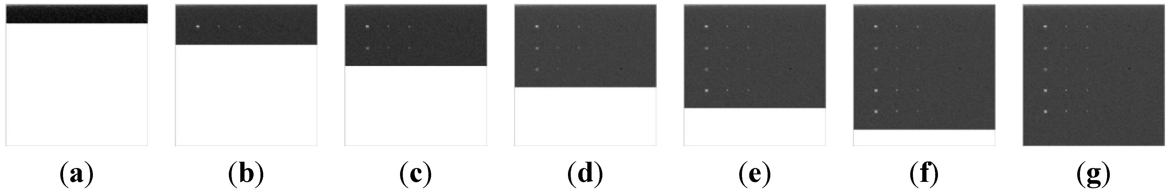
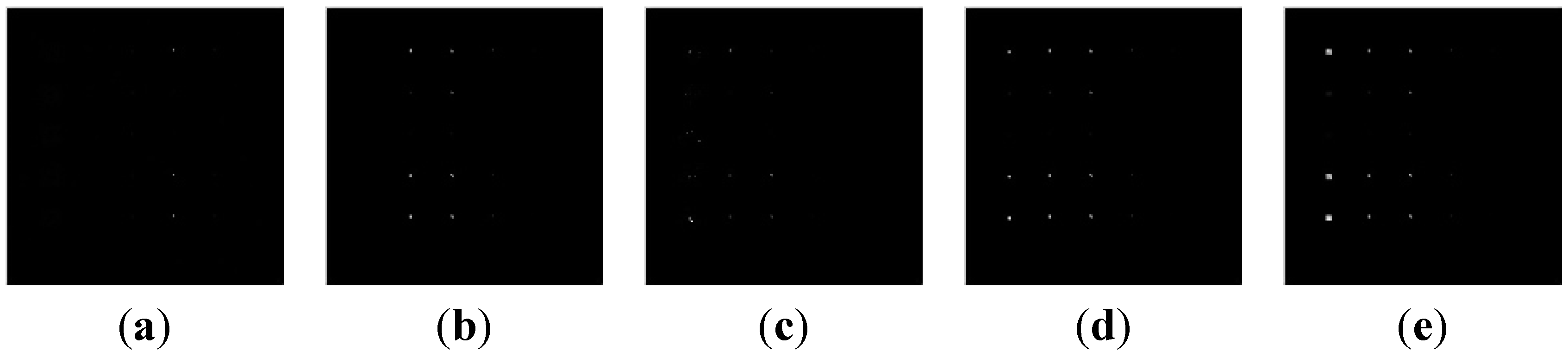
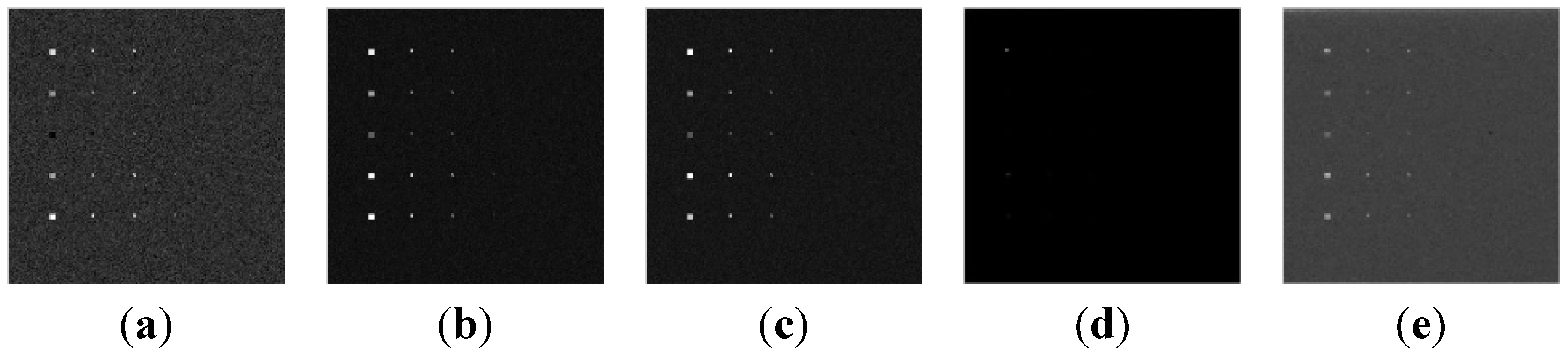
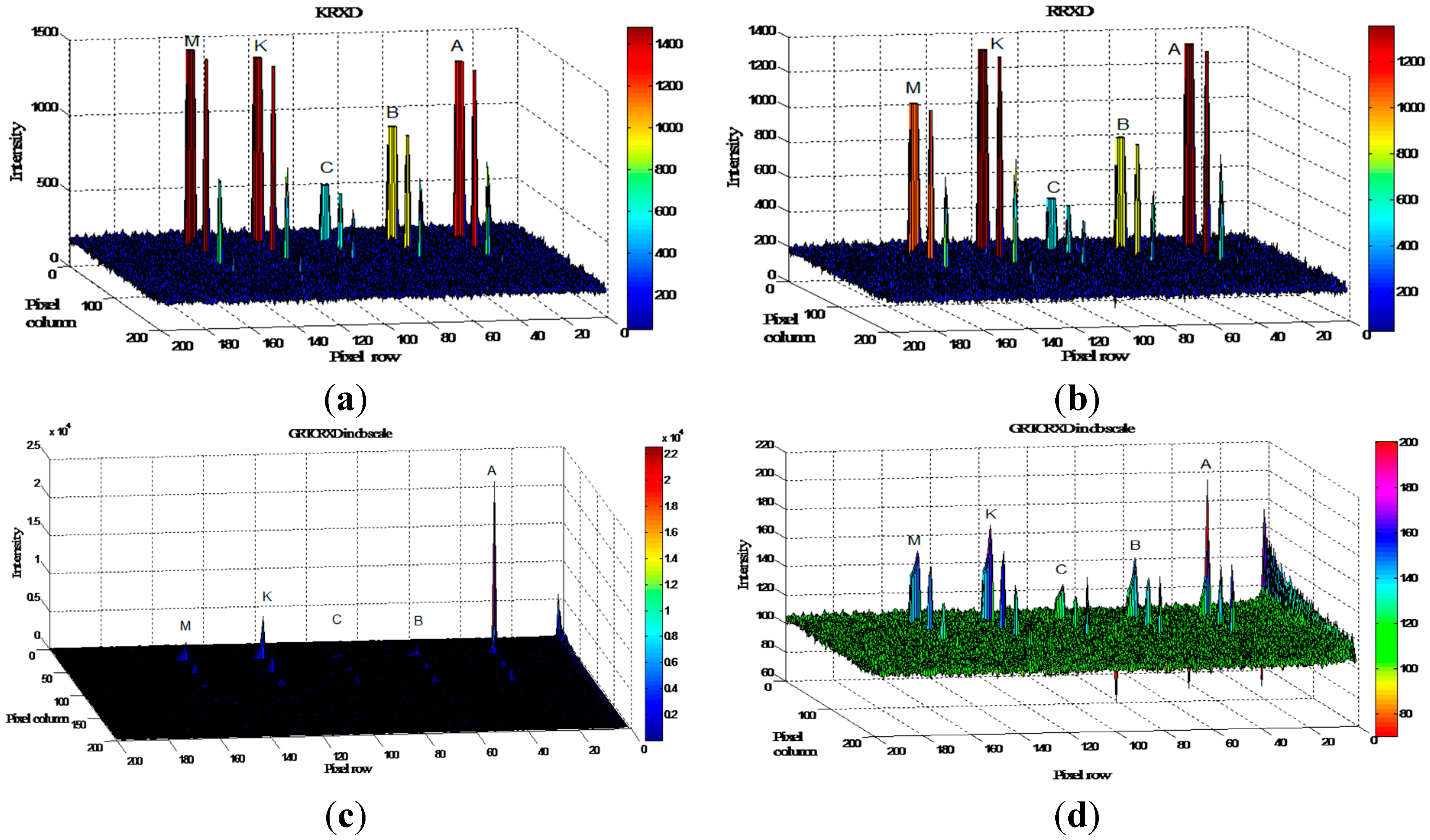
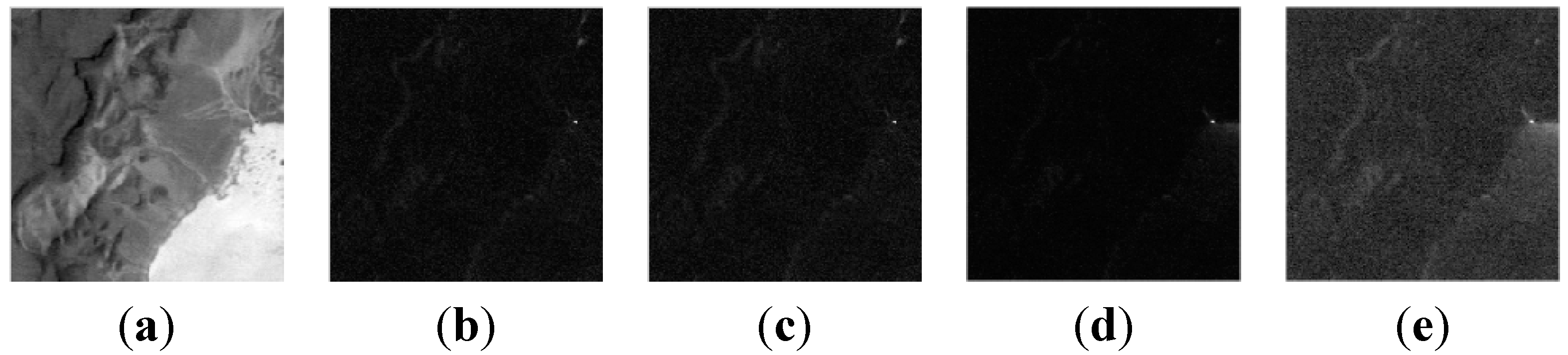
4.2. Global Real-Time Processing Experiments

Several issues arising in anomaly detection have been discussed. One question of particular interest is “what is an anomaly?” In other words, what types of targets are considered as anomalies? A first attempt to address this issue was made in [32], which concluded that an anomaly is closely related to its size relative to the image to be processed.
In this section, before conducting the global real-time processing experiments, the following simple example provides a clue to how controversial this issue is. Figure 7a–c shows the same set of target panels given above with image sizes of 50 × 50 pixel vectors, 100 × 100 pixel vectors and 200 × 200 pixel vectors, respectively. All of the targets are clearly detected in Figure 7a with an image size of 50 × 50; however, the 2 × 2 mixed-pixel panels in the third column are missing in the 100 × 100 image in Figure 7b and all the 1 × 1 sub-pixel panels are missing from the 200 × 200 image in Figure 7c. The experimental results give further evidence that an anomaly is closely related in size to the image to be processed.
Several experiments are then implemented on both synthetic and real hyperspectral images to verify the effectiveness of the global real-time processing. The 100th band of the synthetic data is shown in Figure 8a. We firstly implement experiments to illustrate two commonly used K-RXD and R-RXD using global sample covariance/correlation matrix K/R and the GRTCRXD presented in Section 3.1. Figure 8b–d shows the grayscale results of global K-RXD, RRXD and GRTCRXD, respectively. By visual inspection of Figure 8b,c, there is no appreciable difference. Three-dimensional plots are used to verify the detailed differences between K-RXD and R-RXD. As we can see from the 3D plots, both versions (K-RXD and R-RXD) of global anomaly detectors performed comparably, except that there were different degrees of background suppression resulting from the use of covariance and correlation matrices.
Figure 7. Detection results of the same set of target panels with different image sizes: (a) image size of 50 × 50; (b) image size of 100 × 100; (c) image size of 200 × 200.
Remotesensing 07 03966 g007
In Figure 8d, which shows the grayscale results of GRTCRXD, only the first anomaly pixel came out when the results are shown in grayscale. When we convert into db space, the other anomalies came out. That is because the intensity of the first anomaly pixel is very high. In Figure 9, four different 3D results are given for comparison. In 3D plots, the intensity of anomalies are shown clearly, especially in Figure 9c,d, where the 3D plots verified our hypothesis that other anomalies are embedded in the background because of the high intensity of the first anomaly. Figure 10 and Figure 11 are progressive procedure of GRTCRXD in either gray scale or db scale. Background suppression changes with the processing.
Figure 8. Detection results using global RX detector and its real-time version: (a) 100th band of original data; (b) grayscale result of K-RXD; (c) grayscale result of R-RXD; (d) grayscale result of GRTCRXD; (e) db scale result of GRTCRXD.
Remotesensing 07 03966 g008
Figure 9. (a) 3D plot of global K-RXD; (b) 3D plot of global R-RXD; (c) 3D plot of original GRTCRXD; (d) 3D plot of GRTCRXD in db scale.
Remotesensing 07 03966 g009
Figure 10. Grayscale detection results of GRTCRXD for TI: (a) no panels detected; (b) row 1 panels detected; (c) row 2 panels detected; (d) row 3 panels detected; (e) row 4 panels detected; (f) row 5 panels detected; (g) final detection result.
Remotesensing 07 03966 g010
Figure 11. Progressive procedures of GRTCRXD in either grayscale or db scale. Background suppression changes with the processing.
Remotesensing 07 03966 g011
The same experiments are conducted on a real hyperspectral LCVF image. Figure 12 gives the detection results for a real LCVF hyperspectral image using K-RXD and R-RXD, together with global real-time causal RXD in both original grayscale and db scale. The progressive procedure of GRTCRXD for LCVF data is given in Figure 13, which will clearly show the background suppression issue along with the processing procedure.
Figure 12. Detection results of real hyperspectral LCVF image using global RX detector and its real-time version: (a) 100th band of LCVF image; (b) grayscale result of K-RXD; (c) grayscale result of R-RXD; (d) grayscale result of GRTCRXD; (e) db scale result of GRTCRXD.
Remotesensing 07 03966 g012
Figure 13. GRTCRXD detection results for LCVF: (a) vegetation appears; (b) vegetation and cinder detected; (c) anomaly just appears; (d) anomaly detected; (e) final detection result.
Remotesensing 07 03966 g013

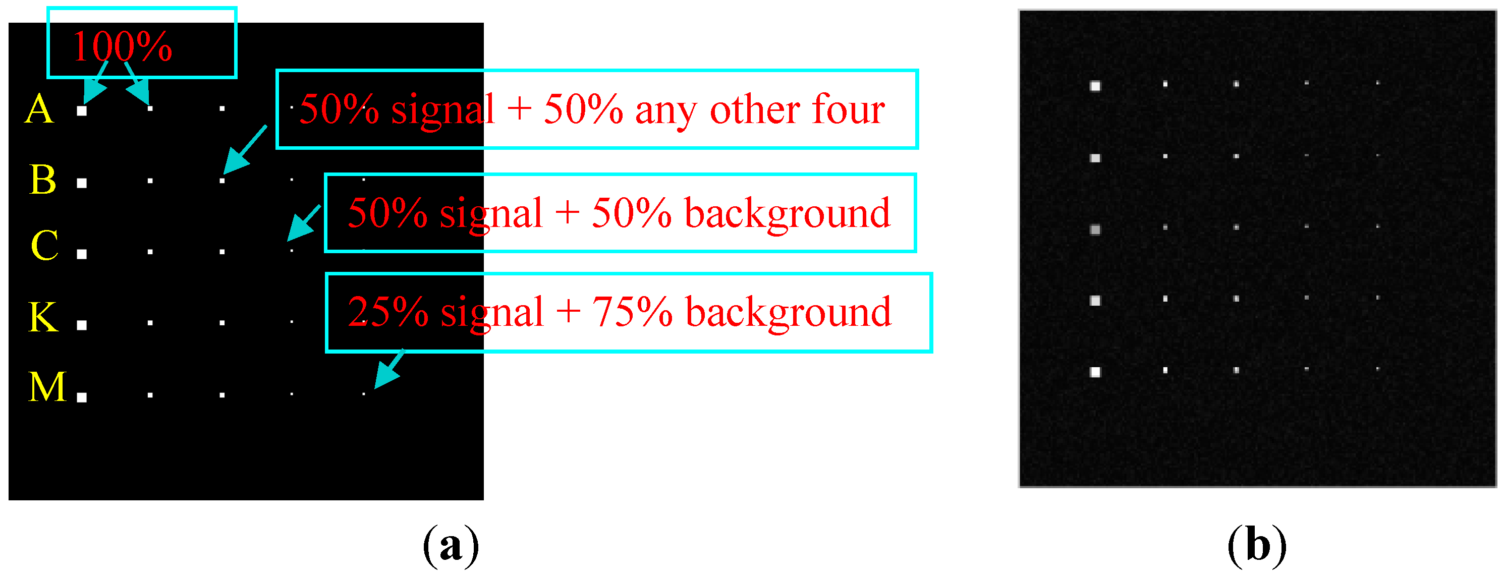
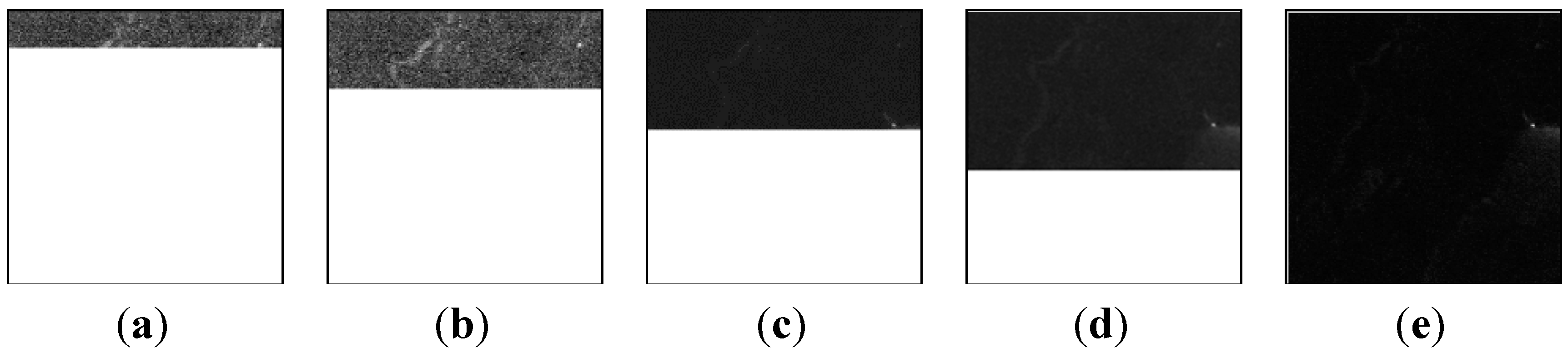
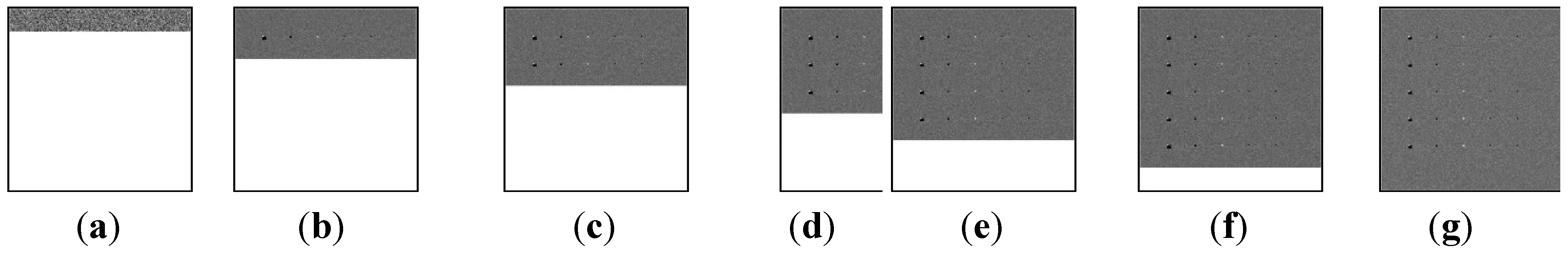
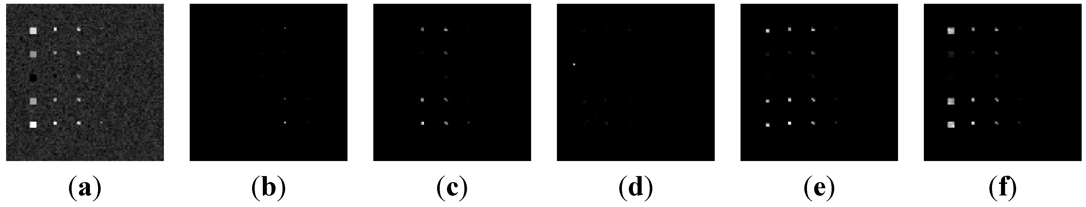
4.3. Local Real-Time Processing Experiments

Another question of interest derives from local anomaly detection: “what is the performance impact of the local window size on anomaly detection?” As in the previous section, before conducting the local real-time processing experiments, several experiments using TI images were conducted to explore this question. Figure 14 shows the LRXD results using different local window size with image size. When the inner window size equals 1, only the pixels in the 4th column could be detected, as shown in Figure 14a. When the inner window size increases to 3, the targets in the 2nd and 3rd columns could also be detected, as shown in Figure 14b. However, when the window size equals 5 or 7, the 1st column targets appeared on the grayscale results, as shown in Figure 14c–e. Comparing Figure 14a–e, it is clearly proved that the inner window size depends on the size of anomaly targets and the outer window size is much larger than the inner window size. The detection results get better from Figure 14a through Figure 14e. Figure 15 repeats the same experiments with image size. Comparing the corresponding sub-figures of Figure 14 and Figure 15, we could know that the image size will also affect the detection results.
Figure 14. LRXD results using different local window size with image size 200 × 200:(a) window size 1/15 (inner window size 1 and outer window size 15); (b) window size 3/15; (c) window size 5/15; (d) window size 5/17; (e) window size 7/17.
Remotesensing 07 03966 g014
Figure 15. LRXD results using different local window size with image size 100 × 100:(a) window size 1/15 (inner/outer window); (b) size 3/15; (c) size 5/15; (d) size 5/17;(e) size 7/17.
Remotesensing 07 03966 g015
The following experiments are conducted to verify the effectiveness of the local real-time detector using synthetic HSI data. Local AD concept is very important, as we said at the beginning, especially when global AD algorithms fail to detect targets that are extremely small or only abnormal in a local background but buried in the global background. Figure 16 is a very good explanation for this pattern. Figure 16a is generated using the same way Figure 5a does, but changes the order of A, B, C, K, M to K, A, M, B, C. Since material C is the nearest matching with the background signature (shown in Table 2), running with global real-time processing in Figure 16b, anomalies with C signature in the 5th row is hardly seen in the scene. However, when local real-time procedure is conducted to the same image (with causal array window size 15 × 15), all the anomalies could be well defined except for the 2 × 2-mixed pixel panels in the third column, much better than the global real-time detector. Figure 16d is the same detector with causal array window size 21 × 21, in which the 2 × 2-mixed pixel panels in the third column could be detected. Figure 17(a–g) are steps of local real-time causal array RXD detection results.
Figure 16. Local real-time anomaly detection experiments: (a) synthetic data scene; (b) global real-time causal RXD anomaly detection results; (c) local real-time causal array RXD anomaly detection results with array window width 15 × 15, (d) local real-time causal array RXD anomaly detection results with array window width 21 × 21.
Remotesensing 07 03966 g016
Table 2. Comparative analysis of spectral similarity between background and fivetarget signatures.
MeasuresAlunite (A)Buddingtonite (B)Calcite (C)Kaolinite (K)Muscovite (M)
SAM0.18210.06560.04410.19230.0924
SID0.04050.00460.00250.05220.0103
Figure 17. Gray scale detection results of local real-time causal array RXD: (a) no panels detected; (b) row 1 panels detected; (c) row 2 panels detected; (d) row 3 panels detected; (e) row 4 panels detected; (f) row 5 panels detected; (g) final detection result.
Remotesensing 07 03966 g017

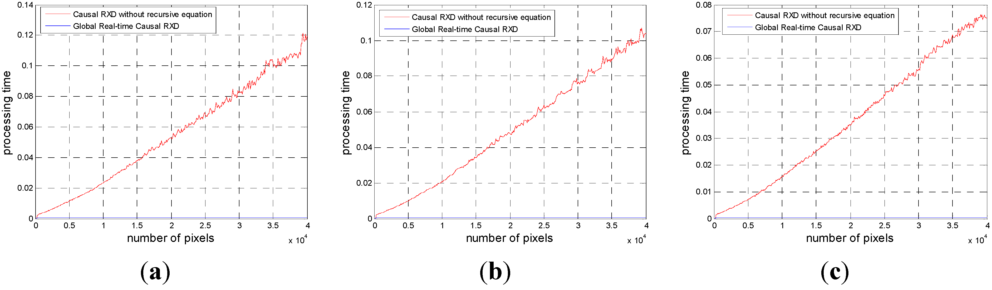
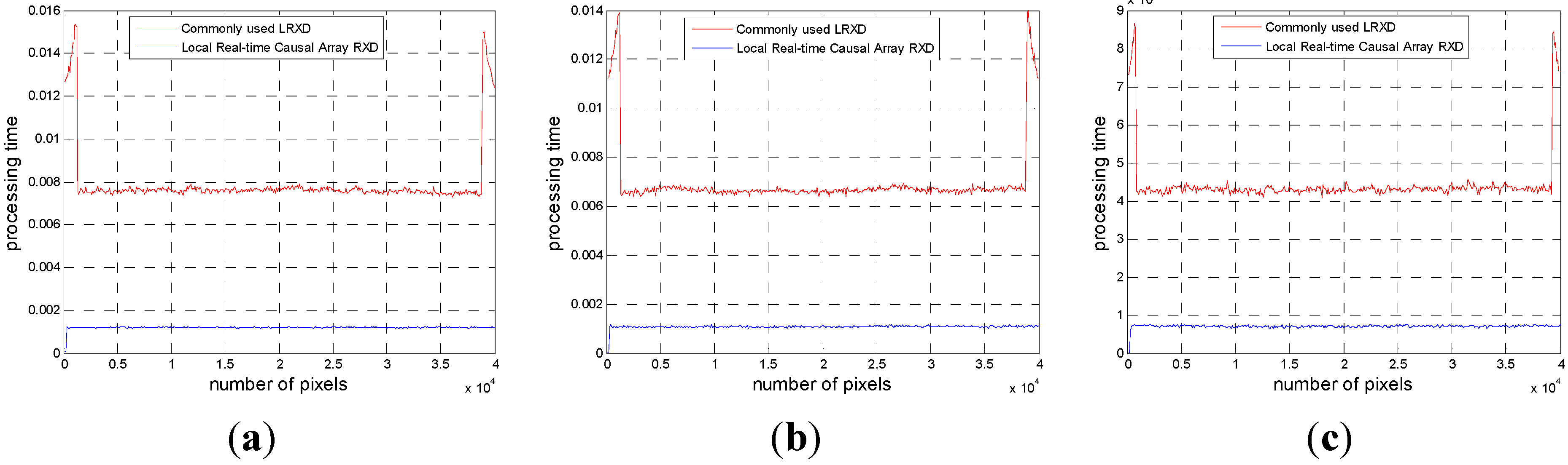
4.4. Computational Analysis

Computational complexity is also an important topic for HSI anomaly detection algorithms. The computational complexity of RX-based algorithms stems from the inversion of the covariance matrix that is required for the background estimation, which in general is of order O(L3), where L is the number of bands according to Table 2. For global anomaly detection algorithms, due to the requirement ofreal-time processing, the global background information (covariance/correlation matrix and its inversion) is re-calculated for each pixel. For local anomaly detection algorithms, on the other hand, this inversion is also required at every pixel due to the local nature of background estimation in a sliding local window at each spatial location in the hypercube. In this case, without using our new methodology, the total processing is of order O(NL3), where N is the total number of spatial pixels in the HSI scene. This results in a high computational cost, which could be reduced by using the Woodbury matrix identity in our real-time detectors.
The computer environments used for experiments are 64- bit operating systems with Intel(R) Core (TM) i7-4770K, 3.5 GHz CPU, and 16 GB memory (RAM). All the experiments were conducted five times and averaged to remove computer error. The average computing times (CPT) for both synthetic and real hyperspectral images are given in Table 3 using all detectors including global detectors (K-RXD, R-RXD, CRXD, GRTCRXD) and local detectors (LRXD, LRTCARXD). From Table 3 we could see that, using our new recursive equations, both global and local processing times were much reduced, especially the GRTCRXD, which was reduced by 100-fold compared with CRXD without recursive equation.
Table 3. Total processing time for TI, TE, and LCVF.
K-RXD
(seconds)
R-RXD
(seconds)
CRXD
(seconds)
GRTCRXD
(seconds)
LRXD
(seconds)
LRTCARXD (seconds)
Scenario TI1.70671.18252178.9724.1223332.839947.8953
ScenarioTE1.47891.10451984.9222.4953294.229443.1142
AVIRIS LCVF1.22930.79251471.5114.9151183.247628.1530
In order to further evaluate computational complexity, Figure 18 and Figure 19 give the averaged CPT for each pixel using both global and local detectors, where the x-axis and y-axis represent the order of pixels being processed and the CPT required for the current pixel, respectively.
Figure 18. CPT (Computing time) for global detectors. (a) TI image; (b) TE image; (c) LCVF image.
Remotesensing 07 03966 g018
Figure 19. CPT (Computing time) for local detectors. (a) TI image; (b) TE image; (c) LCVF image.
Remotesensing 07 03966 g019
For the global detectors in Figure 18, the data clearly show that the CPT that results from using the recursive updating equations specified by Equation (9) is much reduced, while the CPT from the CRXD algorithm linearly increased with the number of data sample vectors processed. Similar to Figure 19 for the local detectors, they also clearly show that the real-time version local detector has much reduced CPT compared with the commonly-used LRXD provided in Figure 1. It should be noted that the commonly-used LRXD CPT of the first and last few pixels plotted in Figure 19 is a little high, resulting from the boundary extension by local window principle in Figure 1.

5. Conclusions

This paper presents both global and local real-time algorithms for anomaly detection in hyperspectral imagery. RX detector is selected as the benchmark theory in this paper. Taking advantage of the Woodbury matrix identity, the proposed global and local detectors can be implemented and processed pixel-by-pixel in a real-time manner. The contributions of this work are summarized as follows:
  • The proposed real-time algorithm has two main features: (1) it is a causal procedure, in the sense that the data samples used for data processing should be only those up to the data sample vector currently being processed; (2) the processing time of the algorithm is negligible, and the proposed method could meet the efficiency requirement by updating the inverse of the correlation matrix without repeated recalculation. Taking advantage of these two features, we gain the benefit of saving data storage since it only needs to store two types of information, about the previous moment and pixel the currently being processed; this is also much easier in terms of hardware implementation because it uses an update equation instead of matrix inversion calculation.
  • As demonstrated in anomaly detection results for both synthetic and real hyperspectral images, real-time processing offers the significant advantage of seeing time-varying changes in background information. As time moves along, various levels of background suppression produce false alarms, thus producing a tremendous effect on visual assessment. This issue is worth pursuing and beyond the scope of this paper. It would be interesting to investigate this issue since background suppression provides users with a better understanding of what the detected anomalies really are. Specifically, some weak anomalies detected earlier may be overwhelmed by strong anomalies detected later, as the experimental results show. However, this phenomenon is very important in anomaly detection but cannot be observed using commonly used anomaly detectors, which perform one-shot operation to show the final detected anomalies.
  • Despite the fact that local anomaly detection for hyperspectral imagery is not new and has been widely discussed in the literature, the concept of a causal matrix local window (CMLW) and a causal array local window (CALW) for real-time implementation is new.
  • The Woodbury matrix identity has been known for a long time but is newly used to derive a recursive equation in this paper, avoiding computing reversion of covariance/correlation matrix. This will greatly shorten the processing time. Computational complexity analysis is very important for anomaly detection because some targets, especially moving targets, provoke immediate decision-making because they may show up suddenly and then disappear quickly afterwards. As a result, for this kind of detection, the processing time must be very short. This paper gives a comparative discussion of the computing time of different algorithms, showing the advantages of time-saving through the Woodbury matrix identity theory.
  • The proposed real-time detection methods have the additional benefit of being portable. Other detection algorithms, such as CEM, TCIMF, etc., could also be conducted as real-time detectors using the same methodology.

Acknowledgments

The authors would like to thank Professor Chein-I Chang for his help and guidance, and also for the study within his lab. This study was partially supported by the National Natural Science Foundation of China (No. 61405041, No. 61275010), the China Postdoctoral Science Foundation (Grant No. 2014M551221), the Heilongjiang Postdoctoral Science Found (Grant No. LBH-Z13057), the Key Program of Heilongjiang Natural Science Foundation (No. ZD201216), Program Excellent Academic Leaders of Harbin (No. RC2013XK009003), and the Fundamental Research Funds for the Central Universities (No. HEUCF1408).

Author Contributions

All authors assisted in the analyzing and editing of the paper. Yulei Wang is the main author who processed the data, developed the methodology, analyzed the results and wrote the manuscript. All authors reviewed and approved the final manuscript.

Conflicts of Interest

The authors declare no conflict of interest.

References

  1. Chang, C.-I. Hyperspectral Imaging: Techniques for Spectral Detection and Classification; Kluwer Academic/Plenum Publishers: New York, NY, USA, 2003. [Google Scholar]
  2. Chang, C.-I. Hyperspectral Data Processing: Algorithm Design and Analysis; Wiley: Hoboken, NJ, USA, 2013. [Google Scholar]
  3. Rosario, D.S. Algorithm Development for Hyperspectral Anomaly Detection. PhD Thesis, University of Maryland, College Park, MD, USA, 2008. [Google Scholar]
  4. Reed, I.S.; Yu, X. Adaptive multiple-band CFAR detection of an optical pattern with unknown spectral distribution. IEEE Trans. Signal. Process. 1990, 38, 1760–1770. [Google Scholar] [CrossRef]
  5. Plaza, A.; Martinez, P.; Plaza, J. A new method for target detection in hyperspectral imagery based on extended morphological profiles. In Proceedings of the 2003 IEEE International Conference on Geoscience and Remote Sensing Symposium, Toulouse, France, 21–25 July, 2003; pp. 3772–3774.
  6. Kwon, H.; Nasrabadi, N.M. Kernel RX-algorithm: A nonlinear anomaly detector for hyperspectral imagery. IEEE Trans. Geosci. Remote Sens. 2005, 43, 388–397. [Google Scholar] [CrossRef]
  7. Foy, B.R.; Theiler, J.; Fraser, A. M. Decision boundaries in two dimensions for target detection in hyperspectral imagery. Opt. Express. 2014, 22, 608–617. [Google Scholar] [CrossRef] [PubMed]
  8. Guo, Q.; Zhang, B.; Ran, Q.; Gao, L.; Li, J.; Plaza, A. Weighted-RXD and linear filter-based RXD: Improving background statistics estimation for anomaly detection in hyperspectral imagery. IEEE J. Sel. Top. Appl. Earth Obs. Remote Sens. 2014, 7, 2351–2366. [Google Scholar] [CrossRef]
  9. Kwon, H.; Der, S.Z.; Nasrabadi, N.M. Projection-based adaptive anomaly detection for hyperspectral imagery. In Proceedings of the 2003 IEEE International Conference on Image Processing, Barcelona, Spain, 14–17 September, 2003; pp. 1001–1004.
  10. Ranney, K.I.; Soumekh, M. Hyperspectral anomaly detection within the signal subspace. IEEE Geosci. Remote Sens. Lett. 2006, 3, 312–316. [Google Scholar] [CrossRef]
  11. Ma, L.; Crawford, M.M.; Tian, J. Anomaly detection for hyperspectral images using local tangent space alignment. In Proceedings of the 2010 IEEE International Conference on Geoscience and Remote Sensing Symposium, Honolulu, HI, USA, 25–30 July, 2010; pp. 824–827.
  12. Taitano, Y.P.; Geier, B.A.; Bauer, K.W., Jr. A locally adaptable iterative RX detector. Eurasip. J. Adv. Sign. Process. 2010. [Google Scholar] [CrossRef]
  13. Matteoli, S.; Diani, M.; Corsini, G. A kurtosis-based test to efficiently detect targets placed in close proximity by means of local covariance-based hyperspectral anomaly detectors. In Proceedings of the 3rd Workshop on Hyperspectral Image and Signal Processing: Evolution in Remote Sensing, Lisbon, Portugal, 6–9 June, 2011.
  14. Molero, J.M.; Garzon, E.M.; Garcia, I.; Plaza, A. Analysis and optimizations of global and local versions of the RX algorithm for anomaly detection in hyperspectral data. IEEE J. Sel. Top. Appl. Earth Obs. Remote Sens. 2013, 6, 801–814. [Google Scholar] [CrossRef]
  15. Kwon, H.; Der, S.Z.; Nasrabadi, N.M. Adaptive anomaly detection using subspace separation for hyperspectral imagery. Opt. Eng. 2003, 42, 3342–3351. [Google Scholar] [CrossRef]
  16. Matteoli, S.; Veracini, T.; Diani, M.; Corsini, G. A locally adaptive background density estimator: An evolution for RX-based anomaly detectors. IEEE Geosci. Remote Sens. Lett. 2014, 11, 323–327. [Google Scholar] [CrossRef]
  17. Scholkopf; Smola, A.J. Learning with Kernels; MIT Press: Cambridge, MA, USA, 2002. [Google Scholar]
  18. Chang, C.-I.; Chiang, S.-S. Anomaly detection and classification for hyperspectral imagery. IEEE Trans. Geosci. Remote Sens. 2002, 40, 1314–1325. [Google Scholar] [CrossRef]
  19. Ren, H.; Chang, C.-I. Target-constrained interference-minimized approach to subpixel target detection for hyperspectral images. Opt. Eng. 2000, 39, 3138–3145. [Google Scholar] [CrossRef]
  20. Wang, Y.; Schultz, R.; Chen, S.; Liu, C.; Chang, C.-I. Progressive constrained energy minimization for subpixel detection. Proc. SPIE 2013, 8743, 874321. [Google Scholar]
  21. Liu, W.; Chang, C.-I. A nested Spatial window-based approach to target detection for hyperspectral imagery. In Proceedings of 2004 IEEE International Conference on Geoscience and Remote Sensing Symposium, Anchorage, AK, USA, 20–24 September, 2004; pp. 266–268.
  22. Liu, W.; Chang, C.-I. Multiple-window anomaly detection for hyperspectral imagery. IEEE J. Sel. Top. Appl. Earth Obs. Remote Sens. 2013, 6, 644–658. [Google Scholar] [CrossRef]
  23. Stellman, C.M.; Hazel, G.G.; Bucholtz, F.; Michalowicz, J.V.; Stocker, A.; Scaaf, W. Real-time hyperspectral detection and cuing. Opt. Eng. 2009, 17, 17391–17411. [Google Scholar]
  24. Zhao, C.; Wang, Y. Design and analysis of hyperspectral anomaly detection based on Kalman filter theory. Chin. J. Electron. 2013, 22, 849–854. [Google Scholar]
  25. Molero, J.M.; Garzon, E.M.; Garcia, I.; Quintana-Orti, E.S.; Plaza, A. Efficient implementation of hyperspectral anomaly detection techniques on GPUs and multicore processors. IEEE J. Sel. Top. Appl. Earth Obs. Remote Sens. 2014, 7, 2256–2266. [Google Scholar] [CrossRef]
  26. Rossi, A.; Acito, N.; Diani, M.; Corsini, G. RX architectures for real-time anomaly detection in hyperspectral images. J. Real-Time Image Process. 2012. [Google Scholar] [CrossRef]
  27. Ensafi, E.; Stocker, A. D. An adaptive CFAR algorithm for real-time hyperspectral target detection. Proc. SPIE 2008. [Google Scholar] [CrossRef]
  28. Hager, W.W. Updating the inverse of a matrix. SIAM Rev. 1989, 31, 221–239. [Google Scholar] [CrossRef]
  29. Press, W.H.; Teukolsky, S.A.; Vetterling, W.T.; Flannery, B.P. Numerical Recipes: The Art of Scientific Computing, 3rd revised ed.; Cambridge University Press: Cambridge, UK, 2007. [Google Scholar]
  30. Chen, S.; Wang, Y.; Wu, C.; Liu, C.; Chang, C.-I. “Real-time causal processing of anomaly detection for hyperspectral imagery. IEEE Trans. Aerosp. Electron. Syst. 2014, 50, 1511–1534. [Google Scholar] [CrossRef]
  31. USGS Website. Available online: http://speclab.cr.usgs.gov/cuprite.html (accessed on 27 July 2014).
  32. Chang, C.-I.; Hsueh, M. Characterization of anomaly detection for hyperspectral imagery. Sens. Rev. 2006, 26, 137–146. [Google Scholar] [CrossRef]

