Article

Using a Remote Sensing-Supported Hydro-Agroecological Model for Field-Scale Simulation of Heterogeneous Crop Growth and Yield: Application for Wheat in Central Europe

1
Department of Geography, Ludwig-Maximilians-Universität Munich, Luisenstraße 37, 80333 Munich, Germany
2
VISTA Remote Sensing in Geosciences, Gabelsbergerstraße 51, 80333 Munich, Germany
*
Author to whom correspondence should be addressed.
Remote Sens. 2015, 7(4), 3934-3965; https://doi.org/10.3390/rs70403934
Submission received: 30 September 2014 / Revised: 17 March 2015 / Accepted: 26 March 2015 / Published: 1 April 2015

Abstract

:
The challenge of converting global agricultural food, fiber and energy crop cultivation into an ecologically and economically sustainable production process requires the most efficient agricultural management strategies. Development, control and maintenance of these strategies are highly dependent on temporally and spatially continuous information on crop status at the field scale. This paper introduces the application of a process-based, coupled hydro-agroecological model (PROMET) for the simulation of temporally and spatially dynamic crop growth on agriculturally managed fields. By assimilating optical remote sensing data into the model, the simulation of spatial crop dynamics is improved to a point where site-specific farming measures can be supported. Radiative transfer modeling (SLC) is used to provide maps of leaf area index from Earth Observation (EO). These maps are used in an assimilation scheme that selects closest matches between EO and PROMET ensemble runs. Validation is provided for winter wheat (years 2004, 2010 and 2011). Field samples validate the temporal dynamics of the simulations (avg. R² = 0.93) and > 700 ha of calibrated combine harvester data are used for accuracy assessment of the spatial yield simulations (avg. RMSE = 1.15 t∙ha−1). The study shows that precise simulation of field-scale crop growth and yield is possible, if spatial remotely sensed information is combined with temporal dynamics provided by land surface process models. The presented methodology represents a technical solution to make the best possible use of the growing stream of EO data in the context of sustainable land surface management.

Graphical Abstract

1. Introduction

The challenge of sustainably providing food, fiber and energy from limited resources for an increasing world population requires a most efficient use of the biologically productive land surface. Ecologically and economically efficient agricultural management thereby is highly dependent on detailed temporal and spatial knowledge of the processes affecting physiological crop development. Management techniques that make use of this detailed knowledge are summarized under the term “Precision Agriculture”, which is becoming an increasingly important part of smart farming practices [1,2,3]. Understanding natural heterogeneity patterns is the basis of all site-specific management decisions in the context of precision agriculture. Data on spatial heterogeneity of fields, though essential, can hardly be acquired with conventional in situ methods due to restrictions such as labor intensity, limited accessibility of large continuous acreages, crop damage through destructive sampling etc. In situ measurements, although essential for process understanding, can only be provided for selected sampling points and thus largely fail to represent the natural heterogeneity of growth conditions that can be found within the boundaries of agricultural fields.
When it comes to observing spatial heterogeneities in plant development, biomass accumulation and yield, very few tools are available. GPS-equipped harvesters give detailed information on the heterogeneity of the harvest through more or less direct measurements at the end of the growing season [1]. However, they are not available to the majority of farmers, they are very sensitive to calibration and inter-calibration, they are not capable of measuring more than one field at a time and, most significantly, cannot be applied during the growing season to determine plant development and yield formation. Their relevance for decision support therefore is limited. Remote sensing, as the tool for spatially continuous measurements [4], allows for an indirect observation of spatial growth patterns through their effect on canopy reflectance. The reflectance behavior of agricultural canopies is mainly determined by the biochemical and structural state of the crop, which is a result of, for instance, the development of leaves, accumulation of pigments such as chlorophyll, and progressing phenological development with impact on leaf angle distribution [5]. However, for agricultural management, remote sensing comes at the expense of an indirect determination of the parameters of interest. Optical earth observation (EO) data are mostly used for agricultural applications despite their weather dependency (clouds, haze), since sub-field applications of SAR data for in-field heterogeneity are only about to be explored [6]. In the optical domain, simple spectral indices are commonly used. These indices require correlations with in situ measurements in order to retrieve quantitative information from these relative estimators of crop status. Measuring absolute biomass for specific dates solely based on satellite observations remains difficult [7].
Spatially explicit process models enable numerical simulations of the mass and energy balance at the land surface. While some simplified models exist that are designed for simulation of vegetation growth at the global scale [8,9,10] and detailed models of plant growth have been developed for the point scale [11,12,13], field scale simulation studies on heterogeneous vegetation growth are seldom found. At the same time, numerous spatially distributed hydrological models [14,15,16,17] are applied in regional scale studies. Their performance is usually validated against measured runoff data [18,19,20]. However, spatially distributed hydrological models mostly rely on a rather coarse and parameterized representation of land surface processes and specifically of vegetation. This paper aims at bridging this gap by extending an existing spatially explicit hydrological model (PROMET) [20] with a highly sophisticated representation of dynamic vegetation processes at the land surface and by using the coupled model for the assimilation of remote sensing observations. The advantage of using PROMET thereby lies in the generic spatial focus of the model, evolving from the hydrological background, as well as in its capability of describing diurnal dynamics by calculating hourly time-steps.
Crop growth models alone cannot produce yield maps with adequate accuracy for practical applications since the spatial detail of input data is hardly sufficient [21]. Accordingly the integrated use of remote sensing in crop modeling for yield prediction started already in the 90ies of the previous century [22,23]. Since then, the methods to derive biophysical canopy state variables from optical remote sensing data have developed from statistical-empirical to physical-based methods [24]. Various applications can be found in literature for different crop types and regions using various data assimilation schemes like the Kalman filter [25], ensemble techniques [26] or model re-initialization [27]. However, these examples are based on medium resolution satellite data (MODIS, MERIS) and valid only for regional assessments. At the field scale, calibrated crop growth models are often applied together with empirical relations [28] or Neural Networks [29] for Leaf Area Index (LAI) retrieval. This limits the transferability of these approaches. Accordingly, our paper aims at presenting a methodology based on high resolution data and simulation that is relevant to precision farming (i.e., 20 m resolution). A model environment is applied that uses physically based approaches and a fixed set of internal model parameters that are not calibrated for the specific case. Multiyear spatial validation was performed using detailed yield maps of two farms in central Europe. Wheat was selected for demonstration as one of the major crops relevant for food security. The generic approach is, however, transferable to all major crop types.

2. Materials and Methods

2.1. Study Area

The results shown in this study were achieved in two different test regions in Germany, which show differences with respect to climate, soils and management. Due to the proximity of the climatic barrier of the Alps, humid conditions prevail in the southern test area near the city of Munich (48.09° N, 11.32° E), long-term annual rainfall accumulating to approximately 900 mm per year. The northern test area (51.86° N, 10.95° E) is positioned leeward of the Harz Midrange Mountains and therefore receives significantly less precipitation with annual sums of rainfall regularly not exceeding 450 mm. From an agricultural perspective, this locational disadvantage is neutralized to some extent by the existence of rich and fertile soils, mostly Chernozems (according to the World Reference Base for Soil Resources [30]), providing favorable conditions for crop cultivation. The land management strategies applied in northeastern Germany during the existence of the former German Democratic Republic led to the establishment of large continuous acreages that currently allow for a highly mechanized crop production in the region. Quite in contrast, the agricultural landscape of southern Germany is rather small-parcelled and thus does not allow for a highly optimized large scale crop production, although productive soils prevail, consisting predominantly of Luvisols developed from Loess sediments. Main crops in both test areas are winter wheat followed by rapeseed and maize.

2.2. The Hydro-Agroecological Land Surface Model PROMET

The goals of the study require a coupled hydro-agroecological model, which is capable of tracing the temporal dynamics and spatial heterogeneities of coupled water and carbon fluxes at the scale of agricultural fields. In order to enable the model’s application as decision-support tool for farming, field-wise calibration must be avoided and predictive abilities should be strengthened. This can be achieved by using physical, biochemical and plant physiological principles for crop growth modeling, governed by fixed crop-specific parameters. High-resolution local information is integrated by remote sensing observations that mirror the true natural variability. This eliminates the need for site-specific or variety-specific calibration.

2.2.1. Model Parameterization

The coupled model allows for the simulation of heterogeneous crops as well as natural vegetation in a generic way by using detailed crop-specific parameterizations. A total of 18 agricultural crop types are supported at present (winter wheat, summer wheat, winter barley, summer barley, millet, rye, maize, maize silage, paddy rice, soybeans, sorghum, sunflower, sugar beet, sugar cane, potatoes, rapeseed, cassava, ground nut). The required parameters were derived from literature where available and complemented from own measurements and observations. The parameterization of the photosynthesis model was taken from [31] for C3 grasses and connatural cereals, while the carboxylation of C4 plants is parameterized according to [32]. The growth stage-dependent distribution of biomass to the different plant fractions mostly follows the allocation percentages applied in the CERES crop growth models [33,34] for the agricultural land use categories. For this study, we concentrate on winter wheat. Parameters applied for the calculations of winter wheat growth in this study are listed in Table 1 and Table 2.
A comprehensive description of the algorithms used in the coupled model can be found in [35]. The degree of detail would even allow for a variety-specific parameterization of the wheat crops. However, this option was not used in his study, since information on varieties is hardly available and variations of crop development caused by differences in the variety will be considered through the assimilation of Earth Observation data.

2.2.2. Hydrological Core Model

For the hydrological part of the coupled model, the Process of RadiatiOn Mass and Energy Transfer model (PROMET) [20] was chosen. It is a raster-based model system that has been designed by the authors to spatially simulate the elements of the land surface water balance including soil moisture and river discharge. PROMET incorporates a four-layer soil model, which is based on the explicit solution of the Richards equation [36] and considers lateral flows along hill slopes. Due to its raster-based architecture, the model allows for the assimilation of remote sensing data for distributed hydrological applications [37]. PROMET solves the water and energy balance for hourly time steps and calculates the runoff of river basins, while it strictly conserves mass and energy. It thus allows for the validation of the complete process chain, from rainfall over soil-moisture dynamics to vegetation controlled evapotranspiration and finally routed runoff, against measured discharges on the basin and sub-basin scale. PROMET has successfully been applied for a variety of hydrological studies in medium- to large-sized watersheds [20,37,38,39,40]. Required input data consists of raster-based GIS information, characterizing the spatial distribution of land use patterns, soil types and topographic features. In addition, parameters describing the characteristics of the discerned soil and land use/crop categories are supplied through tabular input. In this study, spatially interpolated time series of meteorological station network records are used as driving meteorological parameters. However, the model is also equipped with interfaces that allow for a coupling with global and regional climate models [41,42]. To enable the use of PROMET for agroecological studies at the field scale, PROMET has been extended by a detailed model of plant physiological processes, canopy development and agricultural management [35]. The enhanced parts of the PROMET model are highlighted in Figure 1.
Figure 1. Internal design of the enhanced PROMET agroecological land surface model. The extended model components relevant for this study are highlighted in green.
Remotesensing 07 03934 g001

2.2.3. Leaf Photosynthesis

Comparable to some of the globally applied dynamic vegetation models (e.g., HYBRID [43], IBIS [8], LPJ [9]), we base the description of the photosynthetic processes on the Farquhar et al. approach [31]. The Farquhar et al. model of photosynthesis can be considered to be the most widely known and most successfully applied model to describe the processes related to photosynthesis at the chloroplast scale [44]. Although the model initially was developed in the laboratory as a not strictly mechanistic tool and therefore rather represents a semi-empirical rather than a physically based hypothesis [45], it has recently developed into a well-accepted mechanism-oriented photosynthesis model. PROMET describes net photosynthesis (np) according to [31] as shown in Equation (1),
n p = ( 1 Γ * C i ) M I N { w c ; w j } 0.5 × r d
where the term 0.5 × rd represents the fraction of the dark respiration (rd) during daytime, which can best be described as the mitochondrial respiration, the symbol Γ* stands for the CO2 compensation point, i.e. the assimilation rate where the oxygen production of the photosynthesis process exceeds the oxygen demand of the mitochondrial respiration, and Ci is the CO2 concentration within the leaf. The net photosynthesis rate is assumed to be limited by two determinant situations wc and wj.
For low CO2 concentrations within the leaf, the fixation rate of RuBisCO and the competition of CO2 and O2 determine the assimilation rate, as shown in Equation (2),
w c = V c max c i c i + K c ( 1 + O 2 K o )
where Vcmax is the maximum carboxylation velocity, Kc and Ko are the Michaelis-Menten constants for CO2 and O2 respectively and O2 is the leaf internal concentration of oxygen given in Table 1.
For high CO2 concentrations, the photosynthesis rate is only limited by the rate of the electron transport or the rate of RuBP regeneration respectively as described in Equation (3), where Pm is the light-dependent rate of photosynthesis at saturated CO2:
w j = p m 1 + 2 Γ * C i
The CO2 compensation point Γ*, as well as wc and Pm (with effect on wj) are dependent on the maximum carboxylation velocity Vcmax, which is calculated though an Arrhenius function (Equation (4)) in dependence of the leaf temperature Tl:
V c max ( T l ) = [ V c max 25 e E a V c max ( T l 298.16 ) 298.16 R T l ( 1 + e 298.16 Δ s E a V c max 298.16 R 1 + e T l Δ s E d V c max T l R ) ] × N s t a t u s
Table 1. PROMET Model parameters and variables applied for the simulation of winter wheat growth.
ParameterSymbolWinter Wheat (C3)Physical Unit
Light Use Efficiencyα0.045[mol CO2 mol photons−1]
CO2 Compensation PointΓ*variable[μl∙l−1]
CO2 Concentration in the LeafCivariable[ppm]
Harvest DateDhar206−237[DOY]
Day Light Effect (Photoperiodism)DLElong-day[–]
Entropy FactorΔs660.0[–]
Sowing DateDsow278–304[DOY]
Activation Energy for C KineticsEaVcmax79430.0[J∙mol−1]
Deactivation Energy for C KineticsEdVcmax198,000.0[J∙mol−1]
Stomatal Sensitivity Parametergfac10.6[–]
Max. Rate of Electron Transport at 25 °CJmax2532.3[µmol∙e−1∙m−2 leaf area∙s−1]
Michaelis-Menten-Constant for C at 25 °CKc25404.9[ml∙l−1]
Michaelis-Menten-Constant for O at 25 °CKo25278.4[ml∙l−1]
Relation LAI to Canopy HeightLHrel0.178[m∙m−2 leaf area]
Leaf Mass AreaLMA0.0704[kg∙m−2 leaf area]
Leaf WidthLw0.015[m]
Minimum Light Period (Min. Day Length)MLP8.25[h]
Rate of Net Leaf Photosynthesisnpvariable[μmol∙m−2∙leaf area∙s−1]
Nitrogen StatusNstatus0.1–1.0[–]
Leaf Concentration of OxygenO2210[ml∙l−1]
Light-Dependent Rate of PhotosynthesisPmvariable[μmol∙m−2 leaf area∙s−1]
Photoperiod Sensitivitypsen0.3[1/h]
BBCH-Threshold 00–50PTthres 00–500.01/0.20/0.30/0.60/0.67[–]
BBCH-Threshold 60–90PTthres 60–900.80 / 1.00 / 1.60 / 1.90[–]
Gas ConstantR8.31 [J K1 mol1]
Rate of Dark Respirationrdvariable[μmol∙m−2 leaf area∙s−1]
Respiration Capacity at 25 °Crd250.93[µmol∙m−2 leaf area∙s−1]
Maximum Root DepthRmax150[cm]
Cardinal Temp. (vegetative)Tb / To / Tc 10 / 19 / 30[°C]
Cardinal Temp. (generative)Tb / To / Tc 24 / 24 / 35[°C]
Cardinal Temp. (maturity)Tb / To / Tc 38 / 24 / 35[°C]
Leaf TemperatureTlvariable[K]
Maximum Carboxylation CapacityVcmaxvariable[µmol∙m−2 leaf area∙s−1]
Carboxylation Capacity at 25 °CVcmax2568.1[µmol∙m−2 leaf area∙s−1]
Vernalisation TemperaturesVnTb / VnTo / VnTc−1.3 / 4.9 / 15.7[°C]
Assimilation Rate at Low CO2wcvariable[μmol∙m−2 leaf area∙s−1]
Assimilation Rate at Saturated CO2wjvariable[μmol∙m−2 leaf area∙s−1]
Yield FactorYF0.73[fraction]
Max. Dev. Rate (veg., gen., mat.)ωmax0.06 / 0.0285 / 0.03[–]
Here, Vcmax25 is the carboxylation capacity at 25 °C and EaVcmax and EdVcmax are the activation and deactivation energies of the process, Δs is an entropy factor according to [46] and R stands for the gas constant as given in Table 1. We further assume that the maximum carboxylation capacity is limited by the status of nitrogen supply Nstatus. Five environmental variables govern photosynthesis in the model: (1) availability of photosynthetically active radiative energy, (2) leaf temperature, (3) concentration of CO2 within the leaf, (4) provision of soil water, and (5) nitrogen status. While the leaf temperature is a result of the leaf energy balance, the concentration of CO2 in the leaf mesophyll is the result of the concentration gradient between leaf and atmosphere as well as of the conductivity of the leaf surface. Both processes are variable in space and time, the spatial variability again being discerned into vertical and lateral variations. The rate of gas exchange on leaf level thereby strongly depends on the position of the leaf within the canopy. This has to be taken into account by implementing a dynamic canopy model, which describes canopy development in dependence of environmental variables.

2.2.4. Canopy Development

The canopy model first scales available energy, temperature and CO2 concentration from the atmosphere to the leaf level, thus creating a valid environment for the photosynthesis model. It then rescales the photosynthetic performance of the leaves back to the canopy level, thus enabling the simulation of canopy development.
It has been found by [47] that two-layer canopy models are superior to single layer models with respect to the modeling of sensible and latent heat flux above closed canopies. The canopy model of PROMET thereby is designed as a two-layer big-leaf model, where the energy-balances of the different layers are interdependently influencing each other. The energy balance at the leaf surface of each canopy layer is solved iteratively, based on the incoming (direct and diffuse shortwave and long wave radiation) and outgoing (reflectance, heat emission, conductive and latent heat) energy fluxes. The result of this iteration is an equilibrium leaf temperature, where the radiative energy gains equal the losses.
Depending on the canopy structure (canopy height, leaf area, leaf angle) and the solar input (aspect, zenith angle, cloud coverage), shaded and sunlit fractions are discerned for each canopy layer. For the incoming direct radiation, a random ellipsoidal distribution of the leaves is assumed and the interception of light is calculated according to [48]. Thermal emission of heat is calculated following the Stefan-Boltzmann-Law in dependence of the leaf temperature, taking into account that long-wave radiation is emitted on both sides of the leaf.
The sensible heat flux from the leaf then is calculated according to [49] in dependence of the width of the leaf and the wind velocity. Since all processes of heat transfer largely depend on the transport capacities of the surrounding air, the wind speed distribution in the canopy must be known. It is approximated assuming a logarithmic wind profile based on [50].
The third and most determinant loss of energy from the leaf is the amount of latent energy that is transported from the canopy via transpiration. It is calculated based on the actual transpiration rate assuming an approximation for the latent heat of vaporization after [49] for the respective leaf temperature. By balancing the radiative energy inputs (direct, diffuse, long wave) and the energy losses (emission, sensible heat, latent heat) at the leaf surface, the resulting leaf temperature is determined.
The primary driving force of transpiration is the vapor pressure gradient between the leaf and the surrounding air. Thereby, two barriers, the stomata-perforated cuticle and the boundary layer above the leaf surface, are inhibiting the flux of latent heat. The temperature-dependent conductance of the boundary layer for water vapor is described according to [49]. The conductance of the stomata is computed applying the Ball-Berry equation [51]. It empirically describes stomatal conductance as being influenced by the net photosynthesis rate, the relative humidity, the dark respiration, the minimum leaf conductance, the carbon dioxide concentration at the surface of the stomata and the factor gfac, which basically incorporates a linear response of stomatal conductance to net assimilation [52]. Since photosynthesis is strongly limited by the provision of carbon dioxide, the atmospheric carbon dioxide concentration within the leaf must be provided. Fick’s diffusion law is applied for the derivation of the CO2 concentration at the leaf surface, assuming a molecular diffusion between leaf surface and atmosphere within the boundary layer. Stomatal conductance is primarily regulated by the water supply, which is calculated in dependence of the provision of water from the soil water storage. PROMET simulates a four-layered soil column, where each layer may feature individual physical properties. This may lead to variable moisture conditions between the soil layers. Depending on the fraction of each soil layer that is accessed by the modelled root system, the inhibition due to the soil moisture status is calculated through a loading function following [53]. Apparently, the provision of water is determined by the root system. The growth rate of the roots therefore is modelled dynamically according to the amount of biomass that is distributed into the root fraction of the canopy. Dry conditions among the individual soil layers will inhibit root intrusion, so that layers of gravel, for instance, which, due to their limited storage capacities tend to be rather dry, may prevent the modelled canopy from accessing the moisture storage of deeper soil compartments. A weak nutrient concentration within the soil layers, i.e. an insufficient supply of nitrogen, will also inhibit root intrusion.

2.2.5. Crop Phenology and Biomass Allocation

The calculation of the latent heat flux not only requires the determination of the leaf temperature, but also the calculation of below ground biomass accumulation in order to provide a root system capable of accessing the soil water and nitrogen storage. The root mass develops in the model according to the amount of biomass that is distributed into the root fraction of the canopy. The same applies to the other parts of the canopy, such as the LAI, which develops in dependence of the leaf mass (LMA see Table 1 and Table 2). Since the leaf area represents the absolute interface surface between plant and atmosphere, the leaf area per ground unit is used for the scaling of the photosynthetic outputs first to the sunlit and shaded fractions of each canopy layer and finally up to the whole canopy. The distribution of biomass into the canopy fractions highly depends on the phenological stage of the crop.
The phenological progress of agricultural crops is modelled discerning consecutive growth stages corresponding to the BBCH phenological classification system [54]. A temperature and photoperiodic day-length-dependent approach is used. Following [12], the phenological progress is described as the crop-specific potential development rate (ωmax in Table 1). This rate is limited by crop-specific cardinal temperatures (Tb/o/c, b = base, o = optimum, c = ceiling), daylight requirements (DLE, MLP, psen) and, in the case of winter crops, vernalization phases (VnTb/o/c). Explicit phenological stages finally are discerned where crop-specific thresholds (PTthres) of accumulated development rates are exceeded. The model thus is capable of tracing inter-annual and topographic climate variations. Depending on the modelled growth stage, the total accumulated dry biomass is subdivided according to parameterized crop-specific percentages (Table 2) and is distributed into the canopy fractions leaf, stem, fruit, and root.
Table 2. Partitioning coefficients used for the allocation of assimilates into the winter wheat canopy fractions in dependence of the BBCH growth stage.
BBCH:00−0910−1920−2930−3941−4951−5961−6971−7783−8992−99
Fruit:0.0000.0000.0000.0000.0750.1000.5001.0001.0001.000
Leaf:0.0000.4250.4250.4000.1500.1000.0000.0000.0000.000
Stem:0.0000.0000.0000.2750.6750.7000.4000.0000.0000.000
Root:1.0000.5750.5750.3250.1000.1000.1000.0000.0000.000
By accumulating the generated and distributed biomass at each time step over the course of a growing season, a canopy may be modelled that is characterized by a certain growth stage, leaf area, canopy height, leaf mass, stem mass, fruit mass, root mass and root depth and root length density distribution.

2.2.6. Agricultural Management

A special challenge for the modeling of field-scale land surface processes is the integration of human activity that may be of hydrologic, climatic or agricultural consequence, such as sowing and harvesting. In PROMET, an agricultural management subroutine (Figure 1) initializes these major management actions. Perennial and non-perennial land cover types are thereby discerned, the non-perennial types again being classified into winter and spring crops. Sowing dates are mostly determined by long-term climate patterns, which lead to the development of regional traditions. The sowing date may be parameterized for individual crop types (e.g., Dsow in Table 1), while also spatial input of variable sowing dates is possible (e.g., field-wise). The same holds true for the harvest dates. Optionally, harvest dates can be modelled considering the simulated phenological stage of maturity and a drying period of two weeks. This dynamic harvesting process may lead to weather induced patterns of harvesting, even when uniform sowing dates were assumed. If the climatic conditions allow for the cultivation of multiple crops during one growing season, up to three repeated growth cycles per year can be modelled. Accounting for the management actions necessary for the replanting, such as ploughing, tilling, harrowing, seeding etc., gaps of at least two weeks are assumed between consecutive crop cycles.
By initializing the model through the crop-specific management actions and scaling the photosynthetic performance of the leaves to the canopy level, the biomass development is modelled for different crops. From an agricultural point of view, yield is of special interest. While for grassland and silage crops all of the accumulated aboveground biomass is harvested and therefore is considered as yield, only the belowground biomass is harvested from root crops, such as potato or sugar beet. For cereals and maize, all biomass that has been allocated to the fruit fraction of the canopy potentially contributes to the yield. Accounting for husks and dead material that is not directly considered as yield, a crop-specific yield factor (YF in Table 1) is used to reduce the biomass of the fruit compartment to the actual dry yield.

2.3. Assimilation of Earth Observation Data

The PROMET model requires four groups of model inputs that affect the spatial simulation of crop development at the field scale:
  • Agricultural management: farmers’ decisions on land use, sowing date, fertilization events, harvest date
  • Crop specifications: parameters that describe the crop and/or variety-specific physiological characteristics and the crops’ reactions to environmental variables (e.g., Table 1 and Table 2)
  • Dynamic environmental driver variables: temperature, precipitation, radiation, wind, atmospheric carbon dioxide concentration
  • Static environmental parameters: location, terrain, soil properties
Type 1 model parameters can be derived from Earth Observation [6,55] or are known from farm management documentations, statistics, or agronomical consultation systems. Type 2 parameters are largely described in the literature or may be generated from laboratory or plot experiments. Both parameter types 1 and 2 usually apply to the entire extent of a field, which is considered the basic agricultural management unit. Type 3 parameters may be measured at weather stations and can be provided spatially through interpolation, while type 4 parameters ordinarily are taken from available sources like soil- and terrain-maps, digital data sets generated from remote sensing or from field sampling data, respectively.
In order to link the spatio-temporal model with a high resolution remote sensing information stream, at least one spatial variable has to be identified, which can be determined through remote sensing and which can be spatially simulated by the model at the same time. We choose the photosynthetically active leaf area per ground unit (which we further denote by “greenLAI”) as this linking variable for two reasons: (1) A close relation between observed greenLAI variations and growth supporting locational advantages has been identified, e.g., by [56]. (2) PROMET spatially simulates greenLAI as a canopy variable in dependence of the leaf mass (see Section 2.2.5). This means that potential differences of measured and modelled values of greenLAI can be analyzed for each pixel in a field and each remote sensing observation in the data stream. The identified differences between modelled and measured greenLAI can eventually be used to spatially adjust the unknown heterogeneity in the spatial parameterization of the model in order to best reproduce the remotely sensed observation.
We propose to conduct this analysis by using an ensemble of PROMET model runs, which simulate plant growth and yield formation under the assumption of different environmental conditions. At times, where remote sensing observations of the modelled area are available, a pixel-by-pixel analysis on which model scenario of the PROMET ensemble fits best with the multi-temporal remote sensing observations leads to information on the spatial variability of biomass and yield accumulation on sub-field level. The model thereby simulates the development of greenLAI between the observation dates in dependence of the agroecological conditions that are determined through the model input parameters (hourly meteorology, elevation, slope, aspect, soil type, land use). Based on a sensitivity analysis (Figure 2), we decided to simulate gradual deviations from the optimum nitrogen supply in different model scenarios, thus taking the relative uncertainty of the soil parameters into account. It is therefore assumed that the nitrogen status (Nstatus) is directly affecting the photosynthetic performance by limiting the carboxylation rate (see Equation (4)). The nitrogen status may thus theoretically vary between 0.0 and 1.0 and usually is provided by the nitrogen cycle sub-model of PROMET, which is based on [57] and [12]. For this study, the parameters required for the nitrogen model, such as date, amount and type of fertilizations, were not available; the nitrogen cycle was therefore neglected for all calculations presented here. Instead, the value of Nstatus was externally varied in 20 logarithmic steps from 0.1 to 1.0 (Equation (5)), each step providing a parameter value for the simulation of a model scenario i.
N s t a t u s ( i ) = { 0.10 ; 0.12 ; 0.13 ; 0.15 ; 0.17 ; 0.19 ; 0.21 ; 0.23 ; 0.25 ; 0.28 ;   0.31 ; 0.34 ; 0.38 ; 0.42 ; 0.46 ; 0.52 ; 0.58 ; 0.67 ; 0.79 ; 1.00   }
This procedure results in an ensemble of 20 model scenarios of potential growth i that gradually diverge from the course of plant development that would be possible, if optimal nitrogen supply (Nstatus = 1.0) would prevail (Figure 2).
Figure 2. PROMET ensemble consisting of 20 scenarios (only 10 selected for display). Seasonal development of greenLAI is shown for an exemplary location within a winter wheat field in northern Germany (year 2010). Each scenario is based on different assumptions on nitrogen supply (Nstatus).
Remotesensing 07 03934 g002
If measured spatially, explicit information on the actual status of greenLAI, e.g. derived from EO data, is available for the modelled site; the absolute distance D between the modelled state variable Vs and the measured variable Vm is determined for all scenarios i within the ensemble (Equation (6)).
D ( i ) = | V s ( i ) V m |
The distances D(i) between the measured variable Vm and the modelled variables Vs(i) in all scenarios from the ensemble (1 ≤ in) are examined for their absolute minimum. The scenario that has resulted in the smallest distance D between measurement and simulation (imin) is selected from the ensemble (Equation (7)). This is done individually for each pixel.
i min = i , w h e r e   D = min 1     i     n D ( i )
The system state described by the scenario imin is considered to be the best possible representation of the EO-based state variable in the ensemble for the respective pixel. It is assumed that not only the observed state variable but also all other modelled state variables are best described by the imin-scenario. Accordingly, all state variables in the model are reinitialized with the simulated system state of scenario imin and a new ensemble is calculated from this starting point as schematically illustrated in Figure 3.
Figure 3. Concept of using the distributed crop growth model PROMET for the generation of model ensembles and selecting the most likely scenario for each pixel by comparing modelled greenLAI with greenLAI values retrieved from remote sensing. The concept is designed for multi-sensoral use. The number of selections during the growing season depends on the number of available observations.
Remotesensing 07 03934 g003
The assimilation steps described in Equations (5–7) are performed several times during the growing season, whenever an appropriate observation is available. By performing the selection of the best-fitting scenario for all pixels independently, the spatial information of the EO measurements is gradually assimilated into the model. The representation of growth heterogeneities in the results is thus largely improved.

2.4. Parameter Retrieval from Earth Observation Data

High resolution optical satellite data consisting of Landsat TM (from the USGS GLOVIS portal delivered as Level 1T) and RapidEye images were used to monitor crop development. The RapidEye constellation was launched in 2008 and consists of five identical satellites that allow an up to daily acquisition of multispectral images (5 bands in the visible to near infrared) with a spatial resolution of 6.5 m. Basic preprocessing had already been applied to the purchased L3A data, including radiometric, sensor and geometric corrections, as well as on-board spacecraft corrections [58]. Both RapidEye and Landsat TM data were geometrically resampled to a common 20 m grid used in the simulations. The data archives were searched for images with maximum 30% cloud covers since, for central European conditions completely cloud-free conditions are rare. Moreover, clouds as well as cloud shadow were classified in the scenes and excluded from the further analyses. The satellite images were atmospherically corrected using the MODTRAN Interrogation Technique [5] to retrieve surface reflectance values considering the actual atmospheric conditions and adjacency effect. The aerosol type was set to rural and the visibility retrieved from dark objects (conifer forest) within the scene. A quality control of the atmospheric correction result was based on water, impervious areas and dense vegetation pixels.
Image data at five time steps were analyzed for 2010 (21 May, 16 and 29 June, 8 and 20 July), and at seven time steps for 2011 (3 March, 2 and 18 April, 5 May, 2 and 29 June, 27 July) using a mix of RapidEye and Landsat images to best cover the growing period. Despite the multi-sensoral approach, no perfect temporal coverage could be achieved with the first acquisition in the year 2010 starting just at the end of May. The atmospherically corrected scenes were used for green Leaf Area Index (greenLAI) retrieval. If more than one observation is available during the course of one week, the sensor with the superior spectral configuration (availability of short wave infrared bands) is preferred, because the retrieval performance for LAI improves when the SWIR spectral range is taken into account [59,60].
With an increasing number of greenLAI observations, the spatial uncertainty of the model parameterization is gradually reduced. Multi-sensoral data are taken into account to assure frequent coverage of the modelled site. This makes derivation of greenLAI difficult using empirical models because a statistical relation is needed for each sensor. Instead, a physically based method, such as the inversion of canopy reflectance models, allows for the derivation of biophysical variables largely independent from the sensor configuration (e.g., spectral bands) and from site characteristics. The system used for this study applies look-up-table (LUT)-based inversion techniques for the Soil-Leaf-Canopy (SLC) reflectance model [61,62] to derive greenLAI from multispectral satellite imagery. SLC requires four types of input parameters:
(1):
Observational parameters: solar and sensor geometry as well as the spectral response function of each sensor band are provided inputs.
(2):
Soil reflectance information: soil reflectance is extracted from bare pixels in the scene.
(3):
Leaf optical properties: fixed, preselected values for wheat are used (Table 3)
(4):
Canopy properties: some are used as fixed, preselected values (see Table 3), the total leaf area, fraction of brown leaves, and leaf angle distribution function are inverted.
The LUT inversion uses SLC to simulate reflectance spectra for a set of input variables and determines the configuration, where the Root Mean Square Error (RMSE) between modelled and measured spectra is minimal. During the inversion, only the canopy properties are allowed to be varied/retrieved with one exception: during the vegetative phase, the chlorophyll content of the leaves is inverted and the fraction of brown leaves is assumed to be zero. This procedure assures that the inversion problem is not ill-posed, since only 3 variables are inverted at a time.
Using radiative transfer simulations has the advantage that all available spectral bands can be used for parameter retrieval, which in the example of LAI retrieval reduces the saturation effect often observed with empirical models. The inversion of SLC also allows for taking variable leaf angle distribution into account, so that effects of crop varieties, which often have impact on canopy structure, can be reduced.
For the presented application, we decided to only use nitrogen status as adjustable model parameter in the EO-based optimization process. The procedure, however, is transferable also to other model parameters. PROMET ensembles can, for instance, also be generated by varying the seeding date, such as e.g. proposed by [63,64], or by manipulating the velocity of phenological progress. The general advantage of the ensemble approach, compared to externally forcing updates of certain variables, is that the model internally remains consistent. Thus, all respected interrelations are correctly simulated and no jumps in state variables result from the assimilation. The data assimilation based on comparing images of modelled and measured greenLAI thus also results in an improved simulation of transpiration and all related variables, such as soil moisture etc. This can have a huge impact on the results. For example, a well-developed crop, providing large leaf area for transpiration processes and having depleted the soil water storage during its rapid growth in spring, might suffer from water stress during the summer months, while at the same time no stress may be simulated for a different location within the same field, where the crop development in spring has resulted in lower LAI values.
Table 3. Leaf/canopy optical properties used for reflectance modeling of wheat canopies with SLC.
ParameterDescriptionUnitValue
Cab_greenChlorophyll content green leaves[μg∙cm−2]35.00
Cw_greenWater content green leaves[g∙cm−2]0.02
Cdm_greenDry matter content green leaves[g∙cm−2]0.00
Cs_greenBrown pigment content green leaves[–]0.00
N_greenMesophyll structure parameter green leaves[–]1.80
Cab_brownChlorophyll content brown leaves[μg∙cm−2]0.00
Cw_brownWater content brown leaves[g∙cm−2]0.00
Cdm_brownDry matter content brown leaves[g∙cm−2]0.01
Cs_brownBrown pigment content brown leaves[–]0.55
N_brownMesophyll structure parameter brown leaves[–]3.00
HotHot spot parameter[–]0.01
DLayer dissociation factor[–]0.30
CvVertical crown cover fraction[–]1.00
zetaTree shadow factor[–]0.00

2.5. Acquisition of Validation Data

To validate the accuracy of the coupled model with respect to the simulation of aboveground canopy variables, data of a field sampling campaign conducted in the test area in southern Germany were used. The data set provided crop physiological variables for a winter wheat site (species: Triticum aestivum, cultivar: Achat, preceeding crop: rapeseed, field size: 14.23 ha). Aboveground dry biomass, discerned into leaf, stem and fruit, as well as canopy height and phenological stage were measured at weekly sampling intervals from 7 April to 16 August (19 dates) of the growing season 2004. The dates of the additionally conducted leaf area measurements (16 dates), taken non-destructively with a LI-COR LAI-2000 sensor, are slightly offset from the other field days. This is due to the requirement of special irradiative conditions for the LAI measurements.
The measurements were conducted at five GPS-defined control points within the 14.23 ha large test field. Subsequently, four sample points were positioned in the field corners and a fifth was positioned in the field center to account for in-field growth heterogeneities. This procedure resulted in a total of 95 measurements per variable from 19 dates (exception LAI: 80 measurements from 16 dates) of the growing season of 2004. The determination of the dry aboveground biomass was carried out by cutting three plants per sample point on each sampling date. The plants were then cut along one sowing track directly above the ground. Afterwards, the 15 samples (5 × 3 per sampling day) were dissected into the fractions of stem, leaf and fruit in the laboratory. There, also the plant water content was extracted at 85 °C using a drying oven with built-in constant air supply (> 24 h). The weight of the moist and dried plant fractions was determined using a high precision laboratory scale (10−2 g accuracy). The stand density was determined by counting the number of plants along a 2 m section of a seeding row and by extrapolating the result to one square meter with help of the row distance (12 cm). This was done individually for each of the five sample points. Finally, the dry biomass per unit soil area was determined by scaling the laboratory results with the stand density. Canopy height was determined by averaging ten non-destructive measurements per sample point. Phenological observations were conducted applying the internationally acknowledged BBCH classification system [54].
For the validation of the spatial model outputs, yield maps are used that were supplied by the managers of the respective test farms. Being collected during the actual harvesting process through a GPS-supported combine harvester of the Type “Claas Lexion 600”, the yield maps allow for a spatial analysis of absolute wheat grain yield. However, yield maps obtained via combine harvesters suffer from some serious uncertainties, which partly can be reduced through a sensible calibration [65]. The raw data provided by the combine harvester consists of data points that are spatially referenced. They were converted into spatially continuous raster data through inverse distance interpolation (30 neighbors, weighting parameter = 0.5). Measurement outliers lower than 0.5 or exceeding 18 t∙ha−1 were excluded. For bias-correction, the interpolated yield maps were calibrated with the absolute weight of the total harvest mass of the respective fields. With the help of field-based moisture content measurements, the yield values of each field finally were standardized to a dry matter content of 86%. This is the ideal percentage of dry matter for wheat harvest and is also assumed in the outputs of the PROMET model. After these corrective steps, the yield maps were considered to represent reliable spatial validation raster data sets.
For all validation results, the R-squared coefficient of determination (R2), the Root-Mean-Square-Error (RMSE) as well as the Nash-Sutcliffe coefficient of model Efficiency (NSE) [66] is presented, as has been proposed for the assessment of biophysical variables by [67]. Being originally developed for the quantitative evaluation of hydrological models, the NSE recently has become an established measure for the assessment also of other quantitative model results, guaranteeing for a more precise assessment of model quality, compared to the R-squared coefficient of determination, by also taking the absolute values of deviation into account instead of assessing the mere covariance of the compared data series [68]. The NSE is defined for a value range from −∞ to +1.0, the latter indicating perfect agreement between simulated and observed data [66].

3. Results and Discussion

The reproduction of temporal and spatial dynamics of simulated crop growth is validated separately, mostly due to the lack of temporally continuous spatial validation data. In Section 3.2 the model’s ability of reproducing the temporal dynamics of crop growth in comparison with temporally high-resolution point data is analyzed. Section 3.3 studies the quality of spatial model results that were achieved by assimilating remote sensing data into the model system through a direct comparison of modelled and measured spatial yield maps. Since the quality of the EO-based greenLAI maps is crucial for the assimilation, validation results for greenLAI are given first in Section 3.1.

3.1. Validation of GreenLAI Retrieval from EO

A realistic reproduction of the leaf area is of importance, mostly because the leaf area represents the surface available for gas exchange processes between plant and atmosphere as well as for the interception of radiative energy.
Figure 4 shows, how inversion-based LAI retrieval results compare to in-situ measurements. The LUT-based inversion of the SLC canopy reflectance model was applied to time series of RapidEye data of two years (2010 and 2011). Corresponding in situ data are based on LI-COR LAI-2200C measurements of different winter wheat plots in the southern Germany test site.
Figure 4. Validation of winter wheat green Leaf Area Index retrieval from RapidEye data.
Remotesensing 07 03934 g004

3.2. Validation of Temporal Dynamics

For the analysis of the temporal model performance, the model was set up for the test site in southern Germany at a spatial resolution of 4 m. One pixel thus represents the spatial sampling unit of the in situ sample points. The average values (AV) of the five in situ measurements were directly compared to the daily mean of the model results, which equally was spatially averaged from the corresponding five locations in the test field. In addition to the average, also the extremes (EV) of measured and modelled values are analyzed, indicating the measured natural heterogeneity and the models’ capability of tracing this spatial variability.
The vertical bars in Figure 5 and Figure 6 represent the measured extremes and therefore should not be misinterpreted as error bars, although naturally the field data are not entirely free of error. In Figure 5 and Figure 6, average values of in situ measurements are displayed as solid black dots, average model results as solid black lines, extremes of in-situ measurements as black whiskers, modelled extremes as grey whiskers in the scatterplots (right) or as grey surfaces in the line diagrams (left), linear regressions as yellow solid lines and the 1:1 lines as dashed black lines. In the respective figure captions, “N” is the number of validation data pairs corresponding to the number of available field measurements. Validation results for structural canopy variables (Figure 5) and fractionized aboveground dry biomass accumulation (Figure 6) are displayed for the winter wheat test site in southern Germany.
Figure 5. Validation of structural canopy variables of winter wheat in southern Germany: Modelled values vs. in situ measurements: (a) leaf area index, (b) canopy height, (c) phenology.
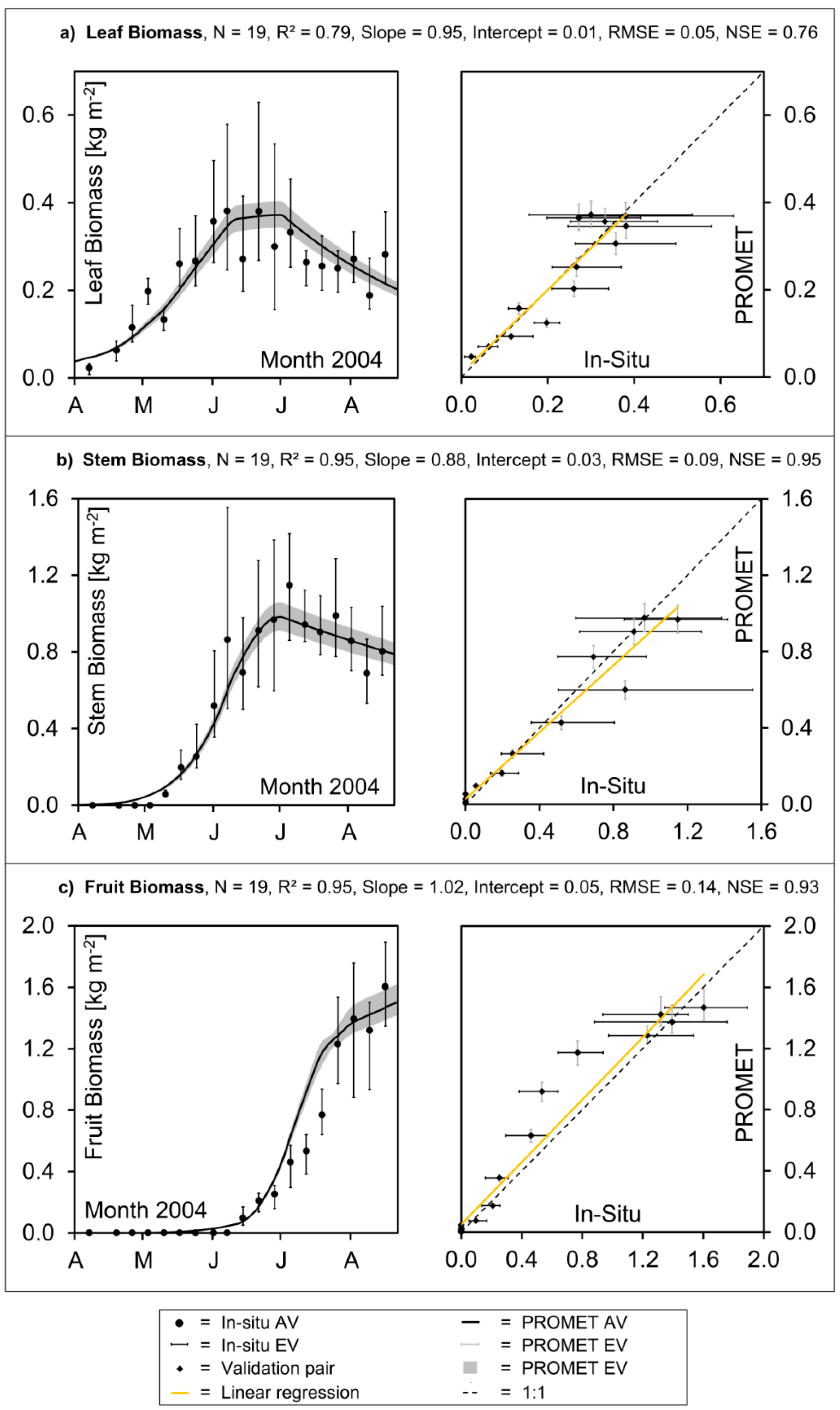
Remotesensing 07 03934 g005
Figure 6. Validation of aboveground dry biomass accumulation of winter wheat in southern Germany: Modelled values vs. in situ measurements: (a) leaf biomass, (b) stem biomass, (c) fruit biomass.
Remotesensing 07 03934 g006
The rapid increase of the leaf area in spring, the peak around the middle of June as well as the steady decrease during the ripening phase is well reproduced by the model. The modelled decrease of leaf area during July is steeper compared to the measurements (Figure 5a, left). This is due to the fact that the non-destructive field measurements represent the total plant area, while the model actually calculates the photosynthetically active LAI (greenLAI), which is characterized by the decomposition of chlorophyll pigments during senescence. From the 16 available measurements of LAI only the 10 dates that were measured before the crop had developed to the phenological stage of fruit development (BBCH stage 70) are included in the validation plot (Figure 5a, right). Nonetheless, the spatial variation of both, the measured and the modelled values, has the same dimension of roughly one LAI unit during the summer months.
The height of the modelled canopy largely influences the energy balance of the leaf because the height of the plants determines the advection of air into the canopy. For winter wheat, the canopy height is modelled as a direct function of the LAI, applying a crop-specific ratio between LAI and canopy height (LHrel in Table 1). Compared to the measured data, the modelled canopy height develops approximately one week earlier, but the height of the fully developed canopy is closely met by the model (Figure 5b, left).
The most determining factor, concerning the realistic representation of the carbon allocation to the different fractions of the canopy, is a correct representation of phenological progress. The simulation of phenological progress is mainly determined through the air temperature. The realistic representation of the air temperature through the spatial interpolation of meteorological station data consequently leads to a rather precise mapping of the phenological stages (Figure 5c). Figure 5c also indicates that the process of hibernation is well traced by the model, as well as the rapid phenological development that characterizes the month of June. For the aboveground canopy fractions of “leaf”, “stem” and “fruit,” the modelled values of dry biomass reasonably match the field data concerning magnitude and seasonal development (Figure 6a–c).
While the average accumulation of leaf mass and leaf senescence is generally traced, the high heterogeneity of the measurements is not reproduced by the model (Figure 6a). Both a large spatial heterogeneity of the measured data and a strong scattering of the average values can be observed. This clearly reveals the measured data to be the result of destructive measuring techniques (see Section 2.4), manifested in jumps and steps that are most prominent in the in situ data of leaf biomass (Figure 6a) and lowest for the fruit dry weight (Figure 6c). The rapid increase of the stem dry weight during the stem elongation phase is well reproduced by the model, while the maximum stem mass might be slightly underestimated (Figure 6b, left).
Apart from some deviations, the model results for the three discerned canopy fractions of winter wheat are mostly within the variability range of the in situ measurements. The accurate representation of the magnitude and course of biomass accumulation during the growing season results in high model efficiency indices, with Nash-Sutcliffe coefficients varying between 0.79 for the leaves (Figure 6a, right), 0.93 for the fruit (Figure 6c, right) and 0.97 for the weight of the stems (Figure 6b, right). In addition, the regressions mostly stay close to the one-to-one line and the respective intercepts are low, both indicating a non-biased representation of the biomass development through the model.
Altogether, the spatially distributed modeling of photosynthesis controlled vegetation growth with PROMET shows high correlations concerning R2, RMSE as well as Nash-Sutcliffe coefficients for all of the observed variables. The good representation of the phenological progress contributes to a realistic simulation of assimilate allocation into aboveground canopy fractions for the C3 metabolism winter crop and thus potentially allows for the delineation of crop yield from the fruit biomass. However, the models’ ability to reproduce spatial heterogeneities is limited by the spatial detail of the input parameters, so that the modelled variability, without remote sensing input, stays behind the variability observed in the field.

3.3. Validation of Spatial Dynamics

For the validation of the models capacity of reproducing spatial growth patterns based on the temporally highly resolved processes, the model was set up for the test site in northern Germany at a spatial resolution of 20 m. The spatial resolution thereby meets the information needs of farmers, because the machinery currently used for site-specific applications to the knowledge of the authors operates at spatial units between 24 and 36 m. The required spatial inputs (digital terrain model, soil map) were derived from publicly available data sources, while the meteorological driver variables were acquired from a met-service. The geometric features of the modelled fields as well as the dates of sowing and harvest could be derived from the Farm Management Information Systems (FMIS) of the test farms (Table 4).
Table 4. Basic input parameters used for the setup of the PROMET model for the test site in Northern Germany at a spatial resolution of 20 m.
Data SetData SourceYearResolution
Soil MapHarmonized World Soil Database (HWSD, [69])200930 arcsec
Digital Terrain ModelShuttle Radar Topography Mission (SRTM, [70])200890 m
Farm MaskFarm Management Information System (FMIS)2010/201120 m
Meteorologymet-service2009–201110 stations (1 hour)
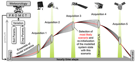
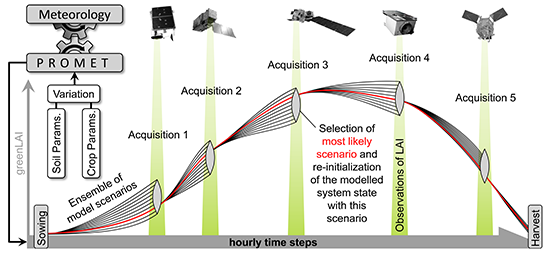
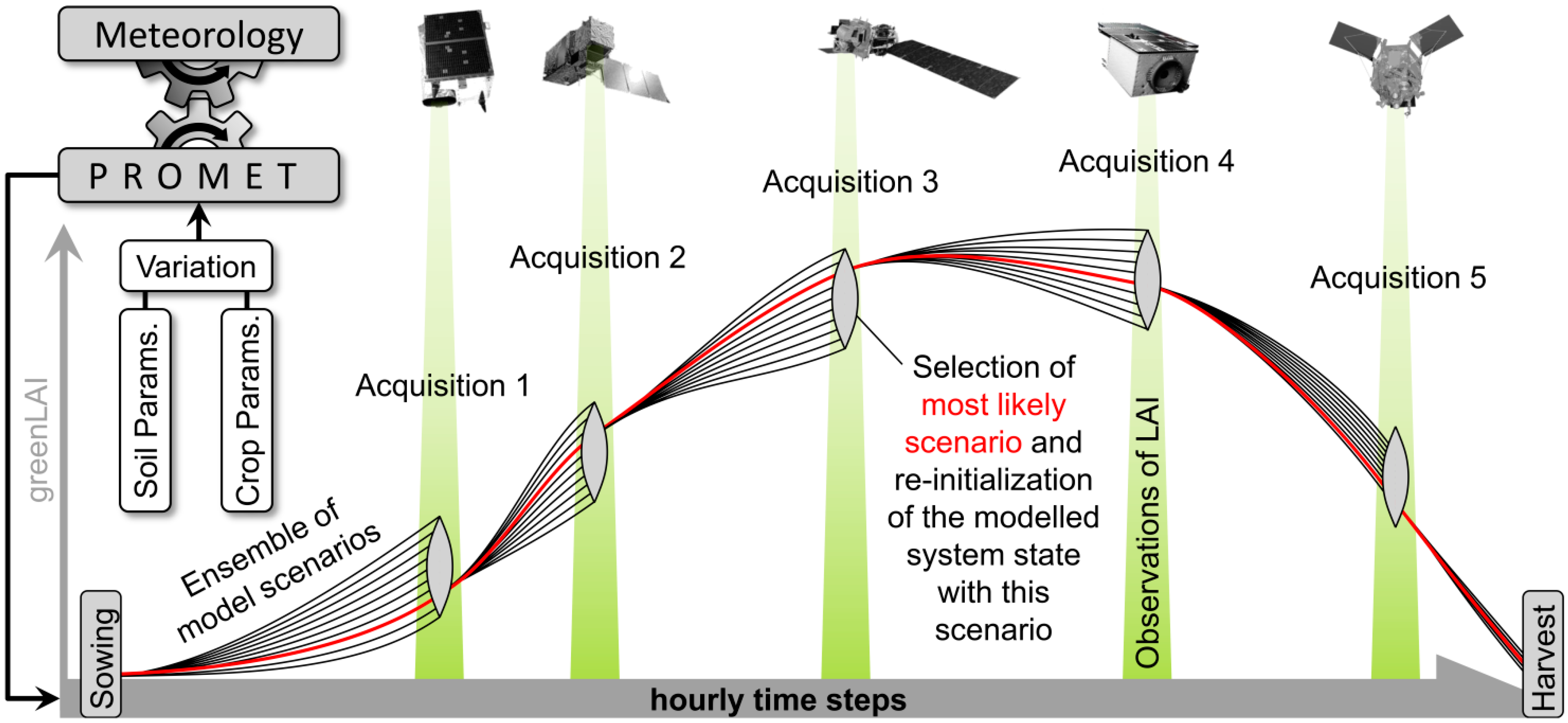
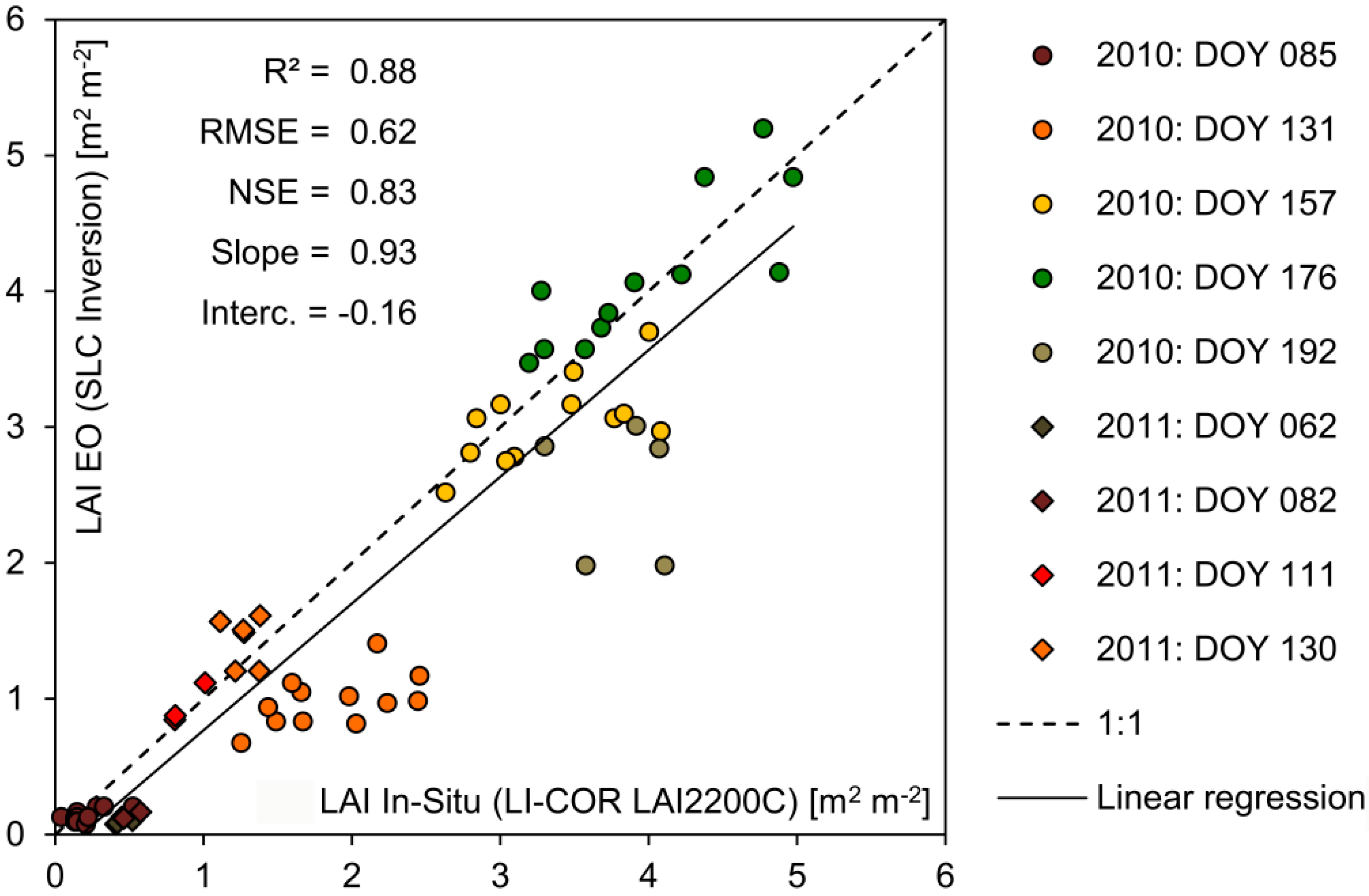
Because the assimilation algorithm relies on multiple observations during the course of one growing season (see Section 2.3), multi-sensoral inputs should be taken into account to increase the probability of data availability. Spatially explicit maps of photosynthetically active leaf area could be derived from satellite images by applying model inversion techniques based on the complex canopy reflectance model SLC (Soil-Leaf-Canopy) [61,62]. A total of five image acquisitions were available for 2010 and seven images for 2011 (Table 5). All spatial inputs including the greenLAI maps from both sensors were resampled to the common 20 m information unit and geometrically referenced to the model environment.
Table 5. Earth Observation data available for assimilation into the PROMET model (OZA = Observer Zenith Angle, GSD = Ground Sampling Distance, RE = RapidEye, TM = Landsat 5 TM).
Date 2010May 21stJun 16thJun 29thJul 8thJul 20th
SensorRERETMTMRE
OZA [°]10.336.96NadirNadir−12.04
GSD [m]5530305
Date 2011Mar 3rdApr 2ndApr 18thMay 5thJun 2ndJun 29thJul 27th
SensorRERERERERERETM
OZA [°]−19.553.606.736.990.34−6.18Nadir
GSD [m]55555530
Taking the models’ good performance with respect to the reproduction of subdivided aboveground biomass accumulation into account (see Section 3.2), the biomass values modelled for the fruit fraction of the canopy were considered as yield, after they had been reduced by a factor of 0.73 (Table 1), accounting for dead material such as husks etc., which contributes to the fruit biomass but is not part of the actual grain yield. The value of this factor is based on [71], who have observed chaff contents of 27% for a selection of common wheat varieties. Being operated in ensemble mode (see Section 2.3), the PROMET model was used to integrate the spatial heterogeneity imprinted in the greenLAI signal of the satellite observations into the modelled biomass and yield values. The resulting modelled spatial yield maps show high agreement with the spatial yield measurements for the two investigated seasons with respect to average, variability, standard deviation and spatial patterns (Table 6). 
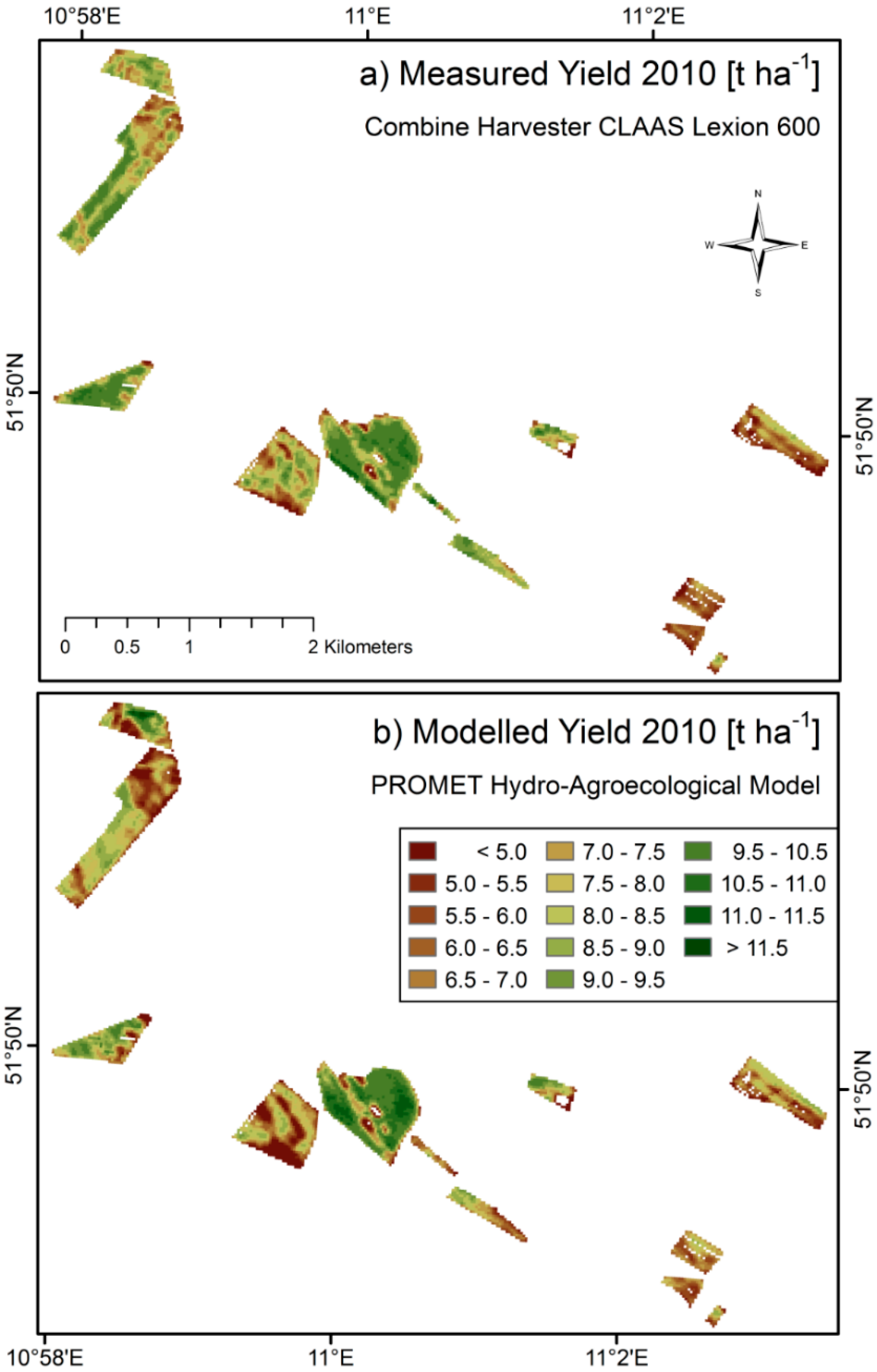
Figure 7 directly compares the measured and modelled yield maps obtained for the season of 2010. Due to reasons of better comparability, the modelled yield map is masked to the pixels, where in situ measurements were available. Data gaps within the fields are due to failures in the combine harvester yield measuring system. The model is able to produce spatially continuous gap-free yield maps.
Figure 7. Spatial comparison of measured (a) and modelled (b) yield of winter wheat fields from the harvesting season of 2010 in northern Germany. Both maps are calculated for a spatial resolution of 20 × 20 m. The surface area of the displayed winter wheat fields amounts to >180 ha. A quantitative comparison is given in Figure 8 and Table 6.
Remotesensing 07 03934 g007
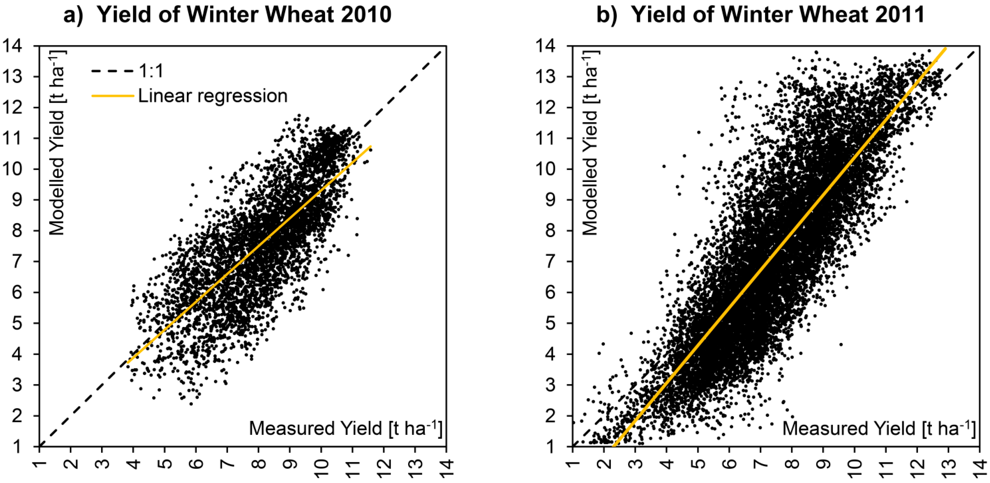
The visual comparison is supported by a direct correlation of measured and modelled spatial data, which is displayed in Figure 8 for both respected seasons. Due to the fact that the area considered for the year 2011 is nearly three times larger as the area modelled for 2010, it is not surprising that the overall heterogeneity was higher for 2011 (Table 6). Although modelled and measured yield maps show a positive correlation for both seasons, a quite high amount of scattering still can be observed. Interpreting the scatterplots in Figure 8, it has to be taken into account that the data clouds are the result of the comparison of two spatial data sets, so that not only thematic but also geometric distortions may contribute to the overall error.
Figure 8. X-Y-Plots showing the correlation of modelled vs. measured yield of all winter wheat pixels for the two consecutive seasons of 2010 (a) and 2011 (b). The corresponding statistics are given in Table 6.
Remotesensing 07 03934 g008
Table 6. Statistics of the validation of winter wheat yield for the two consecutive seasons of 2010 and 2011 corresponding to the X-Y-plots displayed in Figure 8.
IndicatorSymbol20102011
Population:N [pixels]456013135
Area:A [ha]182.4525.4
Coefficient of Determination:R² [–]0.580.70
Slope of linear regression:α [–]0.901.22
Intercept of linear regression:β [t∙ha-1]0.271.81
Root Mean Square Error:RMSE [t∙ha−1]1.291.59
Nash−Sutcliffe Coefficient of Model Efficiency:NSE [–]0.500.67
Average Measured Yield:Ø Meas. [t∙ha−1]8.127.42
Average Modelled Yield:Ø Mod. [t∙ha−1]7.617.23
Standard Deviation Measured Yield:σ Meas. [t∙ha−1]1.531.92
Standard Deviation Modelled Yield:σ Mod. [t∙ha−1]1.812.79
Minimum Measured Yield:Min. Meas. [t∙ha−1]3.830.90
Minimum Modelled Yield:Min. Mod. [t∙ha−1]2.391.11
Maximum Measured Yield:Max. Meas. [t∙ha−1]11.5812.90
Maximum Modelled Yield:Max. Mod. [t∙ha−1]11.7414.58
The direct comparison of the statistics of both seasons is difficult, mostly because the locations of fields cultivated with winter wheat differ between the years. Crop rotation in the test area normally replaces winter wheat with rapeseed; in very few cases a crop rotation system with two consecutive seasons of wheat cultivation was applied. Field 33 is one example (Figure 9 and Figure 10), where winter wheat was cultivated during both respected seasons. Field 33 thus allows for a direct comparison of the two seasons and enables a view on the model’s capacity of also tracing distinct variations between different growth years.
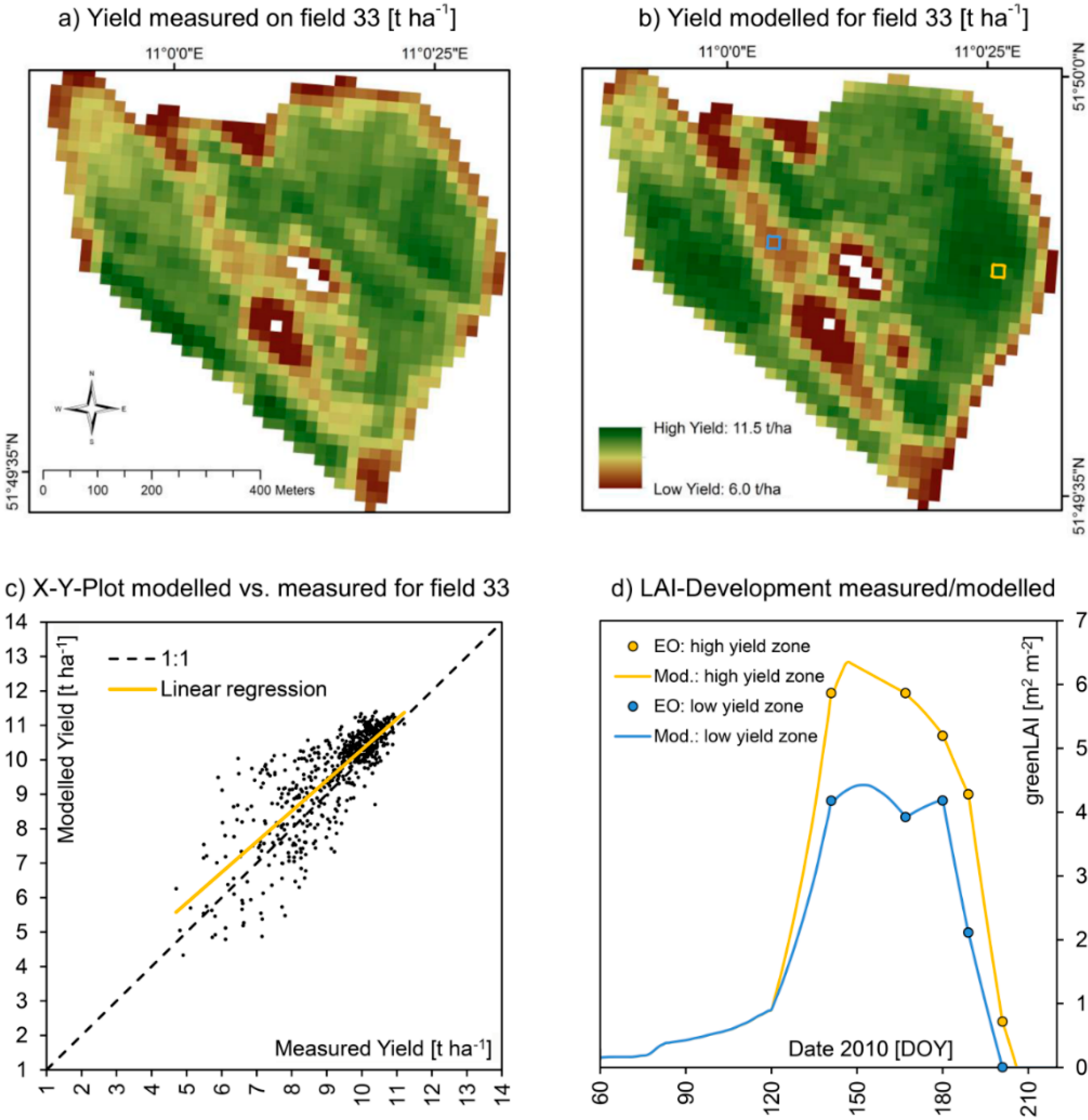
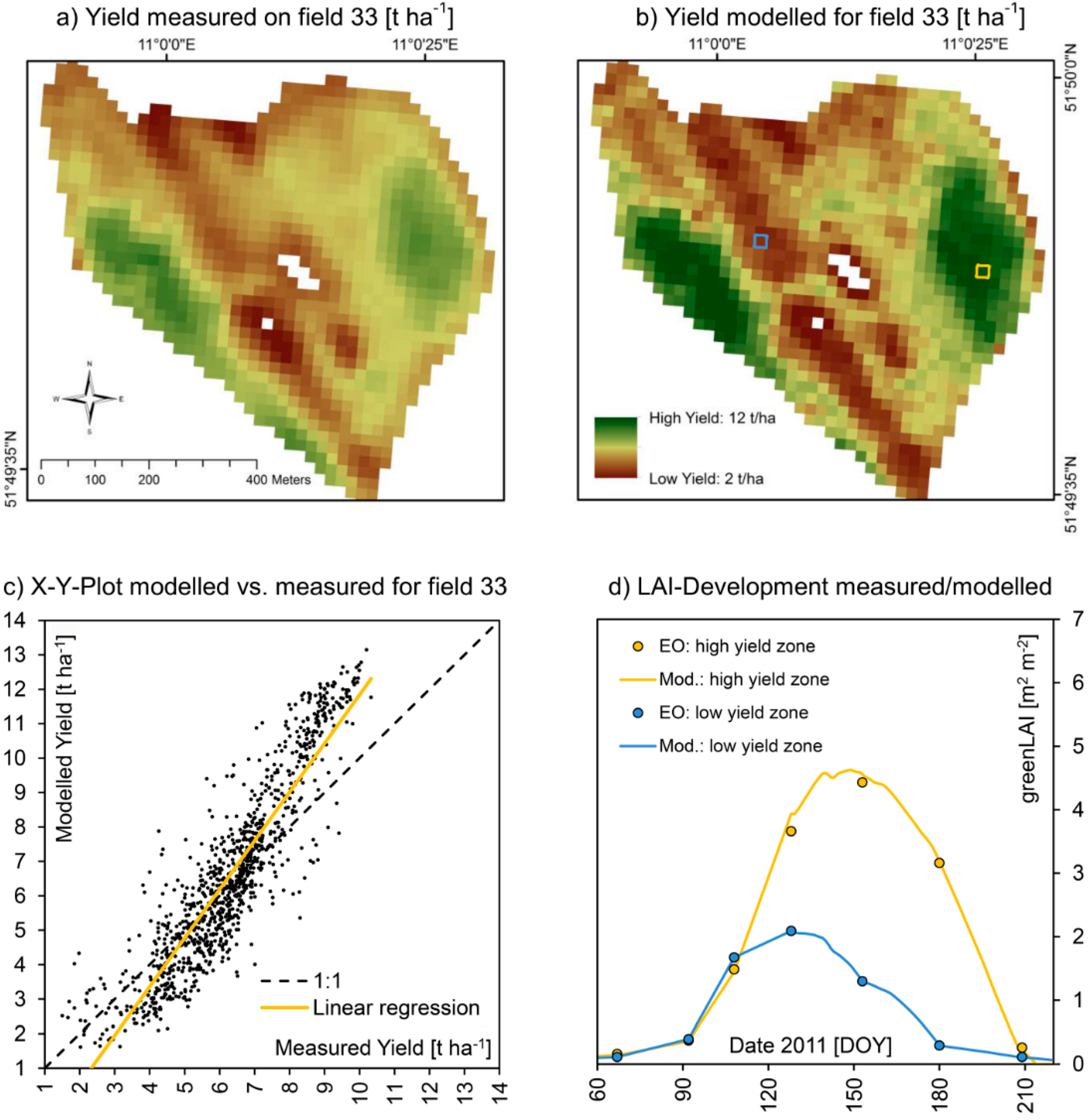
Figure 9. (a) Zoom image from Figure 7, showing spatially measured (a) and modelled (b) yield of winter wheat on test field 33 for the harvesting season of 2010, including an X-Y-plot of the correlation of the two spatial datasets (c) as well as the modelled and EO-measured seasonal course of LAI-development for high (yellow pixel) and low (blue pixel) yielding sections of the field (d). A quantitative comparison is given in Table 7.
Remotesensing 07 03934 g009
Figure 9 and Figure 10 show a detailed view of the approximately 40 ha large field and compare measured and modelled values for both seasons. With 9.26 t∙ha−1, the average yield of field 33 in 2010 was significantly higher compared to 2011 where only 6.29 t∙ha−1 were harvested, while the spatial heterogeneity was higher in 2011 compared to 2010, standard deviation increasing from 1.3 to 1.7 t∙ha−1. This mostly can be traced to a strong scarcity of rainfall during the summer of 2011, resulting in phases of drought especially during May and June 2011. While during the growth cycle of 2010 about 563 mm of precipitation were registered at the test field, in 2011 only 476 mm of rainfall were measured. Under drought conditions, small-scale variations of soil quality become more distinctly visible in the yield map, resulting in a higher difference between low and high yielding sections of the field. For the more favorable growth conditions of 2010, the model was perfectly able to reproduce the measured yield map. For the more extreme meteorological conditions of 2011, the model performed equally well, but tended to overestimate high yielding field sections more distinctly compared to 2010 (Table 7). The spatial patterns are nonetheless well reproduced by the model also for 2011, resulting in a high coefficient of determination of 0.82.
Figure 10. Spatially measured (a) and modelled (b) yield of winter wheat on test field 33 for the harvesting season of 2011, including an X-Y-plot of the correlation of the two spatial datasets (c) as well as the modelled and EO-measured seasonal course of LAI-development for high (yellow pixel) and low (blue pixel) yielding sections of the field (d). A quantitative comparison is given in Table 7.
Remotesensing 07 03934 g010
Table 7. Validation statistics for field 33 (2010 vs. 2011). Also compare Figure 9 and Figure 10.
Indicator 20102011
N=1019 [Pixels]1019 [pixels]
A=40.76 [ha] 40.76 [ha]
=0.67 [–]0.82 [–]
α=0.89 [–]1.41 [–]
β=1.39 [t∙ha-1]−2.3 [t∙ha-1]
RMSE=0.92 [t∙ha-1] 1.38 [t∙ha-1]
NSE =0.53 [–]0.34 [–]
Ø Meas. / Mod.=9.16/9.54 [t∙ha−1] 6.29/6.59 [t∙ha−1]
σ Meas. / Mod.=1.30/1.42 [t∙ha−1] 1.70/2.66 [t∙ha−1]
Min. Meas. / Mod. =4.70/4.33 [t∙ha−1] 1.50/1.62 [t∙ha−1]
Max. Meas. / Mod.=11.21/11.40 [t∙ha−1]10.33/13.15 [t∙ha−1]

4. Conclusions

The enhanced hydro-agroecological model PROMET enables the temporally and spatially explicit simulation of crop growth at the field scale. The seasonal development of structural canopy variables as well as the corresponding fractionized biomass accumulation could successfully be validated for a C3 metabolism winter crop using measured sample point data obtained from a field campaign. The model results show high agreement for the aboveground plant fractions leaf, stem and fruit. However, the spatial heterogeneity of the field scale, as indicated by the field measurements, could not fully be traced by the model without assimilating remote sensing data. The relatively homogeneous stand-alone model results indicate that the model is ignorant of certain spatial information. The spatial patterns observed without help of additional information by EO are mainly caused by variations of illumination, temperature and radiation budget in dependence of the terrain situation (elevation, slope, aspect), which again affect the photosynthetic productivity. Besides those terrain-induced conditions, the spatial distribution of soil parameters influences modelled plant growth through the spatially differentiated water and nutrient supply. It is clear that these soil patterns could not be adequately captured with the available soil maps without EO data assimilation.
In order to bridge the problem of underestimated spatial heterogeneity for field-scale applications, the ensemble-based assimilation of remote sensing data was successfully integrated. It enables the simulation of realistic yield maps of agricultural sites including in-field heterogeneities. Agreements are very high, both in terms of absolute values and spatial patterns. Even pixel-wise comparisons between simulated yield maps and interpolated combine harvester measurements correlate significantly.
The concept of using EO-based information for crop growth simulations have been well recognized by the remote sensing community. The synergistic combination of remote sensing data and process-based model also allows simulating crop variables that cannot directly be measured with an optical sensor. Despite the potential of this method, it also has its limitations. For example, the need of various input/parameter data for models as well as tedious calibrations could hamper the operational applications. Accordingly we avoided site-specific calibration and used physical-based, transferable approaches. The overall data efficiency (i.e., the ratio of the amount of data and information needed for implementation of the approach to the improvement of output information) is another important criterion for the selection of the most suitable approach. This was analyzed in an earlier study [72] and showed that four acquisitions well distributed over the crop-growing period are necessary for high quality results. Additional scenes only slightly improved the model performance.
The explicit spatial validation of in-field patterns is one of the major achievements of this study compared to other recent approaches in the field of remote sensing supported yield modeling, e.g., [28,64,73]. While other studies (e.g., [63] and [21]) use simulated and observed soil-adjusted vegetation indices for the assimilation, in our approach the greenLAI is used as common variable between model and observation. It is retrieved using a canopy reflectance model, taking illumination geometry and background signal into account. The assimilation, however, neglects possible errors, which applies to the crop growth model side as well as to the remote sensing side. The results of both are taken into account with full confidence. For example, all scenarios of the ensemble are considered with the same probability. Ensemble Kalman filtering, as e.g., proposed by [24], or particle filtering, as e.g., applied by [64], is not yet part of the assimilation procedure. Although the results achieved with this method are very accurate, they largely depend on the quality of the greenLAI retrieval. Errors in these retrievals directly affect the accuracy of modelled yield. In a next step, the integration of levels of confidence on both sides will be investigated. Uncertainties thus could be taken into account in the assimilation process to further improve the performance. The spatial patterns that were derived with help of the model can be assumed to be mainly caused by varying soil quality. Other influences might e.g., be the occurrence of mechanical stress or of pests and diseases. The applied technique, being based on the detection of growth deviations from the expected development of the field, does not directly allow for a differentiation of reasons. The differentiation of short-term growth influencing conditions from long-term soil characteristics may, however, be possible by analyzing the multiyear recurrence of growth patterns. This is a topic of future research. It will have to consider that some soil patterns, such as water-holding capacity, may only be visible in years with water scarcity.
The proposed ensemble-based assimilation technique nonetheless allows for the generation of continuous spatiotemporal model results on biomass and yield on farm and regional level. These results are temporally and spatially highly correlated with dynamic and non-linear crop growth observed in the field. Conventional yield maps from combine harvesters only provide destructive spatial measurements at harvest and thus cannot be applied during the growing season. The information that may be drawn from remote sensing-supported model results on an hourly basis for the entire course of an agricultural growing season forms a solid basis for site-specific management decisions. These again are prerequisites for efficient and sustainable agriculture.

Acknowledgments

The research presented in this article was conducted at the Chair of Geography and Remote Sensing, Department of Geography, Ludwig-Maximilians-Universität Munich in close cooperation with VISTA Remote Sensing in Geosciences GmbH Munich. The enhancement of the PROMET model was supported by the German Research Foundation (DFG) in the frame of the project “Coupled Analysis of Vegetation Chlorophyll and Water Content Using Hyperspectral, Bidirectional Remote Sensing” (Grant Number: OP 92/1-1/2) as well as through the joint project “GLOWA Danube—Global Change and the Hydrological Cycle” (Grant number: 01LW0602A2), funded by the German Federal Ministry of Education and Research (BMB+F). The concept of remote sensing data assimilation was initially developed in the Project “RapidSAR-Integrative use of RapidEye and TerraSAR-X through data assimilation into models of agricultural production,” supported by DLR/BMWi under the grant code numbers 50 EE 0920 and 50 EE 0922. Validation in the northern Germany test site was conducted within the project “TalkingFields,” funded by the ESA ARTES 20 Integrated Application Promotion program under contract 4000100879/10/NL/US. The authors would like to thank the agricultural holdings in the different test areas for the supply of validation data. RapidEye data was provided via the RapidEye Science Archive (RESA) operated by DLR Neustrelitz, Germany.

Author Contributions

Tobias B. Hank is assistant professor at the Department of Geography of the LMU Munich, Germany. He integrated the biophysical components into the PROMET model, carried out the demonstrations and validations and did the major part of the preparation of the manuscript. Heike Bach is the managing director of VISTA Remote Sensing in Geosciences GmbH, a value adding company located in Munich, Germany. She was involved in the development of the canopy reflectance model SLC, carried out the EO analyses, the derivation of greenLAI and contributed to the preparation of the manuscript. Wolfram Mauser is full professor at the Department of Geography of the LMU Munich and leader of the remote sensing research group. He has been developing the hydrological model PROMET for more than 20 years and has assisted with the preparation of this manuscript. The data assimilation concept was developed by all three authors.

Conflicts of Interest

The authors declare no conflict of interest.

References

  1. Auernhammer, H. Precision farming—The environmental challenge. Comput. Electron. Agr. 2001, 30, 31–43. [Google Scholar] [CrossRef]
  2. Delgado, J.A.; Khosla, R.; Mueller, T. Recent advances in precision (target) conservation. J. Soil Water Conserv. 2011, 66, 167A–170A. [Google Scholar] [CrossRef]
  3. Dobermann, A.; Blackmore, S.; Cook, S. E.; Adamchuk, V. I. Precision farming: Challenges and future directions. Available online: http://scholar.google.com.tw/scholar?q=Precision+farming%3A+Challenges+and+future+directions&btnG=&hl=zh-TW&as_sdt=0%2C5 (accessed on 30 September 2014).
  4. Van Lynden, G.W.J.; Mantel, S. The role of GIS and remote sensing in land degradation assessment and conservation mapping: Some user experiences and expectations. Int. J. Appl. Earth Obs. Geoinf. 2001, 3, 61–68. [Google Scholar] [CrossRef]
  5. Verhoef, W.; Bach, H. Simulation of hyperspectral and directional radiance images using coupled biophysical and atmospheric radiative transfer models. Remote Sens. Environ. 2003, 87, 23–41. [Google Scholar] [CrossRef]
  6. Bach, H.; Friese, M.; Spannraft, K.; Migdall, S.; Dotzler, S.; Hank, T.; Mauser, W. Integrative use of multitemporal RapidEye and Terrasar-X data for agricultural monitoring. In Proceedings of IEEE International Geoscience and Remo2te Sensing Symposium IGARSS, Munich, Germany, 22–27 July 2012.
  7. Lu, D. The potential and challenge of remote sensing-based biomass estimation. Int. J. Remote Sens. 2006, 27, 1297–1328. [Google Scholar] [CrossRef]
  8. Foley, J.A. An integrated biosphere model of land surface processes, terrestrial carbon balance, and vegetation dynamics. Glob. Biogeochem. Cy. 1996, 10, 603–628. [Google Scholar] [CrossRef]
  9. Sitch, S.; Smith, B.; Prentice, I.C.; Arneth, A.; Bondeau, A.; Cramer, W.; Venevsky, S. Evaluation of ecosystem dynamics, plant geography and terrestrial carbon cycling in the LPJ dynamic global vegetation model. Glob. Change Biol. 2003, 9, 161–185. [Google Scholar] [CrossRef]
  10. Bachelet, D. MC1: A Dynamic Vegetation Model for Estimating The Distribution of Vegetation and Associated Ecosystem Fluxes of Carbon, Nutrients and Water; DIANE Publishing: Darby, PA, USA, 2001. [Google Scholar]
  11. Jones, J. W.; Hoogenboom, G.; Porter, C.H.; Boote, K.J.; Batchelor, W.D.; Hunt, L.A.; Ritchie, J.T. The DSSAT cropping system model. Eur. J. Agron. 2003, 18, 235–265. [Google Scholar] [CrossRef]
  12. Yin, X.; van Laar, H.H. Crop Systems Dynamics: An Ecophysiological Model of Genotype-by-Environment Interactions (GECROS); Wageningen Academic Publishers: Wageningen, The Netherlands, 2005. [Google Scholar]
  13. Diepen, C.V.; Wolf, J.; Keulen, H.V.; Rappoldt, C. Wofost—A simulation-model of crop production. Soil Use Manag. 1989, 5, 16–24. [Google Scholar] [CrossRef]
  14. Lindström, G.; Johansson, B.; Persson, M.; Gardelin, M.; Bergström, S. Development and test of the distributed HBV-96 hydrological model. J. Hydrol. 1997, 201, 272–288. [Google Scholar] [CrossRef]
  15. Refsgaard, J.C.; Storm, B. MIKE SHE. Available online: http://www.cabdirect.org/abstracts/19961904783.html;jsessionid=E6E50730DC54EBDD10C739B063F3E64F (accessed on 30 September 2014).
  16. Arnold, J.G.; Allen, P.M.; Bernhardt, G. A comprehensive surface-groundwater flow model. J. Hydrol. 1993, 142, 47–69. [Google Scholar] [CrossRef]
  17. Beven, K.J.; Quinn, P.; Romanowicz, R.; Freer, J.; Fisher, J.; Lamb, R. TOPMODEL and GRIDATB, A Users Guide to the Distribution Versions (94.01); Technical Report TR110/94; Lancaster University Centre For Research On Environmental Systems and Statistics: Lancaster, England, 1994. [Google Scholar]
  18. Lohmann, D.; Raschke, E.; Nijssen, B.; Lettenmaier, D.P. Regional scale hydrology: I. Formulation of the VIC-2L model coupled to a routing model. Hydrol.Sci. J. 1998, 43, 131–141. [Google Scholar] [CrossRef]
  19. Benoit, R.; Pellerin, P.; Kouwen, N.; Ritchie, H.; Donaldson, N.; Joe, P.; Soulis, E.D. Toward the use of coupled atmospheric and hydrologic models at regional scale. Mon. Weather Rev. 2000, 128, 1681–1706. [Google Scholar] [CrossRef]
  20. Mauser, W.; Bach, H. PROMET—Large scale distributed hydrological modelling to study the impact of climate change on the water flows of mountain watersheds. J. Hydrol. 2009, 376, 362–377. [Google Scholar] [CrossRef]
  21. Launay, M.; Guerif, M. Assimilating remote sensing data into a crop model to improve predictive performance for spatial applications. Agr. Ecosyst. Environ. 2005, 111, 321–339. [Google Scholar] [CrossRef]
  22. Bouman, B. Crop modelling and remote sensing for yield prediction. NJAS Wageningen J. Life Sci. 1995, 43, 143–161. [Google Scholar]
  23. Bach, H. Yield estimation of corn based on multitemporal Landsat-TM data as input for an agrometeorological model. J. Eur. Opt. Soc. Part A 1998, 7. [Google Scholar] [CrossRef]
  24. Dorigo, W.A.; Zurita-Milla, R.; de Wit, A.J.; Brazile, J.; Singh, R.; Schaepman, M.E. A review on reflective remote sensing and data assimilation techniques for enhanced agroecosystem modeling. Int. J. Appl. Earth Obs. Geoinf. 2007, 9, 165–193. [Google Scholar] [CrossRef]
  25. Vazifedoust, M.; van Dam, J.C.; Bastiaanssen, W.G.M.; Feddes, R.A. Assimilation of satellite data into agrohydrological models to improve crop yield forecasts. Int. J. Remote Sens. 2009, 30, 2523–2545. [Google Scholar] [CrossRef]
  26. De Wit, A.; Duveiller, G.; Defourny, P. Estimating regional winter wheat yield with WOFOST through the assimilation of green area index retrieved from MODIS observations. Agr. Forest Meteorol. 2012, 164, 39–52. [Google Scholar]
  27. Dente, L.; Satalino, G.; Mattia, F.; Rinaldi, M. Assimilation of leaf area index derived from ASAR and MERIS data into CERES-Wheat model to map wheat yield. Remote Sens. Environ. 2008, 112, 1395–1407. [Google Scholar] [CrossRef]
  28. Li, Y.; Zhou, Q.; Zhou, J.; Zhang, G.; Chen, C.; Wang, J. Assimilating remote sensing information into a coupled hydrology-crop growth model to estimate regional maize yield in arid regions. Ecol. Model. 2014, 291, 15–27. [Google Scholar] [CrossRef]
  29. Panda, S.S.; Ames, D.P.; Panigrahi, S. Application of vegetation indices for agricultural crop yield prediction using neural network techniques. Remote Sens. 2010, 2, 673–696. [Google Scholar] [CrossRef]
  30. IUSS-Working-Group-WRB. World Reference Base for Soil Resources 2006. Available online: http://url/?q=ftp://ftp.fao.org/agl/agll/docs/wsrr103e.pdf (accessed on 30 September 2014).
  31. Farquhar, G.D.; Caemmerer, S.; Berry, J.A. A biochemical model of photosynthetic CO2 assimilation in leaves of C3 species. Planta 1980, 149, 78–90. [Google Scholar] [CrossRef] [PubMed]
  32. Chen, D.-X. Mathematical simulation of C4 grass photosynthesis in ambient and elevated CO2. Ecol. Model. 1994, 73, 63–80. [Google Scholar] [CrossRef]
  33. Hodges, T.; Ritchie, J.T. The CERES-Wheat phenology model. In Predicting Crop Phenology; CRC Press: Boston, MA, USA, 1991; pp. 133–142. [Google Scholar]
  34. Jones, C.; Kiniry, J.R. CERES-Maize—A Simulation Model of Maize Growth and Development; Texas A&M University Press: Michigan, MI, USA, 1986. [Google Scholar]
  35. Hank, T.B. A Biophysically Based Coupled Model Approach for the Assessment of Canopy Processes under Climate Change Conditions. Available online: http://edoc.ub.uni-muenchen.de/8725/ (accessed on 30 September 2014).
  36. Richards, L.A. Capillary conduction of liquids through porous mediums. J. Appl. Phys. 1931, 1, 318–333. [Google Scholar]
  37. Mauser, W.; Schädlich, S. Modelling the spatial distribution of evapotranspiration on different scales using remote sensing data. J. Hydrol. 1998, 212–213, 250–267. [Google Scholar] [CrossRef]
  38. Ludwig, R.; Mauser, W. Modelling catchment hydrology within a GIS based SVAT-model framework. Hydrol. Earth Syst. Sci. 1999, 4, 239–249. [Google Scholar] [CrossRef]
  39. Strasser, U.; Mauser, W. Modelling the spatial and temporal variations of the water balance for the Weser catchment 1965–1994. J. Hydrol. 2001, 254, 199–214. [Google Scholar] [CrossRef]
  40. Prasch, M.; Mauser, W.; Weber, M. Quantifying present and future glacier melt-water contribution to runoff in a central Himalayan river basin. Cryosphere 2013, 7, 889–904. [Google Scholar] [CrossRef]
  41. Zabel, F.; Mauser, W. 2-Way coupling the hydrological land surface model PROMET with the regional climate model MM5. Hydrol. Earth Syst. Sci. 2013, 17, 1705–1714. [Google Scholar] [CrossRef]
  42. Marke, T.; Mauser, W.; Pfeiffer, A.; Zängl, G.; Jacob, D.; Strasser, U. Application of a hydrometeorological model chain to investigate the effect of global boundaries and downscaling on simulated river discharge. Environ. Earth Sci. 2014, 71, 4849–4868. [Google Scholar] [CrossRef]
  43. Friend, A.D.; Stevens, A.K.; Knox, R.G.; Cannell, M.G.R. A process-based, terrestrial biosphere model of ecosystem dynamics (Hybrid v3.0). Ecol. Model. 1997, 95, 249–287. [Google Scholar] [CrossRef]
  44. Farquhar, G.D.; von Caemmerer, S.; Berry, J.A. Models of photosynthesis. Plant Physiol. 2001, 125, 42–45. [Google Scholar] [CrossRef] [PubMed]
  45. Aphalo, P.J.; Jarvis, P.G. Do stomata respond to relative humidity? Plant Cell Environ. 1991, 14, 127–132. [Google Scholar] [CrossRef]
  46. Medlyn, B.E.; Dreyer, E.; Ellsworth, D.; Forstreuter, M.; Harley, P.C.; Kirschbaum, M.U.F.; Loustau, D. Temperature response of parameters of a biochemically based model of photosynthesis. II. A review of experimental data. Plant Cell Environ. 2002, 25, 1167–1179. [Google Scholar] [CrossRef]
  47. Wu, A.; Black, A.; Verseghy, D.L.; Bailey, W.G. Comparison of two-layer and single-layer canopy models with Lagrangian and K-theory approaches in modelling evaporation from forests. Int. J. Climatol. 2001, 21, 1821–1839. [Google Scholar] [CrossRef]
  48. Campbell, G.S. Extinction coefficients for radiation in plant canopies calculated using an ellipsoidal inclination angle distribution. Agr. Forest Meteorol. 1986, 36, 317–321. [Google Scholar] [CrossRef]
  49. Nobel, P.S. Physiochemical and Environmental Plant Physiology; Elsevier Academic Press: Burlington, ON, USA, 2005. [Google Scholar]
  50. Cionco, R.M. A mathematical model for air flow in a vegetative canopy. J. Appl. Meteorol. 1965, 4, 517–522. [Google Scholar] [CrossRef]
  51. Ball, J.T.; Woodrow, I.E.; Berry, J.A. A model predicting stomatal conductance and its contribution to the control of photosynthesis under different environmental conditions. Progress Photosynth. Res. 1987, 4, 221–224. [Google Scholar]
  52. Reichstein, M. Drought Effects on Carbon and Water Exchange in Three Mediterranean Ecosystems; Bayreuther Forum Ökologie: Bayreuth, Germany, 2001. [Google Scholar]
  53. Jarvis, P.G.; Morison, J.I.L. The control of transpiration and photosynthesis by stomata. In Stomatal Physiology; Cambridge University Press: Cambridge, UK, 1981. [Google Scholar]
  54. Meier, U. Growth Stages of Mono- and Dicotyledonous Plants; Federal Biological Research Centre for Agriculture and Forestry: Braunschweig, Germany.
  55. Generation of Continuous Agricultural Information Products Using Multi-Temporal High Resolution Optical Data in A Model Framework—The M4Land Project. Available online: http://seom.esa.int/S2forScience2014/files/05_S2forScience-AgricultureI_KLUG.pdf (accessed on 30 September 2014).
  56. Zarco-Tejada, P.J.; Ustin, S.L.; Whiting, M.L. Temporal and spatial relationships between within-field yield variability in cotton and high-spatial hyperspectral remote sensing imagery. Agron. J. 2005, 97, 641–653. [Google Scholar] [CrossRef]
  57. Klar, C.W.; Fiener, P.; Neuhaus, P.; Lenz-Wiedemann, V.I.S.; Schneider, K. Modelling of soil nitrogen dynamics within the decision support system DANUBIA. Ecol. Model. 2008, 217, 181–196. [Google Scholar] [CrossRef]
  58. Robertson, B.; Beckett, K.; Rampersad, C.; Putih, R. Quantitative geometric calibration & validation of the Rapideye constellation. In Proceedings of IEEE International Geoscience and Remote Sensing Symposium, Cape Town, South Africa, 12–17 July 2009.
  59. Darvishzadeh, R.; Atzberger, C.; Skidmore, A.K. Hyperspectral vegetation indices for estimation of leaf area index. In Proceedings of ISPRS Commission VII Mid-term Symposium, Enschede, the Netherlands, 8–11 May 2006.
  60. Richter, K.; Hank, T.B.; Vuolo, F.; Mauser, W.; D’Urso, G. Optimal exploitation of the Sentinel-2 spectral capabilities for crop leaf area index mapping. Remote Sens. 2012, 4, 561–582. [Google Scholar] [CrossRef] [Green Version]
  61. Verhoef, W.; Bach, H. Simulation of Sentinel-3 images by four-stream surface-atmosphere radiative transfer modeling in the optical and thermal domains. Remote Sens. Environ. 2012, 120, 197–207. [Google Scholar] [CrossRef]
  62. Verhoef, W.; Bach, H. Coupled soil-leaf-canopy and atmosphere radiative transfer modeling to simulate hyperspectral multi-angular surface reflectance and TOA radiance data. Remote Sens. Environ. 2007, 109, 166–182. [Google Scholar] [CrossRef]
  63. Guérif, M.; Duke, C.L. Adjustment procedures of a crop model to the site specific characteristics of soil and crop using remote sensing data assimilation. Agr. Ecosyst. Environ. 2000, 81, 57–69. [Google Scholar] [CrossRef]
  64. Machwitz, M.; Giustarini, L.; Bossung, C.; Frantz, D.; Schlerf, M.; Lilienthal, H.; Udelhoven, T. Enhanced biomass prediction by assimilating satellite data into a crop growth model. Environ. Model. Softw. 2014, 62, 437–453. [Google Scholar] [CrossRef]
  65. Blackmore, S. Remedial correction of yield map data. Precis. Agr. 1999, 1, 53–66. [Google Scholar] [CrossRef]
  66. Nash, J.E.; Sutcliffe, J.V. River flow forecasting through conceptual models part I—A discussion of principles. J. Hydrol. 1970, 10, 282–290. [Google Scholar] [CrossRef]
  67. Richter, K.; Atzberger, C.; Hank, T.B.; Mauser, W. Derivation of biophysical variables from Earth observation data: Validation and statistical measures. J. Appl. Remote Sens. 2012, 6. [Google Scholar] [CrossRef]
  68. Moriasi, D.N.; Arnold, J.G.; van Liew, M.W.; Bingner, R.L.; Harmel, R.D.; Veith, T.L. Model evaluation guidelines for systematic quantification of accuracy in watershed simulations. Trans. Am. Soc. Agr. Biol. Eng. 2007, 50, 885–900. [Google Scholar]
  69. FAO. Harmonized World Soil Database (Version 1.21); FAO, IIASA: Rome, Italy and Laxenburg, Austria, 2012. [Google Scholar]
  70. US Geological Survey (USGS). Shuttle Radar Topography Mission, 1 Arc Second Scene, Unfilled Unfinished 2.0. Available online: http://www.landcover.org/data/srtm/ (accessed on 30 September 2014).
  71. Kastelliz, A.; Ruckenbauer, P. Quantifizierung Des Trockenheitsbedingten Ertragsrückganges Bei Getreide Sowie Prüfung der Entwicklung von Verfahren zur Frühzeitigen Prognose Eines Entsprechenden Minderertrages. Available online: https://forschung.boku.ac.at/fis/suchen.publikationen_uni_autoren?sprache_in=en&ansicht_in=&menue_id_in=211&publikation_id_in=18085 (accessed on 30 September 2014).
  72. Hank, T.B.; Frank, T.; Bach, H.; Mauser, W. On the Effect of Multiseasonal Earth Observation Availability for Assimilation-Supported Modelling of Winter Wheat Yield. Available online: http://www.spacebooks-online.com/product_info.php?products_id=17572 (accessed on 30 September 2014).
  73. Zhao, Y.; Chen, S.; Shen, S. Assimilating remote sensing information with crop model using Ensemble Kalman Filter for improving LAI monitoring and yield estimation. Ecol. Model. 2013, 270, 30–42. [Google Scholar] [CrossRef]

