Abstract
Taking advantage of multiple new remote sensing data sources, especially from Chinese satellites, the CropWatch system has expanded the scope of its international analyses through the development of new indicators and an upgraded operational methodology. The approach adopts a hierarchical system covering four spatial levels of detail: global, regional, national (thirty-one key countries including China) and “sub-countries” (for the nine largest countries). The thirty-one countries encompass more that 80% of both production and exports of maize, rice, soybean and wheat. The methodology resorts to climatic and remote sensing indicators at different scales. The global patterns of crop environmental growing conditions are first analyzed with indicators for rainfall, temperature, photosynthetically active radiation (PAR) as well as potential biomass. At the regional scale, the indicators pay more attention to crops and include Vegetation Health Index (VHI), Vegetation Condition Index (VCI), Cropped Arable Land Fraction (CALF) as well as Cropping Intensity (CI). Together, they characterize crop situation, farming intensity and stress. CropWatch carries out detailed crop condition analyses at the national scale with a comprehensive array of variables and indicators. The Normalized Difference Vegetation Index (NDVI), cropped areas and crop conditions are integrated to derive food production estimates. For the nine largest countries, CropWatch zooms into the sub-national units to acquire detailed information on crop condition and production by including new indicators (e.g., Crop type proportion). Based on trend analysis, CropWatch also issues crop production supply outlooks, covering both long-term variations and short-term dynamic changes in key food exporters and importers. The hierarchical approach adopted by CropWatch is the basis of the analyses of climatic and crop conditions assessments published in the quarterly “CropWatch bulletin” which provides accurate and timely information essential to food producers, traders and consumers.
1. Introduction
Food security is one of the most basic factors of our physical and intellectual wellbeing. It is a fundamental prerequisite for a healthy and happy life. Food security is a broad concept that goes beyond production because it requires accounting for spatial and temporal variability of food availability, as well as physical and economic access. Accurate and timely food production information is essential to food producers, traders and consumers.
In order to collect relevant data and to gain firsthand knowledge about the domestic and international agricultural situations, many countries and institutions around the world have developed dedicated agriculture monitoring systems [1] by complementing their traditional ground-based approach with satellite remote sensing based inputs. Their objective is mostly to ensure national food security by shielding domestic market and production from the vagaries of international markets. Such monitoring systems typically operate at different scales, which range from the sub-national, to national and global levels.
At global and regional scales, the Crop Explorer of the U.S. Department of Agriculture (USDA) Foreign Agricultural Service (FAS) is capable of providing near-real time crop condition and agrometeorological monitoring information, and releases monthly global food production estimates [2]. The Global Information and Early Warning System (GIEWS) of the Food and Agriculture Organization (FAO) mainly offers crop monitoring and food supply early warning for developing countries and countries at risk. The Monitoring Agricultural Resources (MARS) Unit of the European Commission (EC), Joint Research Center (JRC) focuses on assessing crop production, farming activities and rural development for European countries. CropWatch, which was developed by the Institute of Remote Sensing and Digital Earth (RADI) in the Chinese Academy of Sciences (CAS), has achieved breakthrough results in the integration of methods, independence of the assessments and support to emergency response by periodically releasing agricultural information for thirty-one countries over the world [1,3].
National monitoring systems caught on after the Sahelian droughts in the 1970s. This includes major food producing countries such as Argentina [4], Brazil [5], Canada [6], and India [7], but also many of the less developed countries on all continents [8,9,10,11,12,13,14]. Some monitoring systems have a thematic focus (e.g., on nutrition: [15]) or adopt a regional approach, such as the AGRHYMET center in West Africa [16].
Many global systems [17,18] are just a simple combination of national systems; they lack any global overview, often remaining descriptive and paying little attention to the driving forces behind abnormal crop conditions. NDVI and FAPAR departures from average conditions are the preferred methodology [2,19,20]. The size differences between countries and the spatial variation of agrometeorological variables within countries are seldom considered; the methodology applied in crop monitoring systems is often obsolete, and production estimation is the main output, which actually provides little early warning information. Both national and global systems are mainly inherited from the Large Area Crop Inventory Experiment (LACIE) of the 1970s, in which production was estimated as the product of yield and area [21,22]. Area was obtained by area sampling with remote sensing while NDVI was used for crop yield estimation, in combination with agrometeorological data [23]. A main factor behind this situation was the limited availability and high cost of remote sensing data in the 1970s.
However, over the last two decades, a growing range of satellite remote sensing data has become easily available and more affordable for operational use. High resolution data with global coverage include RapidEye which can collect 4 million square kilometers of data per day at 6.5 m nominal ground resolution with revisit time of 5.5 days at nadir [24]. The Proba-V satellite launched in 2013 can provide global daily coverage data at 300 m resolution and five day coverage at 100 m resolution [25]. The HJ satellite imagery covers 70% of Asia every two days [26]; the recently launched GF-1/2 is capable to provide complete coverage of China every five days with a spatial resolution of 16 meters [27]. The upcoming pair of Sentinel-2 satellites has a spatial resolution of 10m with revisit time of five days at the equator, and will provide the imagery free of charge [28].
In parallel, long-term archives are now available. The AVHRR data [29] dates back more than thirty years and the MODIS [30] and SPOT VGT [31] data sets have been collected for more than 15 years with unified Normalized Difference Vegetation Index (NDVI) data sets. Other available long-term products include the Tropical Rainfall Measuring Mission satellite (TRMM) data [32] and Vegetation Health Index (VHI) products [33]. The emerging new data sources and accumulated remote sensing data sets offer new prospect for agricultural monitoring.
This paper describes a hierarchical method of global crop monitoring that takes advantage of the significant progress of satellite remote sensing and products, as adopted in the recently upgraded CropWatch system, of which distinctive features and typical applications are given. The hierarchical method in CropWatch discards the classical country-based approach to global monitoring and adopts different scales for different indicators. Global crop monitoring in CropWatch is no longer a simple combination of national methods and information. The new hierarchical approach ensures that analyses look at large features before zooming into details.
2. Hierarchical Approach
Different climatic and remote sensing indicators have been selected for agricultural monitoring at different scales in CropWatch. Figure 1 shows the hierarchical structure of CropWatch, in which a four tier monitoring strategy was developed: global (sixty-five Crop Monitoring and Reporting Units, MRU), regional (seven Major Production Zones, MPZ), national (thirty-one key countries) and sub-national (subdivisions of nine large countries). Different indicators have been selected at different levels to best characterize the environmental and agricultural information at the corresponding scale.
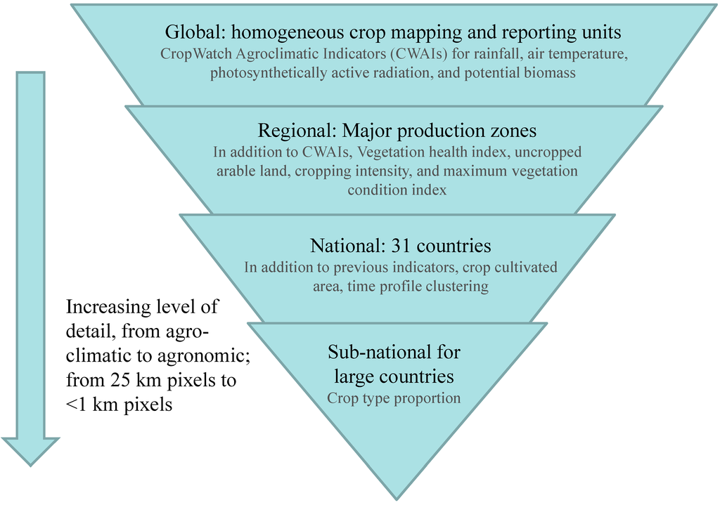
Figure 1.
CropWatch hierarchical crop monitoring approach.
2.1. Spatial Scale
2.1.1. Global Crop Monitoring and Reporting Units (MRU)
Sixty-five MRUs are used at the highest (global) level, mostly for environmental indicators. The main basis for the delineation of the MRUs is the global ecological map prepared in the ambit of the FAO Forest Resources Assessment [34], further subdivided when necessary or otherwise modified based mainly on Köppen climate zones [35,36] and the “most suitable cereal” grids available from the Global Agro-Ecological Zones (GAEZ) project [37]. Other sources include the major crop area and climate division from USDA [38], global distribution of cultivable lands from Ramankutty, et al. (2002) [39] and the crop area from Monfreda, et al. (2008) [40]. Figure 2 locates the sixty-five zones [41]. For China, the agricultural zones from Sun (1994) [42] are adopted, which divide the country into 9 geographic regions (Figure 3) of which only seven are relevant for production estimates.
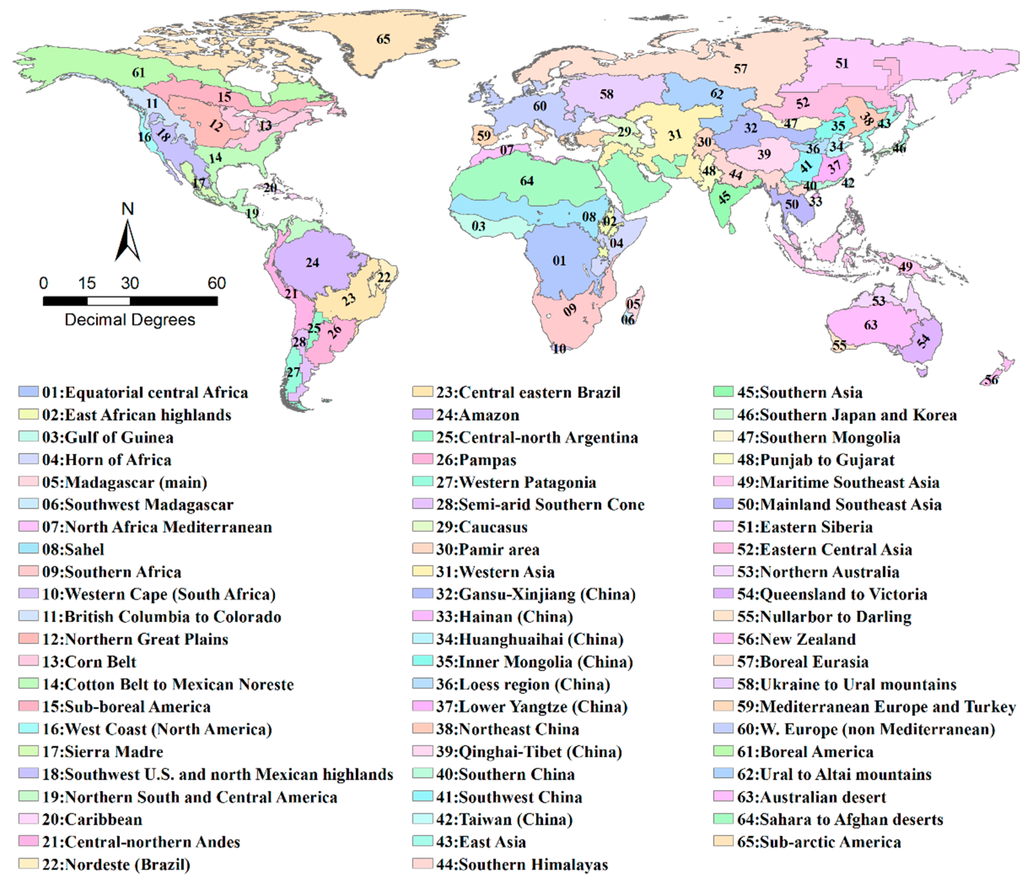
Figure 2.
Sixty-five Monitoring and Reporting Units of the CropWatch system.
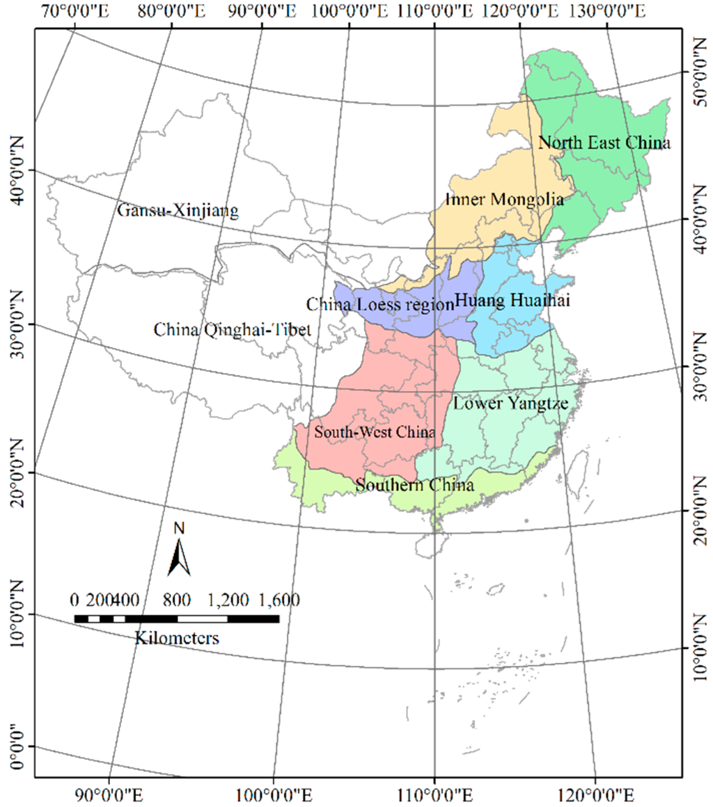
Figure 3.
Seven crop monitoring sub-divisions adopted by the CropWatch System for China (modified from Sun (1994) [42]).
2.1.2. Major Production Zones (MPZs)
The MPZs are used for regional analyses. The zones were selected based essentially on global digital crop maps developed by Monfreda et al. (2008) [40]. The seven MPZs currently selected include West Africa (maize), North America (wheat, maize and soybean), South America (maize, soybean), South and Southeast Asia (rice), Central Europe and Western Russia (barley, wheat and potato), Western Europe (wheat, maize, barley and potato) and Southern Australia (wheat) with at least one major crop cultivated in each MPZ. Figure 4 illustrates the seven MPZs. In the future, white potato and barley (major contributors to food security worldwide) will be included in the CropWatch crop monitoring list.
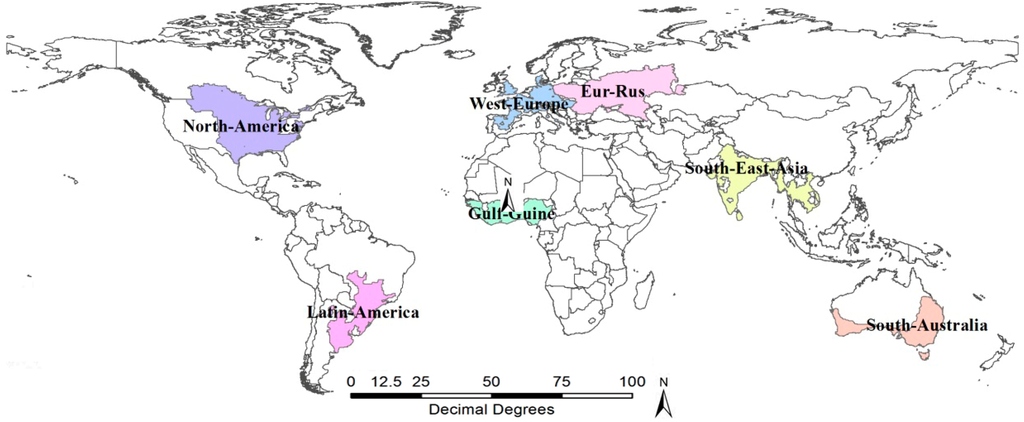
Figure 4.
Major Production Zones in the CropWatch system.
2.1.3. Countries and Sub-Country Units
The thirty-one key countries selected by CropWatch for global agricultural monitoring represent more than 80 percent of global production and exports of maize, rice, wheat and soybean according to FAO statistics [43]. Some countries were selected not specifically for their contribution to food production, but because of their relevance as Asian neighbors of China and their importance for food security, as illustrated by the inclusion of four out of the five most populated countries in Africa. Figure 5 shows the distribution of thirty-one countries. For some of the larger countries (Argentina, Australia, Brazil, Canada, China, India, Kazakhstan, Russia, and the United States), main administrative subdivisions are included in the analyses.
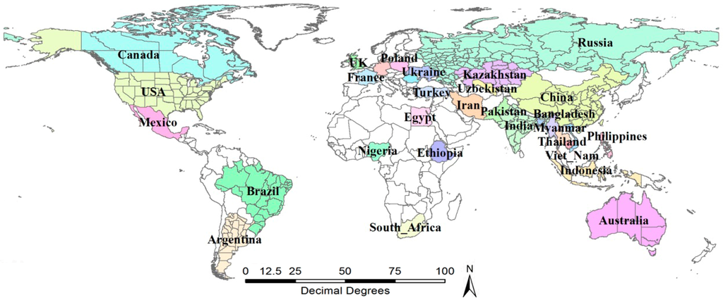
Figure 5.
Thirty-one key countries in the CropWatch system.
2.2. Indicators
Table 1 illustrates different indicators for different scales in CropWatch. They can be divided into four categories: CropWatch agroclimatic indicators (CWAIs), arable land use intensity indicators, crop condition indicators and crop production indicators. Some indicators are used at multiple scales, but with different resolution. For each scale of analysis, outputs from larger scales are also considered with additional outputs at current scale. For instance, rainfall (R), air temperature (T), photosynthetically active radiation (PAR) and potential biomass (BIO) are computed at the global scale to capture global abnormal weather patterns but also at all intermediate scales down to sub-national. At sub country scale, all the indicators listed in Table 1 are used as inputs. All the information including abnormal weather patterns, unusual cropping patterns, crop condition and production as well as crops opted for by farmers will be generated at sub-national scale as outputs.

Table 1.
Hierarchical indicators of CropWatch. For each scale of analysis, all the indicators of the row above are also produced. (R = CWAI for rainfall; T = CWAI for air temperature; PAR = CWAI for photosynthetically active radiation; BIO = agroclimatic biomass production potential; CI = Cropping intensity; CALF = Cropped arable land fraction; VHI = Vegetation health index; VCIx = Maximum vegetation condition index; CTP = Crop type proportion).
| Scale | R | T | PAR | BIO | CI | CALF | VHI | VCIx | NDVI | CTP | Outputs |
|---|---|---|---|---|---|---|---|---|---|---|---|
| Global | + | + | + | + | Abnormal weather pattern | ||||||
| MPZs | + | + | + | + | + | + | + | + | Unusual cropping pattern | ||
| 30+1 key countries | + | + | + | + | + | + | + | + | + | Crop condition and production | |
| Sub countries | + | + | + | + | + | + | + | + | + | + | Crops opted for by farmers |
2.2.1. Agroclimatic Indicators
The CropWatch Agroclimatic Indicators (CWAIs) describe environmental crop growing conditions and their departure from “normal” for R, T, PAR and BIO. The four indicators are calculated based on global grids of rainfall, air temperature, PAR and potential biomass with spatial resolution of 25 km. The rainfall product is generated based on TRMM data sets [44], ERA-Interim (ERA-I) and ECMWF Operational (ERA OPE) dekad rainfall products [45]. The global air temperature is interpolated from over 9000 station measurements from the Global Surface Summary of the Day (GlobalSOD) [46] with ordinary Kriging. Potential biomass is adapted from the Miami Model [47] to express the maximum possible net primary production (NPP) for a certain area assuming rainfall and temperature are the only constraints. NPP is calculated using temperature and rainfall, and the minimum value is used as the potential biomass in CropWatch. For a given polygon and time interval, each CWAI is computed only over agricultural areas and using long-term average potential biomass as weighting factor (the higher potential biomass the pixel presents, the more weight it is given) [48,49]. The potential biomass departure is computed as the difference between accumulated biomass of the current season and the average of recent five years.
2.2.2. Arable Land Use Intensity Indicators
In addition to agro-climatic indicators, CropWatch analyses also resort to other indicators to assess the condition of the crops for major production zones and thirty-one key countries. The indicators fall into two categories: arable land use intensity and crop condition.
Indicators for arable land use intensity include cropping intensity (CI) and cropped arable land fraction (CALF). The CI describes the extent to which arable is used over a growing season. It is the ratio of total crop area of all planting seasons in a year to the total area of arable land [50]. CropWatch adopts the method proposed by Fan and Wu (2004) [50] based on an NDVI time-series derived from MODIS Terra and reconstructed by the Savitzky and Golay (S-G) filter [51]. CALF is introduced to express the proportion of currently cropped arable land in the total arable land over countries and sub-national units over a certain period (monthly, seasonally, or annually). CALF is based on a NDVI threshold method combined with a decision tree to identify whether an agricultural pixel is cropped or uncropped. Monthly CALF can reveal the dynamic change of cropped arable land area [52].
2.2.3. Crop Condition Indicators
Crop condition indicators include the Vegetation Health Index (VHI) [33], maximum Vegetation Condition Index (VCIx), crop condition development assessed by NDVI, and spatial clustering of NDVI departure from average and the corresponding cluster profiles. VCIx indicates the relative value of the current crop condition over the monitoring time window compared with historical data. Values for VCIx usually vary from 0 to 1, where the high values are better crop condition and low values indicate worse crop condition. VHI is an effective indication of the crop stress which is calculated by averaging the VCI [53] and Temperature Condition Index (TCI). VHI is a combined indicator to monitor effect of both rainfall and temperature on crops [54].
For crop condition monitoring, an NDVI-based method is employed to evaluate crop condition by inter-annual comparisons of both spatial variability (using NDVI images) and seasonal dynamics (based on NDVI profiles [55,56,57]).
Based on a time series of pixel-based (raster) images, time profile clustering is a method that compares the time profiles of all pixels and distributes them among a limited number of “typical” behaviors (classes) that can be mapped [58,59,60]. Profiles of NDVI and VHI departure from the average of the last five or twelve years are clustered in CropWatch for MPZs, countries and subdivisions of large countries. The clustering method has the advantage of synthetically describing the characteristics of spatial distribution of typical time profiles.
2.2.4. Crop Production Indicators
CropWatch adopts different crop area estimation methods for different countries. For China, remotely sensed estimates of arable land area and CALF are combined with field survey based estimates of crop type proportion (specific type area to total cropped area, also referred to as “cropping structure”) [61,62]. For other thirty key countries and provinces/states of eight large countries (the United States, Russia, India, Argentina, Brazil, Australia, Canada and Kazakhstan), CALF is used to estimate individual crop area using the following equation:
where i is the current year; a and b are linear regression coefficients between cropped area from FAOSTAT [43] or, preferably, sub-national data when available at the website of Ministry of Agriculture or National Bureau of Statistics. If no significant regression is found, crop area is assessed based on other sources, including international and national forecasts and reports.
As for yields, due to the differences in data availability, contrasting approaches are applied for China and for other thirty countries. For China, three models, namely an agro-meteorological model, a remote sensing index model and biomass-harvest index model are applied based on agro-climatic indicators, crop condition indicators and station-based agro-meteorological observations [3,63,64,65,66], calibrated with more than 600 agro-meteorological station data. The yields pooled from different models are combined and averaged to predict the crop yield per spatial unit.
For other thirty key countries and sub-national administrative units, the average phenology from easily available sources such as USDA [67] and FAO/GIEWS [68] is used to determine the growing season. Average and maximum NDVI of the growing season for current year and reference year over a crop specific mask combined with the yield of the reference year are used to calculate the yield of the current year for the four crops (maize, wheat, soybean and rice) using the following equation:
where i is the current year and r is reference year; yield of the reference year is from FAOSTAT or from national sources when available. NDVIi and NDVIr refer to the NDVI profile of the current season and the reference season, respectively. Max (NDVI) and mean (NDVI) are the maximum NDVI and average NDVI of the whole growing season. Abundant literature confirms that maximum NDVI or average NDVI during the growing season is strongly related with crop yield [69,70,71,72], etc. The selection of either max (NDVIi)/max (NDVIr) or mean (NDVIi)/mean (NDVIr) is based on the impact of clouds on the NDVI signal. If peak NDVI is severely impacted by clouds, mean (NDVIi)/mean (NDVIr) is be used to represent yield variation. Otherwise, max (NDVIi)/max (NDVIr) is preferred. In deciding whether max(NDVIi)/max(NDVIr) or mean(NDVIi)/mean(NDVIr) is used in Equation (2) for different countries and regions we follow the approach outlined by Huang et al. (2013) [72] in their overview of NDVI-based yield forecasting approaches for maize, rice, wheat and soybean.
For each crop type, yield is forecast before harvesting and subsequently revised after harvest using the above method. Forecasts use actual data up to the time of the forecast and “average” data between the time of the forecast and harvest; post-harvest estimates use only actual current season data.
2.3. Crop Supply Situation Outlook Analysis
The CropWatch global crop supply outlook includes long-term trends and short-term dynamic changes, and follows a methodology based on three-year simple moving average (SMA) that has been in use for the last 15 years:
where SMA (j, i) is the value computed for year i and crop j based on the production of the three previous years. SMA (j, i +1), the projected value for the next years is given by Equation (4). The comparison of SMA (j, i+1) with SMA (j, i) indicates whether the short-term supply prospects are improving or deteriorating.
3. Typical Outputs
3.1. Analysis of Indicators
3.1.1. Global Agroclimatic Assessment at the Global Scale
The CropWatch agroclimatic indicators (CWAIs) identify the global patterns of extreme factors which might affect agricultural production and assess the impact of climate at the global scale. Figure 6, Figure 7 and Figure 8 illustrate three indicators (temperature, rainfall and potential biomass) at different spatial scales.
Figure 6 shows a cold spell that affected vast expanses of land in Eurasia, including northwest India, parts of China, central Asia and Europe, and North America in the first quarter of 2013 (January to April 2013). Figure 7 presents the dry conditions that affected large areas of the southern and northern Mediterranean, as well as adjacent countries in central Europe from October 2013 to January 2014. Figure 8 shows the poor biomass accumulation during January to April 2014 that prevailed in eastern-central Asia, northeast China, southern China, East Asia, two Mediterranean MRUs (northern Africa and Mediterranean Europe, and Turkey), as well as North America, large areas of Mexico and central America and northeast Brazil. In contrast, some large and very large positive biomass departures are identified in Asia (Gansu-Xinjiang; Mongolia region; Punjab to Gujarat), in Africa (Sahel; Western Cape area in South Africa,), and in South America (some of the major agricultural areas in Brazil and Argentina).
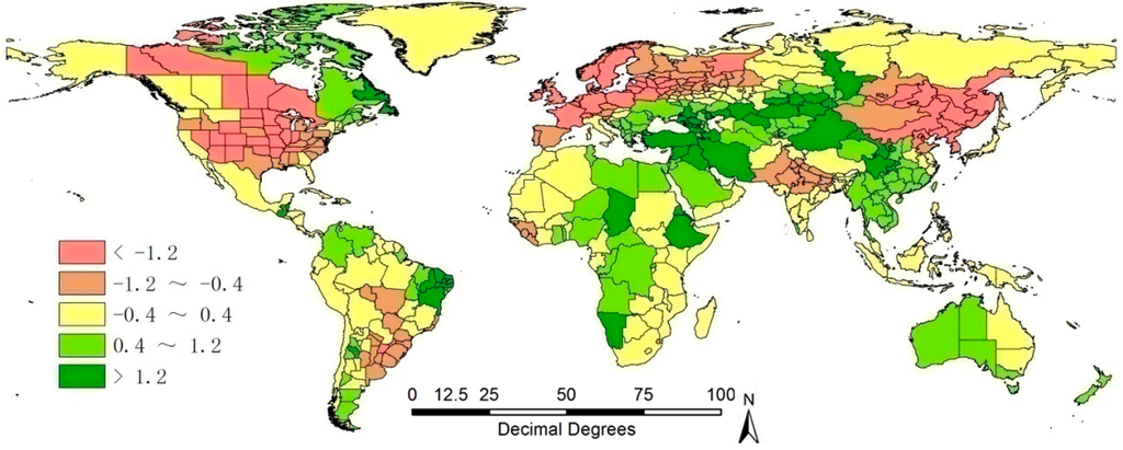
Figure 6.
January to April 2013 global map of temperature departure from the 2002–2012 average, by country and administrative subdivisions within large countries; the difference is expressed as degrees Celsius (°C).
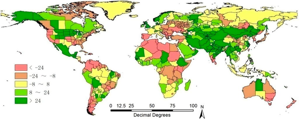
Figure 7.
October 2013 to January 2014 global rainfall departure from the 2001–2012 average, by country and large administrative areas within large countries; the difference is expressed as percentage of the reference (%).
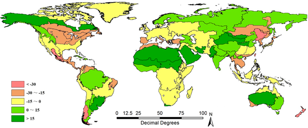
Figure 8.
January to April 2014 global map of potential biomass departure from the 2001–2013 average, over sixty-five crop Mapping and Reporting Units; the difference is expressed as percentage of the reference (%).
3.1.2. Arable Land Use Intensity Monitoring at MPZ Scale
The CI and CALF are used by CropWatch to assess the arable land use intensity. Figure 9 and Figure 10 show the CI map in 2013 and the cropped and uncropped arable land maps of different time periods from January 2013 to January 2014 for Western Europe. CI for Western Europe was 132% in 2013, five percent above the previous five-year-average. Most of farmlands with double cropping system are located in France, Germany, the United Kingdom (UK), Czechoslovakia, and Denmark while single cropping system dominates Spain. Figure 10 indicates that much arable land is under-cropped in 2013 except for the regions in Central Spain. Land use differences between January and April 2013 and October 2013 and January 2014 occur mainly in two areas: central Spain, and south-eastern France and north-west Italy. In general, 96% of arable land was cropped from January to December 2013, 2% higher than the previous five years average.
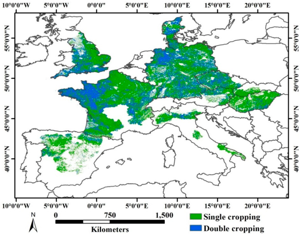
Figure 9.
Cropping intensity map for Western Europe in 2013.
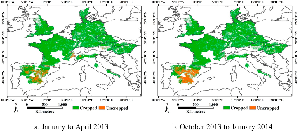
Figure 10.
Cropped and uncropped arable land map for Western Europe over two time intervals. (a) January to April 2013; (b) October 2013 to January 2014.
3.1.3. Crop Condition at Country Scale
VCIx, the graph of crop condition development based on NDVI, clusters of the time-series NDVI departure and the vegetation health index (VHI) departure are adopted for crop condition assessment. The indicators reflect different facets of crop condition in the main production zones and countries. VCIx between January and July 2014 (Figure 11) indicated that crop condition was generally above average in the main corn, soybean and cotton belt in the Contiguous United States (CONUS). Crop condition was below average resulting from a significant decrease of rainfall between January and April 2014 in Texas (−53%), Oklahoma (−47%), Kansas (−44%) and Nebraska (−23%). Other States suffered from water shortage between April and July 2014 including: California (−33%), Oregon (−41%), Washington (−28%), and Idaho (−21%). Reports from USDA, National Agricultural Statistics Service (NASS) [73] confirm CropWatch analyses.
Variations of crop condition are described based on NDVI development in Figure 12. Crop condition was below the historical average before mid-June due to the double impact from drought and abnormally low temperature. After mid-June, while winter wheat harvest was ongoing, maize, soybean and rice benefited from abundant precipitation and suitable temperature. Crop condition recovered to reach the previous five-year average.
Spatial variations over different regions are presented by clusters of NDVI departures in Figure 13 between January and July 2014. In the main soybean and maize belt (Minnesota, Iowa, Wisconsin, Michigan, Indiana), NDVI departure from average profiles indicate poor crop condition during January and June due to significant decrease of PAR and abnormally low temperature. In the main winter wheat zone, the crop condition was below average, due to serious drought in Texas and Oklahoma. In the main rice zone, the crop condition was persistently above average thanks to favorable weather.
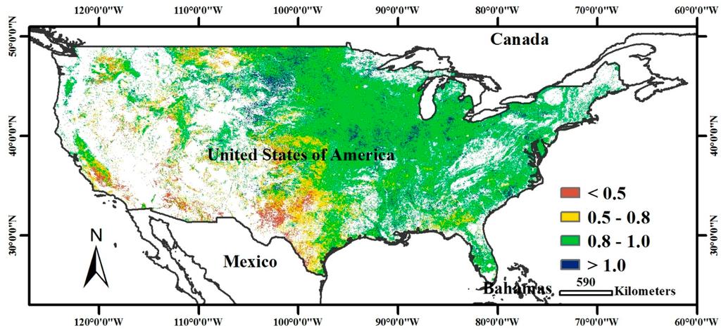
Figure 11.
Spatial distribution of the VCIx between January and July 2014 in the CONUS.
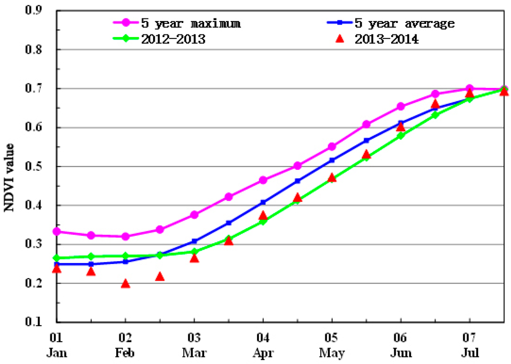
Figure 12.
Comparison of various NDVI profiles over the maize, wheat, rice and soybean mask for CONUS.
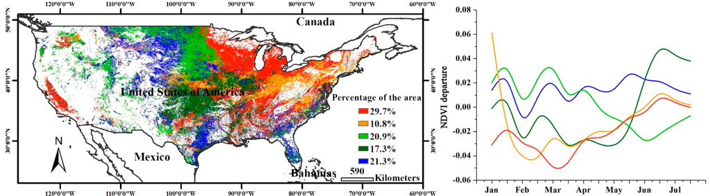
Figure 13.
(a) The Spatial distribution of NDVI departure cluster during January and July 2014 in the United States; (b) The NDVI departure profiles associated with (a). The horizontal line marks “0 departure”, i.e., average conditions.
As a key descriptor of crop condition, the VHI departure cluster in Figure 14 indicates the water and temperature stress at different growing stages. In the period from January to July of 2014, crop condition in California and the south Texas was persistently below average due to serious water stress. In the western parts of the soybean and corn belt, VHI was below average after April due to excessive rainfall and abnormally low temperature from January to April in Iowa (+58%), South Dakota (+37%) and Minnesota (+33%). VHI departure indicates that Washington, Oregon, some parts of Texas, Oklahoma, and Kansas suffered from serious water stress, as also described in the section on VCIx. The positive VHI departure in other regions indicates adequate water supply and favorable temperature.
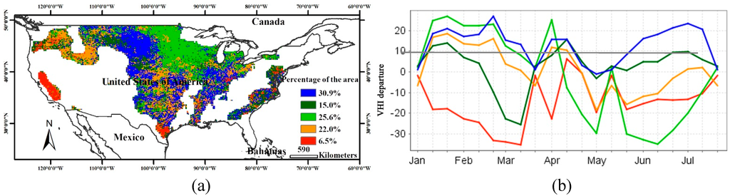
Figure 14.
(a) The Spatial distribution of VHI departure cluster in the United States; (b) The VHI departure profiles associated with (a); the horizontal line denotes average conditions.
3.1.4. Crop Type Proportion for Provinces in China
Crop type proportion for China, i.e., the distribution of arable land between different crop types, is shown in Table 2 for four major crops only. The table immediately shows the relative importance of summer crops in terms of cultivated land: maize: 52 percent; rice: 19 percent; soybeans: 6 percent. The provinces where maize occupied more than 70 percent of summer cultivated land include Guizhou, Hebei, Henan, Inner Mongolia, Jilin, Liaoning, Ningxia, Shaanxi, and Shanxi, while Guangxi, Hunan, and Jiangsu cultivates very little. It is a characteristic of the maize proportion in Table 2 that the crop either plays a dominant part, or almost no part. There are no “intermediate” provinces. For rice, the focus (>40 percent of land) is in Guangxi, Hunan, Jiangsu, and Sichuan; and many provinces do not cultivate rice at all. As for soybean, it remains a subordinate crop, except for Anhui (30 percent) and the three provinces of Guizhou, Heilongjiang and Henan where it occupies between 10 and 15 percent of the land. Henan and Shandong are the provinces which, by far, cultivate the largest proportion of wheat. Spring wheat is insignificant except for Gansu, Heilongjiang, Inner Mongolia and Ningxia. The bulk of the production, however, originates in Henan, Shandong, Hebei, Jiangsu, and Anhui.
Table 2.
Crop type proportion for China 2013. Note: The numbers indicate the percentage of the area cultivated under maize, rice, and soybean during early July and early October, and under wheat during mid-May in 2014. The difference between 100 percent and the sum of maize, rice, and soybean per province is “other summer crops”. * Fujian, Guangdong, Jiangxi, and Zhejiang were not sampled because rice is by far the dominant crop among the four major crops.
| City | Maize | Rice | Soybean | Wheat |
|---|---|---|---|---|
| Anhui | 28.86 | 26.76 | 24.17 | 39.21 |
| Chongqing | 52.69 | 26.49 | 3.46 | 19.83 |
| Fujian * | ||||
| Gansu | 50.57 | 0.09 | 0.49 | 25.27 |
| Guangdong * | ||||
| Guangxi | 6.29 | 45.88 | 0.08 | |
| Guizhou | 82.12 | 2.36 | 15.49 | |
| Hebei | 76.58 | 0.02 | 0.34 | 36.79 |
| Heilongjiang | 60.68 | 21.69 | 15.03 | 1.32 |
| Henan | 74.27 | 0.01 | 11.42 | 68.80 |
| Hubei | 21.81 | 38.31 | 1.03 | 16.36 |
| Hunan | 9.37 | 71.61 | 0.29 | |
| Inner Mongolia | 77.49 | 0.05 | 0.29 | 5.10 |
| Jiangsu | 3.87 | 50.70 | 5.94 | 40.71 |
| Jiangxi * | ||||
| Jilin | 79.09 | 14.03 | 1.65 | |
| Liaoning | 80.85 | 7.56 | 0.42 | |
| Ningxia | 72.30 | 13.98 | 0.00 | 20.03 |
| Shaanxi | 71.54 | 7.65 | 0.37 | 18.57 |
| Shandong | 54.58 | 0.00 | 0.18 | 57.80 |
| Shanxi | 75.50 | 0.00 | 1.08 | 15.74 |
| Sichuan | 28.89 | 44.68 | 3.63 | 28.46 |
| Yunnan | 47.22 | 12.78 | 1.97 | |
| Zhejiang * | ||||
| China | 52 | 19 | 6 |
3.2. Food Supply Situation
3.2.1. Global Crop Supply Prospects
Based on the three year moving average approach, CropWatch prepared the production outlook for 2013 shown in Figure 15.
The current general and global dominance of maize continues, followed by rice and wheat. In the recent five years, the global rice and soybean production presented a steady increase. Although the global production of wheat and maize both show a decreasing trend in the recent four years, the production of both increased spectacularly in 2013. According to the monitoring result in January 2014, a positive trend was observed for wheat production in the southern hemisphere, resulting in improved supply prospects.
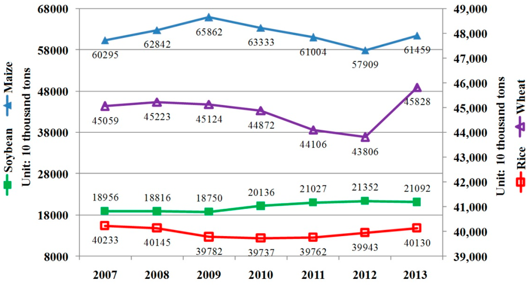
Figure 15.
Three year moving average production of maize, rice, wheat and soybean of major producers.
3.2.2. Production Estimates
The latest CropWatch production estimate for the 2014 season puts the production of maize and rice (as paddy) at 993,783 and 755,513 thousand tons, respectively, both at about the same level as 2013; wheat is up 2% (compared to last year) with 719,718 thousand tons, while soybean reaches 294,822 thousand ton, a significant increase (+6%) over the previous harvest (Table 3).
When only major producers are considered, the situation is slightly less favorable for maize (−1% compared to last year), similar for rice (0%) and wheat (+2%), but significantly better for soybean (+9%), indicating that minor soybean producers keep losing ground compared with the big three: United States, Brazil, and Argentina. The figures also confirm that maize and rice continue consolidating their global dominant role in cereal production (mostly at the expense of spring wheat).
For the major exporters, production has basically stagnated, except for soybean for which their offer may increase.
Table 3.
Global 2014 production of maize, rice, wheat, and soybean (thousand tons) and departure from 2013 production (estimates issued in the November 2014 CropWatch bulletin).
| Maize | Rice | Wheat | Soybean | ||
|---|---|---|---|---|---|
| Total production | 993,783 | 755,513 | 719,718 | 294,822 | |
| Departure from 2013 production (%) | World | 0 | 0 | +2 | +6 |
| Top 80% producers | −1 | 0 | +2 | +9 | |
| Rest of the world | +9 | +6 | −23 | −26 | |
| Major exporters | −1 | 0 | 0 | +7 |
Note: Departures expressed as percentage compared to 2013 production.
4. Discussion
This paper proposes a hierarchical method for global crop monitoring. A four tier monitoring strategy was developed: global (sixty-five MRUs), regional (seven MPZs), national (thirty-one key countries) and sub-national (subdivisions of nine large countries). Thirteen climatic and remote sensing monitoring indicators have been selected for different scales to best characterize the agricultural information at the corresponding scale. The thirteen indicators can be regrouped into two categories: CWAIs and crop or “agronomic” indicators. The former describes the influence of weather factors while the latter describe crop condition and development. The global rain, temperature, PAR and potential biomass products are used to estimate the influence of climate factors and to analyze crop growth from the agroclimatic perspective.
Production estimation is a major output, but not the only one: Thirteen indicators provide much information at different scales and some of them (CWAIs and CALF) can provide early warning information.
The new method discards the classical country-based approach to global monitoring and adopts different scales for different indicators. “Global”, i.e., planetary crop monitoring is usually understood as the monitoring of all countries worldwide in a piecewise and rather static way.
Starting at the highest level, CWAIs are used to look at agro-climatic patterns globally computed based on rainfall, temperature and PAR at a spatial resolution of 25 km. They are spatial averages over the polygons, but limited to cropped areas and weighted so that higher importance is given to areas with high production potential. Although they are expressed in the same units as the underlying climatic variables, the CWAIs are highly value-added indicators. They are first computed for sixty-five MRUs that cover the whole globe. The MRUs correspond to very broad crop production areas. Significantly more units would be required to capture crop geography realistically, but the purpose is to identify global environmental patterns that, experience shows, often affect whole continents. For instance, CropWatch identified the cold spell that occurred over much of the northern hemisphere in early 2013, or the circum-Mediterranean drought that affected late 2013 and early 2014.
MRUs are actually based on large agro-ecological zones, but the rather “broad” terminology of MRU was adopted for the highest level because the CWAIs can actually be used over different polygons at any scale (because their computation covers only agricultural areas). It remains that CWAIs provide little information about when exactly abnormal conditions occurred.
The scale below MRUs is that of seven MPZs, where, next to CWAIs the new system adds (1) time profiles and (2) agronomically meaningful indicators, especially the area of cropped arable land as CALF. CALF provides early warning information on crop production. VCIx assesses the current crop status compared with the situation during the last 5 years, which gives a hint of what the crop yield level will be; next, VHI gives additional explanation if water stress is the reason.
Abnormal conditions are measured by the departure of the indicators from the historical average (currently 2001 to 2013), a period that is sufficiently long to have some climatological significance, but sufficiently short to remain agronomically meaningful. Future analyses will gradually adopt fourteen and eventually fifteen years reference periods and then stay at fifteen.
Once general patterns have been identified and described, additional tools must be brought in to look into crop condition. For the agronomic indicators, to take into account the short-term adaptability of farming, the reference period of five years was adopted.
Crop or “agronomic” indicators such as CI, CALF, VCIx, VHI and NDVI profiles allow the analyst to infer crop condition and development. The new CropWatch system takes full advantages of multiple sources of remotely sensed data and delivers more information than the traditional approach which is based on area and yield to get the production. The indicators are most useful for decision makers: The CI effectively measures changes in arable land use intensity (number of crops per year in a given area). VCIx compares the current crops against historical data from the last five years. All the mentioned crop indicators can provide early assessments of crop productions, which provide decision makers with separate and independent measures about future crop prospects.
The same indicators as above are resorted to at the national scale and for Chinese regions, adding more details about the development of the season by looking at average NDVI as well as spatial differences in NDVI profile patterns.
The global crop supply prospects have shown their usefulness. In the long run, it is certainly desirable to develop global crop intelligence systems that have predictive capacity for a broader spectrum of variables, and that are relevant for trade and food security planning, covering the current season and possibly further ahead by incorporating seasonal (climate) forecasts.
Multiple domestic and international remote sensing data sources have been adopted in CropWatch, including TRMM, FY-3A, MODIS, HJ-1, GF-1, ZY-3 and Landsat 8 satellite images. Over sixteen years of continuous operation, CropWatch assembled historical data of area, yield and production covering thirty-one countries in addition to ground measurements and inventories. Of special mention are the collection of the crop type proportion, in situ biomass and yield, and production data of the main producing provinces in China. The new remotely sensed data used in CropWatch reduce the dependence on traditional field observations.
The validation and the accuracy assessment of CropWatch indicators are beyond the scope of this paper. As a matter of fact, the accuracy of the used remote sensing product relies on other studies that assessed, directly and indirectly, the accuracy of the product. In our particular case we rely on the studies of TRMM product validation [74,75,76], air temperature and PAR validation [48], and the applications of VCI, TCI and VHI [33,54,77,78]. In particular, CALF, crop type proportion and crop area have been validated intensively over last 10 years [3,52,62]. The same products used in this paper were used with success in other studies [2,19,20].
A rigorous “running” validation process is adopted and ensures the stable operation of the CropWatch system and at the same time feeds its progress, making it a cutting edge agricultural monitoring system. Starting in 2012, more than eight hundred samples covering planting area and production of maize from close to three hundred sample plots were collected to monitor and validate the crop production at the provincial scale in China. Data from 600 agro-meteorological sites over China are used to calibrate the yield model. The field work for validating CropWatch indicators takes place at twenty-eight global sites [1,52,55,,56,61,62,63,79,80,81,82,83,84,85,86,87,88,89,90,91,92,93,94,95].
The purpose of the international analyses also includes the development of new indicators and an upgraded operational methodology. Although the current focus is on food security and market planning for major commercial crops, the methods developed have potential as well for other applications in rangeland monitoring, risk assessment and crop insurance, to name just a few.
The thirteen indicators describe spatial patterns well. There are, however, some weaknesses that need to be mentioned: the impact of unequal distribution of rainfall, cold spells or reduced sunshine are insufficiently taken into account. Additional indicators are needed to better assess soil moisture and the effect of transient adverse factors on crops, including some that are currently not systematically included (such as potatoes or barley). Research is needed as well to model impacts of extreme factors, i.e., those that physically damage crops (such as frost, or extreme wind speeds associated with tropical cyclones). These factors cannot currently be modeled with sufficient accuracy, which is why they are not integrated with other indicators by the existing crop monitoring systems.
Another weakness is indeed the fact that CropWatch is still very indicator-oriented. It is, somehow, paradoxical that the sophisticated models are basically unsuited for routine crop monitoring, because the scale of crop monitoring (mostly administrative areas) has to be compatible with the scale of socio-economic variables, such as population and food requirements. Most inputs of process-oriented models are not compatible with that scale, and many crop model parameters (such as soil moisture holding capacity, or crop ecophysiology, including phenology, cycle length) are just meaningless at the regional scale. The result is that simple models, even semi-impressionistic ones (descriptive or non-parametric) are strongly needed to be applied in regional crop monitoring.
By definition, crop monitoring is a very dynamic activity which requires that research on algorithms and methods on crop condition assessments and forecasts be continuously monitored. This is one of the reasons why post-factum evaluation of the past performance of forecasts is, somehow, pointless; it would be meaningful only if the same method/data had been used for several years. In practice, methods change over time and so do available data sources, almost annually. As a result, forecasts/estimates produced during earlier years are no longer comparable with those obtained with current methods. Even within the same season, early estimates include both historical data (up to the time of forecast) and “future data” (usually assumed to be “average”, although other approaches are possible). Actually, the continuous calibration and re-calibration of the forecasting method with the “best” current data and methods actually plays the part of the post-factum evaluation of model performance.
In 2014, CropWatch proposed a new method to retrieve adjusted NDVI for cropped arable land during the growing season by integrating time-series MODIS NDVI images and cropped and uncropped arable land use maps [96]. Based on the adjusted NDVI, more accurate crop condition monitoring results are achieved simply by removing the variance in NDVI that is caused by the change in crop area, not the crop condition [96]. The new proposed method for crop condition monitoring is still at development stage. All potential new analytical methods for CropWatch undergo extensive validation throughout the globe before being incorporated into the operational system.
5. Conclusions
A new satellite-based hierarchical method of global crop monitoring is adopted by CropWatch. The new approach reports crop impacting factors (mostly agro-climatic) over sixty-five MRUs with 4 indicators and cropping intensity at global scale and stress (satellite-based) over 7 MPZs with 4 additional indicators. Five additional indicators allow the analyst to infer crop condition and development at national and sub-national scale. Global crop monitoring is no longer a simple combination of national crop monitoring methods. Thanks to the use of nested indicators of increasing spatial and temporal resolution from the global scale to the national and sub-national scale, an integrated assessment is developed in which “the tree does not hide the forest”. Global and continental patterns are identified before zooming into regions, countries and sub-national units, which can thus be described in a more synthetic fashion.
With thirteen hierarchical indicators, production estimation remains an essential but no longer the main output. The thirteen indicators provide more outputs at different scales than national production, for instance early warning messages for the global grain market, especially the CALF indicator and the analyses for the seven MPZs.
The hierarchical analyses of climatic and crop conditions assessments are published in the quarterly “CropWatch bulletin” [97], which also provides a detailed overview of data and methods.
Acknowledgments
This paper was funded by National High Technology Research and Development Program of China (863 program) (Grant No. 2012AA12A307 and 2013AA12A302), the Program of International Science and Technology Cooperation (Grant No. 2011DFG72280) and Special Fund for Grains-scientific Research in the Public Interest (Grant No. 201313009-2 and 201413003-7).
Author Contributions
Bingfang Wu, the corresponding author and leader of the CropWatch group, developed the concept and architecture of the CropWatch system; he contributed to the overall approach, introduction and discussion sections of this manuscript. René Gommes proposed the hierarchical crop monitoring approach for CropWatch, designed the MRUs and MPZs as the basic analytical units, and contributed to the sections on the global agroclimatic assessment, food supply situation, and production estimates. Miao Zhang is responsible for both method and results of the arable land use intensity indicators and also contributed to the discussion section. Hongwei Zeng, Nana Yan, Wentao Zou, Yang Zheng and Ning Zhang are the developers of one or several indicators and the writers of the corresponding results sections in the manuscript. Sheng Chang and Qiang Xing described the results for the major production zones and crop condition at country level. Anna van Heijden provided many suggestions during manuscript preparation and helped review the text. Data processing and results analysis were done by all the listed authors.
Conflicts of Interest
The authors declare no conflict of interest.
References
- Wu, B.; Meng, J.; Li, Q.; Zhang, F.; Du, X.; Yan, N. Latest development of “CropWatch”—An global crop monitoringsystem with remote sensing. Adv. Earth Sci. 2010, 25, 1013–1022. [Google Scholar]
- Becker-Reshef, I.; Justice, C.; Sullivan, M.; Vermote, E.; Tucker, C.; Anyamba, A.; Small, J.; Pak, E.; Masuoka, E.; Schmaltz, J.; et al. Monitoring global croplands with coarse resolution earth observations: The global agriculture monitoring (GLAM) project. Remote Sens. 2010, 2, 1589–1609. [Google Scholar] [CrossRef]
- Wu, B.; Meng, J.; Li, Q.; Yan, N.; Du, X.; Zhang, M. Remote sensing-based global crop monitoring: Experiences with China’s CropWatch system. Int. J. Dig.Earth 2014, 7, 113–137. [Google Scholar] [CrossRef]
- MinAgri—Argentina. Available online: http://www.minagri.gob.ar/site/ (accessed on 31 May 2014).
- Fontana, D.C.; Melo, R.W.; Wagner, A.P.L.; Weber, E.; Gusso, A. Use of remote sensing for crop yield and area estimates in the southern of Brazil. Int. Arch. Photogramm. Remote Sens. Spat. Inf. Sci. 2006, 36, 8/W48. 53–58. [Google Scholar]
- Reichert, G.C.; Caissy, D. A Reliable Crop Condition Assessment Program (CCAP) Incorporating NOAA AVHRR Data, a Geographical Information System and the Internet. Available online: http://proceedings.esri.com/library/userconf/proc02/pap0111/p0111.htm (accessed on 22 March 2013).
- Space Applications Centre (SAC). Manual for Crop Production Forecasting Using Remotely Sensed Data, a Joint Project of Space and Ministry of Agriculture; Space Applications Centre: Ahmedabad, India, 1995.
- Sivakumar, M.V.K.; Gommes, R.; Baier, W. Agrometeorology and sustainable agriculture. Agric. For. Meteorol. 2000, 103, 11–26. [Google Scholar] [CrossRef]
- Gommes, R. Agrometeorological models and remote sensing for crop monitoring and forecasting. In Proceedings of the Report of the Asia-Pacific Conference on Early Warning, Preparedness, Prevention and Management of Disasters, Chiang-Mai, Thailand, 12–15 June 2001.
- Adams, R.M.; Houston, L.L.; McCarl, B.A.; Tiscareño, M.L.; Jaime Matus, L.; Weiher, R.F. The benefits to Mexican agriculture of an El Niño-southern oscillation (ENSO) early warning system. Agric. For. Meteorol. 2003, 115, 183–194. [Google Scholar] [CrossRef]
- Balaghi, R.; Badjeck, M-C; Bakari, D.; de Pauw, E.; de Wit, A.; Defourny, P.; Donato, S.; Gommes, R.; Jlibene, M.; Ravelo, A.C.; et al. Managing climatic risks for enhanced food security: Key information capabilities. Procedia Environ. Sci. 2010, 1, 313–323. [Google Scholar] [CrossRef]
- Begum, S.; Nessa, M.; Alam, M.S. Space technology for crop monitoring of Bangladesh. Res. J. Sci. IT Manag. 2013, 2, 11–17. [Google Scholar]
- Fakhruddin, S.H.M.; Chivakidakarn, Y. A case study for early warning and disaster management in Thailand. Int. J. Disaster Risk Reduct. 2014, 9, 159–180. [Google Scholar] [CrossRef]
- Pulwarthy, R.S.; Sivakumar, M.V.K. Information systems in a changing climate: Early warnings and drought risk management. Weather Clim. Extremes 2014, 3, 14–21. [Google Scholar] [CrossRef]
- Mock, N.; Morrow, N.; Papendieck, A. From complexity to food security decision-support: Novel methods of assessment and their role in enhancing the timeliness and relevance of food and nutrition security information. Glob. Food Sec. 2013, 2, 41–49. [Google Scholar] [CrossRef]
- Traore, S.B.; Ali, A.; Tinni, S.H.; Samake, M.; Garba, I.; Maigari, I.; Alhassane, A.; Samba, A.; Diao, M.B.; Atta, S.; et al. AGRHYMET: A drought monitoring and capacity building center in the West Africa region. Weather Clim. Extremes 2014, 3, 22–30. [Google Scholar] [CrossRef]
- FAO. GIEWS—The Global Information and Early Warning System on Food and Agriculture. Avaialable online: http://www.fao.org/giews/english/giews_en.pdf (accessed on 15 July 2014).
- Foreign Agricultural Service. Crop Explorer for Major Crop Regions. Available online: http://www.pecad.fas.usda.gov/cropexplorer/ (accessed on 15 July 2014).
- Duveiller, G.; Lopez-Lozano, R.; Baruth, B. Enhanced processing of 1-km spatial resolution fAPAR time series for sugarcane yield forecasting and monitoring. Remote Sens. 2013, 5, 1091–1116. [Google Scholar] [CrossRef]
- Yang, Z.W.; Di, L.P.; Yu, G.P.; Chen, Z.Q. Vegetation condition indices for crop vegetation condition monitoring. In Proceedings of the 2001 IEEE International Geoscience and Remote Sensing Symposium (IGARSS), Vancouver, BC, Canada, 24–29 July 2011; pp. 3534–3537.
- National Aeronautics and Space Administration (NASA). Large Area Crop Inventory Experiment (LACIE) Phase I and Phase II Accuracy Assessment Final Report. Available online: http://www.nass.usda.gov/Education_and_Outreach/Reports,_Presentations_and_Conferences/GIS_Reports/Phase%20I%20and%20II%20Accuracy%20Assessment%20Final%20Report%20(Pages%201–100).pdf (accessed on 3 April 2014).
- Chhikara, R.S.; Feiveson, A.H. Landsat-Based Large Area Crop Acreage Estimation—An Experimental Study. Available online: https://www.amstat.org/sections/srms/proceedings/papers/1978_030.pdf (accessed on 29 September 2014).
- MacDonald, R.B.; Hall, F.G. Global crop forecasting. Science 1980, 208, 670–679. [Google Scholar] [CrossRef] [PubMed]
- BlackBridge. Satellite Imagery Product Specifications, Version 6.0. Available online: http://blackbridge.com/rapideye/upload/RE_Product_Specifications_ENG.pdf (accessed on 2 March 2014).
- ESA. About Proba-V, Proba-V Facts and Figures. Available online: http://www.esa.int/Our_Activities/Technology/Proba_Missions/About_Proba-V (accessed on 2 March 2014).
- Shenzhen Institute of Advanced Technology. Chinese Academy of Sciences. Available online: http://www.siat.ac.cn/xwzx/zkyxw/200801/t20080129_2094573.html (accessed on 2 March 2014).
- China Centre for Resources Satellite Data and Application. Available online: http://www.cresda.com/n16/n1130/n188475/188494.html (accessed on 2 March 2014).
- Drusch, M.; del Bello, U.; Carlier, S.; Colin, O.; Fernandez, V.; Gascon, F.; Hoersch, B.; Isola, C.; Laberinti, P.; Martimort, P.; et al. Sentinel-2: ESA’s optical high-resolution mission for GMES operational services. Remote Sens. Environ. 2012, 120, 25–36. [Google Scholar] [CrossRef]
- Brown, R.J.; Bernier, M.; Fedosejevs, G.; Skretkowicz, L. NOAA-AVHRR crop condition monitoring. Can. J. Remote Sens. 1982, 8, 107–117. [Google Scholar] [CrossRef]
- Salomonson, V.V.; Barnes, W.L.; Maymon, P.W.; Montgomery, H.E.; Ostrow, H. MODIS—Advanced facility instrument for studies of the earth as a system. IEEE Trans. Geosci. Remote Sens. 1989, 27, 145–153. [Google Scholar] [CrossRef]
- Pulitini, P.; Barillot, M.; Gentet, T.; Reulet, J.F. VEGETATION payload. In Proceedings of the International Society for Optical Engineering (SPIE) 2209, Garmisch-Partenkirchen, Germany, 1 April 1994; p. 126.
- Simpson, J.; Robert, F.A.; Gerald, R.N. A proposed tropical rainfall measuring mission (TRMM) satellite. Bull. Am. Meteorol. Soc. 1988, 69, 278–278. [Google Scholar] [CrossRef]
- Kogan, F.N. Global drought and flood-watch from NOAA polar-orbiting satellites. Adv. Space Res. 1998, 21, 477–480. [Google Scholar] [CrossRef]
- FAO. Global Ecological Zones for FAO Forest Reporting: 2010 Update. Available online: http://www.fao.org/geonetwork/srv/en (accessed on 26 June 2014).
- Grieser, J.; Gommes, R.; Cofield, S.; Bernardi, M. New Gridded Maps of Koeppen’s Climate Classification. Avaiable online: http://www.juergen-grieser.de/downloads/Koeppen-Climatology/Koeppen_Climatology.pdf (accessed on 26 June 2014).
- FAO/CLIMPAG VasClimo Data. Available online: http://www.fao.org/nr/climpag/globgrids/npp_en.asp (accessed on 26 June 2014).
- Fischer, G.; Velthuizen, H.V.; Medow, S.; Nachtergaele, F. Global Agro-Ecological Assessment for Agriculture in the 21st Century: Methodology and Results. Avaiable online: http://ipcc-wg2.gov/njlite_download.php?id=7117 (accessed on 26 June 2014).
- USDA. Major World Crop Areas and Climatic Profiles. Avaiable online: www.usda.gov/oce/weather/pubs/Other/MWCACP/MajorWorldCropAreas.pdf (accessed on 25 March 2005).
- Ramankutty, N.; Foley, J.A.; Norman, J.; McSweeney, K. The global distribution of cultivable lands: Current patterns and sensitivity to possible climate change. Glob. Ecol. Biogeogr. 2002, 11, 377–392. [Google Scholar] [CrossRef]
- Monfreda, C.; Ramankutty, N.; Foley, J.A. Farming the planet: 2. Geographic distribution of crop areas, yields, physiological types, and net primary production in the year 2000. Glob. Biogeochem. Cycles 2008, 22, 1–19. [Google Scholar] [CrossRef]
- Gommes, R.; Wu, B.; Li, Z.; Zeng, H. Design and characterisation of global crop monitoring and reporting units. Agr. Ecosyst. Environ. 2015. submitted. [Google Scholar]
- Sun, H. Agricultural Natural Resources and Regional Development of China; Jiangsu Science and Technology Press: Nanjing, China, 1994. [Google Scholar]
- FAOSTAT. FAO Global Production and Trade Statistics. Available online: http://faostat3.fao.org/home/E (accessed on 5 March 2014).
- NASA. TRMM-Based Precipitation Estimates. Available online: ftp://trmmopen.gsfc.nasa.gov/pub/merged/mergeIRMicro/ (accessed on 5 August 2014).
- European Commission, Joint Research Center. Agrometeorological Data. Available online: http://spirits.jrc.ec.europa.eu/?page_id=2869 (accessed on 5 August 2014).
- NOAA. National Climatic Data Centre, Global Summary of the day (GlobalSOD). Available online: ftp://ftp.ncdc.noaa.gov/pub/data/gsod (accessed on 5 August 2014).
- Lieth, H. Modeling the primary productivity of the earth. Nat. Resour. 1972, 2, 5–10. [Google Scholar]
- Gommes, R.; Wu, B.; Zhang, N.; Feng, X.; Zeng, H.; Li, Z.; Chen, B. CropWatch Agroclimatic Indicators (CWAIs) for weather impact assessment on global agriculture. Int. J. Biometeorol. 2015. submitted. [Google Scholar]
- Chen, B.; Gommes, R.; Li, Z.; Wu, B. Environment indices processing software and implementation. Sin. J. Remote Sens. 2015. in preparation. [Google Scholar]
- Fan, J.; Wu, B. A methodology for retrieving croppingindex from NDVI profile. Sin. J. Remote Sens. 2004, 8, 628–636. [Google Scholar]
- Savitzky, A.; Golay, M.J. Smoothing and differentiation of data by simplified least squares procedures. Anal. Chem. 1964, 36, 1627–1639. [Google Scholar] [CrossRef]
- Zhang, M.; Wu, B.; Yu, M.; Zou, W.; Zheng, Y. Monthly monitoring of uncropped arable land: concepts and implementation—A case study in Argentina. Sin. J. Remote Sens. 2015, in press. [Google Scholar]
- Kogan, F.N. Remote sensing of weather impacts on vegetation in non-homogenous area. Int. J. Remote Sen. 1990, 11, 1405–1419. [Google Scholar] [CrossRef]
- Yan, N.N.; Wu, B.F.; Chang, S. Agriculture drought monitoring and assessment based on noaa vhi products: A case study in north america. Sin. J. Remote Sens. 2015. in preparation. [Google Scholar]
- Zhang, F.; Wu, B.; Liu, C.; Luo, Z.; Zhang, S.; Zhang, G. A method to extract regional crop growth information with time series of NDVI data. Sin. J. Remote Sens. 2004, 8, 515–528. [Google Scholar]
- Meng, J.; Wu, B. Study on the crop condition monitoring methods with remote sensing. Int. Arch. Photogramm. Remote Sens. Spat. Inf. Sci. 2008, 37, 945–950. [Google Scholar]
- Zou, W.T.; Wu, B.F.; Zhang, M.; Zheng, Y. Synthetic method for crop condition analysis-a case study in india. Sin. J. Remote Sens. 2015, in press. [Google Scholar]
- Romani, L.A.S.; Goncalves, R.R.V.; Amaral, B.F.; Chino, D.Y.T.; Zullo, J.; Traina, C.; Sousa, E.P.M.; Traina, A.J.M. Clustering analysis applied to NDVI/NOAA multitemporal images to improve the monitoring process of sugarcane crops. In Proceedings of the International Work Shop on the Analysis of Multi-temporal Remote Sensing Images—MultiTemp, Trento, NJ, USA, 12–14 July 2011; pp. 33–36.
- Petitjean, F.; Kurtz, C.; Passat, N.; Gançarski, P. Spatio-temporal reasoning for the classification of satellite image time series. Pattern Recognit. Lett. 2012, 33, 1805–1815. [Google Scholar] [CrossRef]
- Zheng, Y.; Gommes, R; Zhang, M.; Zou, W.T.; Wu, B.F. Crop condition monitoring based on the time-series remote sensing clustering. Sin. J. Remote Sens. 2015. in preparation. [Google Scholar]
- Wu, B.; Li, Q. Crop acreage estimation using two individual samplingframeworks with stratification. Sin. J. Remote Sens. 2004, 8, 551–569. [Google Scholar]
- Wu, B.; Li, Q. Crop planting and type proportion method for crop acreageestimation of complex agricultural landscapes. Int. J. Appl. Earth Obs. 2012, 16, 101–112. [Google Scholar] [CrossRef]
- Xu, X.; Wu, B.; Meng, J.; Li, Q. Design and implementation of cropyield forecasting system. Comput. Eng. 2008, 34, 283–285. [Google Scholar]
- Du, X.; Wu, B.; Li, Q.; Meng, J.; Jia, K. A method to estimated winterwheat yield with the meris data. In Proceedings of the Progress in Electromagnetics Research Symposium(PIERS), Beijing, China, 23–27 March 2009; pp. 23–27.
- Du, X.; Wu, B.; Meng, J.; Li, Q. Estimation of harvest index of winterwheat based on remote sensing data. In Proceedings of the 33rd International Symposium on Remote Sensing of Environment, Stresa, Italy, 4–8 May 2009; pp. 4–8.
- Meng, J.; Du, X.; Wu, B. Generation of high spatial and temporal resolution NDVI and its application in crop biomass estimation. Int. J. Digit. Earth 2013, 6, 203–218. [Google Scholar] [CrossRef]
- Office of the Chief Economist. Major World Crop Areas and Climate Profiles (MWCACP). Available online: http://www.usda.gov/oce/weather/pubs/Other/MWCACP/index.htm (accessed on 6 June 2012).
- FAO. Global Information and Early Warning System on Food and Agriculture (GIEWS) Country Briefs. Available online: http://www.fao.org/giews/countrybrief/index.jsp (accessed on 10 November 2013).
- Ren, J.; Chen, Z.; Zhou, Q.; Tang, H. Regional yield estimation for winter wheat with MODIS-NDVI data in Shandong, China. Int. J. Appl. Earth Obs. 2008, 10, 403–413. [Google Scholar] [CrossRef]
- Becker-Reshef, I.; Vermote, E.; Lindeman, M.; Justice, C. A generalized regression-based model for forecasting winter wheat yields in Kansas and Ukraine using MODIS data. Remote Sens. Environ. 2010, 114, 1312–1323. [Google Scholar] [CrossRef]
- Kogan, F.; Kussul, N.; Adamenko, T.; Skakun, S.; Kravchenko, O.; Kryvobok, O.; Shelestov, A.; Kolotii, A.; Kussul, O.; Lavrenyuk, A. Winter wheat yield forecasting in Ukraine based on Earth observation, meteorological data and biophysical models. Int. J. Appl. Earth Obs. 2013, 23, 192–203. [Google Scholar] [CrossRef]
- Huang, J.; Wang, X.; Li, X.; Tian, H.; Pan, Z. Remotely sensed rice yield prediction using multi-temporal NDVI data derived from NOAA’s-AVHRR. PLoS One 2013, 8. [Google Scholar] [CrossRef] [PubMed]
- National Agricultural Statistics Service. Crop Production Reports Released April 9 and May 9, 2014. Available online: http://usda.mannlib.cornell.edu/MannUsda/viewDocumentInfo.do?documentID=1046 (accessed on 15 June 2014).
- Nicholson, S.E.; Some, B.; McCollum, J.; Nelkin, E.; Klotter, D.; Berte, Y.; Diallo, B.; Gaye, I.; Kpabeba, G.; Ndiaye, O. Validation of TRMM and other rainfall estimates with a high-density gauge dataset for West Africa. Part II: Validation of TRMM rainfall products. J. Appl. Meteorol. 2003, 42, 1355–1368. [Google Scholar] [CrossRef]
- Huffman, G.J.; Bolvin, D.T.; Nelkin, E.J.; Wolff, D.B. The TRMM multisatellite precipitation analysis (TMPA): Quasi-global, multiyear, combined-sensor precipitation estimates at fine scales. J. Hydrometeorol. 2007, 8, 38–55. [Google Scholar]
- Su, F.; Hong, Y.; Lettenmaier, D.P. Evaluation of TRMM multisatellite precipitation analysis (TMPA) and its utility in hydrologic prediction in the La Plata Basin. J. Hydrometeorol. 2008, 9, 622–640. [Google Scholar] [CrossRef]
- Kogan, F.N. Global drought watch from space. Bull. Am. Meteorol. Soc. 1997, 78, 621–636. [Google Scholar]
- Kogan, F.N. World droughts in the new millennium from AVHRR-based Vegetation Indices. Eos Trans. AGU 2002, 83. [Google Scholar] [CrossRef]
- Fang, H.; Wu, B.; Liu, H.; Huang, X. Using NOAA AVHRR and LandsatTM to estimate rice area year-by-year. Remote Sens. Tech. Appl. 1997, 12, 23–26. [Google Scholar]
- Wu, B. Operational remote sensing methods for agricultural statistics. Acta Geogr. Sinica. 2000, 55, 23–35. [Google Scholar]
- Wu, B. China CropWatch system with remote sensing. Sin. J. Remote Sens. 2004, 8, 1013–1022. [Google Scholar]
- Jiang, X.; Zhao, R.; Li, Q.; Wu, B.; He, L. Extraction of crop acreage using GVG system and its precision analysis. J. Nanjing Inst. Meteol. 2002, 25, 78–83. [Google Scholar]
- Fan, J.; Meng, Q.; Wu, B.; Zhou, X. Development of crop yield forecasting system. Chin. J. Agrometeorol. 2003, 24, 46–51. [Google Scholar]
- Zhang, F.; Wu, B.; Huang, H.; Li, M. Study of ploughed field information extraction in rice area of Thailand. J. Nat. Resour. 2003, 18, 766–772. [Google Scholar]
- Meng, Q.; Li, Q.; Wu, B. Operational crop yield estimating method foragricultural statistics. Sin. J. Remote Sens. 2004, 8, 602–610. [Google Scholar]
- Wu, B.; Fan, J.; Tian, Y.; Li, Q.; Zhang, L.; Liu, Z.; Zhang, G.; He, L.; Huang, J.; Jiang, X.; et al. A method for crop planting structure inventory and its application. Sin. J. Remote Sens. 2004, 8, 18–627. [Google Scholar]
- Wu, B.; Zhang, F.; Liu, C.; Zhang, L.; Luo, Z. An integrated method for crop condition monitoring. Sin. J. Remote Sens. 2004, 8, 498–514. [Google Scholar]
- Wu, B.; Meng, J.; Li, Q. An integrated crop condition monitoring system with remote sensing. Trans. ASABE 2010, 53, 971–979. [Google Scholar] [CrossRef]
- Wu, B.; Tian, Y.; Li, Q. GVG, a crop type proportion sampling instrument. Sin. J. Remote Sens. 2004, 8, 570–580. [Google Scholar]
- Zeng, L.; Zhang, Y.; Zhang, X.; Wu, B. A short-term model of grain supply anddemand balance based on remote sensing monitoring and agriculture statistical data. Sin. J. Remote Sens. 2004, 8, 645–654. [Google Scholar]
- Li, Q. Validation and Uncertainty Analysis of Large Area Crop Acreage Estimation with Remote Sensing. Ph.D. Thesis, Institute of Remote Sensing Applications, Chinese Academyof Sciences, Beijing, China, 2008. [Google Scholar]
- Li, Q.; Wu, B. Accuracy assessment of planted area proportion using Landsat TM imagery. Sin. J. Remote Sens. 2004, 8, 581–587. [Google Scholar]
- Jia, K.; Li, Q.; Tian, Y.; Wu, B.; Zhang, F.; Meng, J. Crop classification based on fusion of ENVISAT ASAR and HJ CCD data. In Proceedings of the Dragon 2 Programme Middle Results (2008–2010), Guilin, China, 17–21 May 2010; pp. 17–21.
- Jia, K.; Wu, B.; Tian, Y.; Zeng, Y.; Li, Q. Vegetation classification methodwith biochemical composition estimated from remote sensing data. Int. J. Remote Sens. 2011, 32, 9307–9325. [Google Scholar] [CrossRef]
- Li, Q.; Wu, B.; Jia, K.; Dong, Q.; Eerens, H.; Zhang, M. Maize acreage estimation using ENVISAT MERIS and CBERS-02B CCD data in the North China Plain. Comput. Electron. Agric. 2011, 78, 208–214. [Google Scholar] [CrossRef]
- Zhang, M.; Wu, B.; Yu, M.; Zou, W.; Zheng, Y. Crop condition assessment with adjusted NDVI using the uncropped arable land ratio. Remote Sens. 2014, 6, 5774–5794. [Google Scholar] [CrossRef]
- Institute of Remote Sensing and Digital Earth, Chinese Academy of Sciences. Available online: http://www.fao.org/giews/countrybrief/index.jsp (accessed on 20 April 2014).
© 2015 by the authors; licensee MDPI, Basel, Switzerland. This article is an open access article distributed under the terms and conditions of the Creative Commons Attribution license (http://creativecommons.org/licenses/by/4.0/).