Automated Extraction of Archaeological Traces by a Modified Variance Analysis

Abstract

This paper considers the problem of detecting archaeological traces in digital aerial images by analyzing the pixel variance over regions around selected points. In order to decide if a point belongs to an archaeological trace or not, its surrounding regions are considered. The one-way ANalysis Of VAriance (ANOVA) is applied several times to detect the differences among these regions; in particular the expected shape of the mark to be detected is used in each region. Furthermore, an effect size parameter is defined by comparing the statistics of these regions with the statistics of the entire population in order to measure how strongly the trace is appreciable. Experiments on synthetic and real images demonstrate the effectiveness of the proposed approach with respect to some state-of-the-art methodologies.

1. Introduction

In the last few decades, the problem of archaeological trace detection (shadows, crop or soil marks) from space has been receiving a large amount of attention from archaeologists since these marks are a crucial evidence indicating the existence of archaeological remains. Different types of remote sensing imagery have been used including aerial photographs [1,2], spaceborne optical images [3–6], spaceborne and airborne RADAR images [7], airborne LIDAR images [8,9], airborne imaging spectroscopy and hyperspectral imagery [10,11]. In the literature, much work has been done to develop automatic algorithms to support the digitalization of man-made structures such as buildings and roads [12–17]. On the contrary, the extraction of archaeological traces in aerial or satellite data is a difficult issue for automatic algorithms due to their poor boundary information, discontinuities and their similarity to other features of the scene. In this context, image processing algorithms do not have the same ability of human eyes to pick out subtleties in remotely sensed images. For these reasons, image analysis for trace extraction has been essentially human based. However, this task is time consuming. In order to provide support to the manual task of trace extraction, image processing algorithms have to be tuned to develop automatic extraction methods, providing a set of mark candidates, which can be fast validated by expert archaeologist.

The problem of crop marks detection in aerial images can be considered as a problem of wide line detection in low contrast images with high levels of noise, where lines do not show clear edges from their surroundings and the background presents many artifacts.

Most line detection approaches are based on the analysis of edge images obtained from differential operators on gray level intensities. Among the most popular edge detection approaches are those based on Sobel filters, Roberts filters, Prewitt filters, Canny edge detection scheme, difference of Gaussians, Laplacian of Gaussian, Hessian matrix, and many different combinations of filtering schemes [18–20]. These methodologies rely entirely on the intensity change across boundaries, thus, weaker edges, such as those due to texture variation, may not be detected. Another common problem with these techniques is their sensitivity to noise and uneven illumination [21,22]. Methods based on local thresholding tend to inhibit edges in low luminance regions or, conversely, tend to enhance edges in high luminance ones. In general, edge detection methods that are robust under varying contrast tend to be more affected by noise.

The popular family of Hough transform approaches select defined linear and curvilinear structures [23–26] through the analysis of edge images. The success of these approaches depends on the accuracy of the edges while line thickness is not considered. Although this family of methods has been largely applied in many real contexts [27–30], its main drawback is the strict requirement of the complete specification of the target object’s exact shape to achieve precise localization, which is often difficult and not available for complex curvilinear structures in practice.

Line detection approaches, however, do not detect all of the lines. A line is a 1D figure without thickness, but in image processing and pattern recognition applications, line thickness or a line full cross section is important in recognizing traces, roads, railways, or rivers from satellite or aerial imagery. In [31] a wide line detection approach applies a non linear filter to extract lines. Isotropic responses are obtained by using circular masks, so as to ensure that lines with different widths can be extracted in their entirety. Edge based line finders for extracting line structures and their widths are presented in [32,33]. The first derivative of Gaussian edge detectors are combined nonlinearly in [32] to detect lines of arbitrary widths. A ridge based line detector in [33] uses a line model with asymmetrical profile to locate accurately lines even when the contrasts of the two line sides are different. Active contour models can be applied for wide line detection by carrying out different analyses based on energy separation [34–36]. They require manual curve initializations then active contours evolve to fit the object contours according to some criterion of region uniformity or edge discontinuity [37–39]. The main problem of active contour methods is the necessity of some kind of initialization and the limitation in evolving curves when abrupt interruptions occur.

In this paper, in order to improve the performance of classical wide line detection approaches for the digitalization of archaeological traces, we propose a modified methodology by introducing the knowledge of the expected appearance of the crop marks. In this way, all the lines having the shape and appearance which is compatible with the crop mark model are automatically extracted by the images. The archaeologist, by using his domain experience can select those compatible with the un-excavated archaeological sites. The problem of detecting wide marks in the image has been considered through the analysis of pixel variance over a region around a selected point. Line detectors based on the ANalysis Of VAriance (ANOVA) were introduced in [40,41]. A four-way ANOVA was performed in order to detect and locate edges oriented in any of the main directions. The Fisher statistic on the contrast functions was used as threshold for the edge detection step. In [42] the ANOVA was used to find an optimal threshold for image binarization. In this paper, we propose a different way to apply the ANOVA and in particular we propose to modify the procedure that evaluates the variances of regions. Differently from [41], we apply the one-way ANOVA several times to detect the differences among three parallel rectangular regions considering, in particular, the expected shape profile of the lines to be detected in each region. In aerial images, soil and crop marks rarely have sharp edges and do not have uniform intensity along the pixels which compose the wide line. On the contrary, their intensities can be approximated by a parabolic curve corrupted by noise. We introduce a new model for curve fitting to evaluate pixel displacements from this model and estimate the pixel variance within each region. As well, we introduce an effect size parameter η² that is normally used to estimate how strongly two or more variables are related or how large the difference among groups is. In our case η² provides a measure of how strong the line effect is appreciable by comparing the statistics of the three regions against the statistics of the entire population. In fact, the failure of the Fisher statistics on the contrast function provides only some information about the probability that the null hypothesis is true. In other words, a failure of the test asserts that the three groups belong to different populations, but nothing can be asserted about the magnitude of the effect in order to distinguish between a line or an artifact due to the presence of textured background. The η² parameter becomes the real detector which makes the final decision of associating a pixel to a line or to a background region. Several experiments, both on synthetic and real images, demonstrate the effectiveness of the proposed approach with respect to the ordinary ANOVA approach and several state of the art methodologies.

The rest of the paper is organized as follows: Section 2 describes the proposed method; experimental results on synthetic images and real images are reported in Section 3. Concluding remarks are reported in Section 4.

2. The proposed Methodology

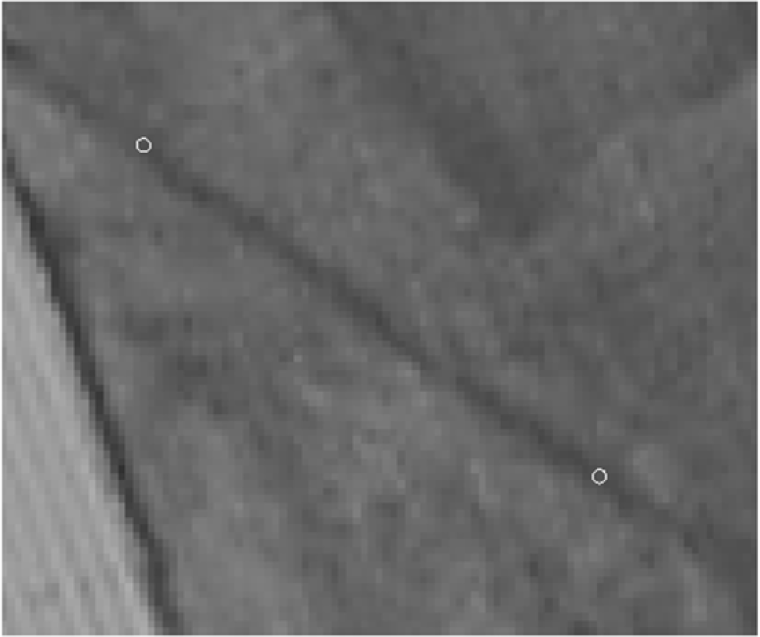
In Figure 1 an aerial image of an archaeological crop mark, visible on the ground in the area of Foggia (Italy), is reported. The presence of a significant wide line together with some other irrelevant information due to noise or vegetation changes is evident. The corresponding line profile, reported in Figure 2, demonstrates that the line cannot be characterized by a sharp and well-defined jump against a uniform background. This observations gave us the idea to modify an ANOVA based approach to consider the expected line shape and detect wide lines in noisy images comparing variances of neighbor regions.

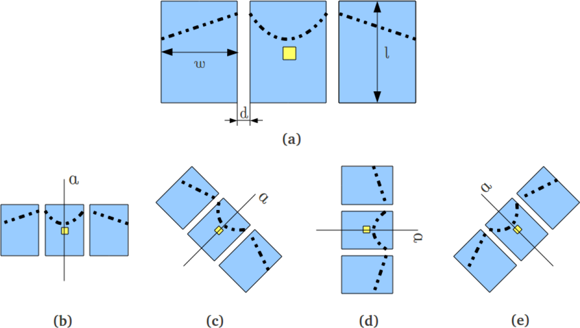
The presence of a line can be locally detected by searching for a pattern composed of three regions with different gray levels.

By comparing the gray levels of the populations of these three portions it is possible to determine if they belong to the same population (background). Therefore, for each pixel of the image we extract three parallel rectangular regions around it as shown in Figure 3a. These regions are finally rotated in four different directions, producing the results in Figure 3b,e). In these regions the modified ANOVA approach is applied.

The proposed algorithm works in the following way. The proposed modified ANOVA approach is applied for each point of the image and for any direction among those possible. Then, a t-test is applied on a contrast function that relates the parameters characterizing the three regions. A positive t-test answer means that the three regions belong to the same population (i.e., background region) and a new direction is considered. On the contrary, if t-test answer is negative, it is necessary to understand how much the difference between the three groups is due to the real presence of a line or is simply due to smooth background variations. For this reason the η² parameter is evaluated to measure the line effect size and decide if the considered point belongs to the line or to the background region.

The main contribution of the paper is the introduction of a modified ANOVA approach that uses a regression method to model the points belonging to the central area of the line with a second order polynomial function. On the contrary, the points belonging to the lateral regions are modelled by a first order polynomial functions. As well, the introduction of the parameter η² for the comparisons of statistics was done to make the final decision more indulgent or restrictive.

In the remaining part of this section we describe how the standard ANOVA approach was applied in our context, and the proposed modified ANOVA, together with the η² statistic test which was applied after the t-test to validate the membership of the point to a line or to a background region. The general formulation is finally tested to find more efficient models able to assist the ANOVA formulation.

2.1. The ANOVA Approach

The ANOVA is a widely used technique for separating the observed variance in a group of samples into portions which are traceable to different sources [43]. Thus the different samples may have undergone different treatments which affect the general level of the measured variate X. The variance analysis method enables us to estimate how much the variance is attributable to one cause and how much to the other and so to decide whether or not the treatments have produced any significant effects. The modelling of an image using treatments was introduced in [40,41]. The contribution of a treatment to a specified group of pixels is called a treatment effect.

Let x be the gray level of a pixel. If x_ij is the j-th measured value of x in the i-th region, then the mathematical model of ANOVA is

$$x_{ij}={\mu }_i+{\in }_{ij}$$

(1)

where for every i and j, ϵ_ij is normally distributed with expectation 0 and variance σ². This means that the measured x_ij for any individual pixel is made up of an effect due to the particular treatment undergone by the i-th region denoted by μ_i, and a random or error term ϵ_ij due to many unspecified causes. These ϵ_ij are supposed to be uncorrelated to each other. If we consider a problem with three samples, the null hypothesis is that the three groups belong to the same population with mean μ, that is

$$H_0:{\mu }_1={\mu }_2={\mu }_3=\mu$$

(2)

The ordinary statistic test of a one way-ANOVA can be used to infer whether to accept or reject the null hypothesis. If the three regions belong to different populations (they are produced by a source of variability, i.e., a treatment, such as the presence of a line), the null hypothesis is rejected.

Let us now consider the total sum of squared deviations (SS_T) of the whole area from the over-all mean $\overline{\mu }$: it can be divided in part due to the difference between the groups (SS_B) and in part due to the difference within the groups (SS_W ):

$${{\displaystyle \sum _{i,j}{(x_{i,j}-\overline{\mu })}^2=n_i{\displaystyle \sum _{i=1,2,3}{({\overline{\mu }}_1-\overline{\mu })}^2}+{\displaystyle \sum _{\begin{array}{c}i=1,2,3\\ j=1,\dots ,n_i\end{array}}(x_{i,j}-{\overline{\mu }}_i)}}}^2,$$

(3)

i.e., SS_T = SS_B + SS_W Note that n_i is the number of pixels of the i-th group. Then it is possible to observe that by straightforward calculations the mixed term vanishes:

$$2{\displaystyle \sum _{\begin{array}{c}i=1,2,3\\ j=1,\dots ,n\end{array}}({\overline{\mu }}_i-\overline{\mu })(x_{i,j}-{\overline{\mu }}_i)}=0$$

(4)

By dividing SS_B and SS_W by the correct number of degrees of freedom, respectively p − 1 and n_T − p, where n_T is the total number of pixels considered and p = 3 is the number of treatments, we get an estimation of the “variance between” and the “variance within”:

$$s_B^2=\frac{S{S}_B}{p-1}\text{and}\frac{S{S}_W}{n_T-p}$$

(5)

The ratio between the two variances is F-distributed, where F is the Fisher distribution:

$$\frac{s_B^2}{s_W^2}~F_{2,n_T-3}$$

(6)

At an α-level of significance, if the empirical value of F is greater than the critical value, we can reject the null hypothesis and assert that the three regions belong to different populations.

2.2. The Modified ANOVA

In order to have a consistent one-way ANOVA test, two important assumptions are necessary: normality of the distribution of gray levels of any pixel around the constant level μ_i and constancy of variance in the whole region. In ordinary cases, this assumption is quite restrictive because ridges or valleys, which are objects of investigation in the image, often show a well-defined shape. Pixel gray levels are strongly conditioned by the underlying profile, therefore we clearly commit significant errors in assuming the normality of pixels around constant values, rather than assuming normality around the shape profile. The estimation of the variance is affected by these errors and the homogeneity test fails.

In order to infer a more consistent statistical analysis, we properly reformulate (1) by taking into account the shape of the profile:

$$x_{i,j}=f_i(r_j,c_j)+{\in }_{i,j}$$

(7)

where the functions f_i : R² → R are surfaces describing the shape profile of the i-th region calculated in the coordinate row r_j and column c_j of a generic pixel of the image. The null hypothesis is the same as (2) but now this condition is transferred onto the parameters which characterize the functions f_i and not onto the means of the three regions. With reference to the real case reported in Figure 2, it is possible to admit that the pixel profiles in the three regions can be modelled using a quadratic surface, whose coefficients have to be determined in the least square sense, thus limiting the noise contribution which affects the image.

As a starting point of the modified ANOVA, a novel domain is defined around any pixel of the image. In this case, the domain is made of n_T discrete points, whose position is expressed by the two independent variables u and v. The two variables are referred to system of coordinates whose origin is in the center of the second region. Moreover, these variables spans uniformly within the limits of the three regions where the ANOVA method will be developed. Specifically, the first region is discretized in n₁ points having u and v spanning between $\left[-\frac{3w}{2},\frac{w}{2}\right]$ and $\left[-\frac{l}{2},\frac{l}{2}\right]$, respectively; the second region has n₂ points whose u and v coordinates spans between $\left[-\frac{w}{2},\frac{w}{2}\right]$ and $\left[-\frac{l}{2},\frac{l}{2}\right]$; equivalently, the third region of n₃ terms has a bounded domain where u and v changes between $\left[\frac{w}{2},\frac{3w}{2}\right]$, and $\left[-\frac{l}{2},\frac{l}{2}\right]$. Note that the boundaries of the external regions are here defined without any displacement. On the contrary, the displacement term shifts the first region by −d and the third region by d along the u-axis.

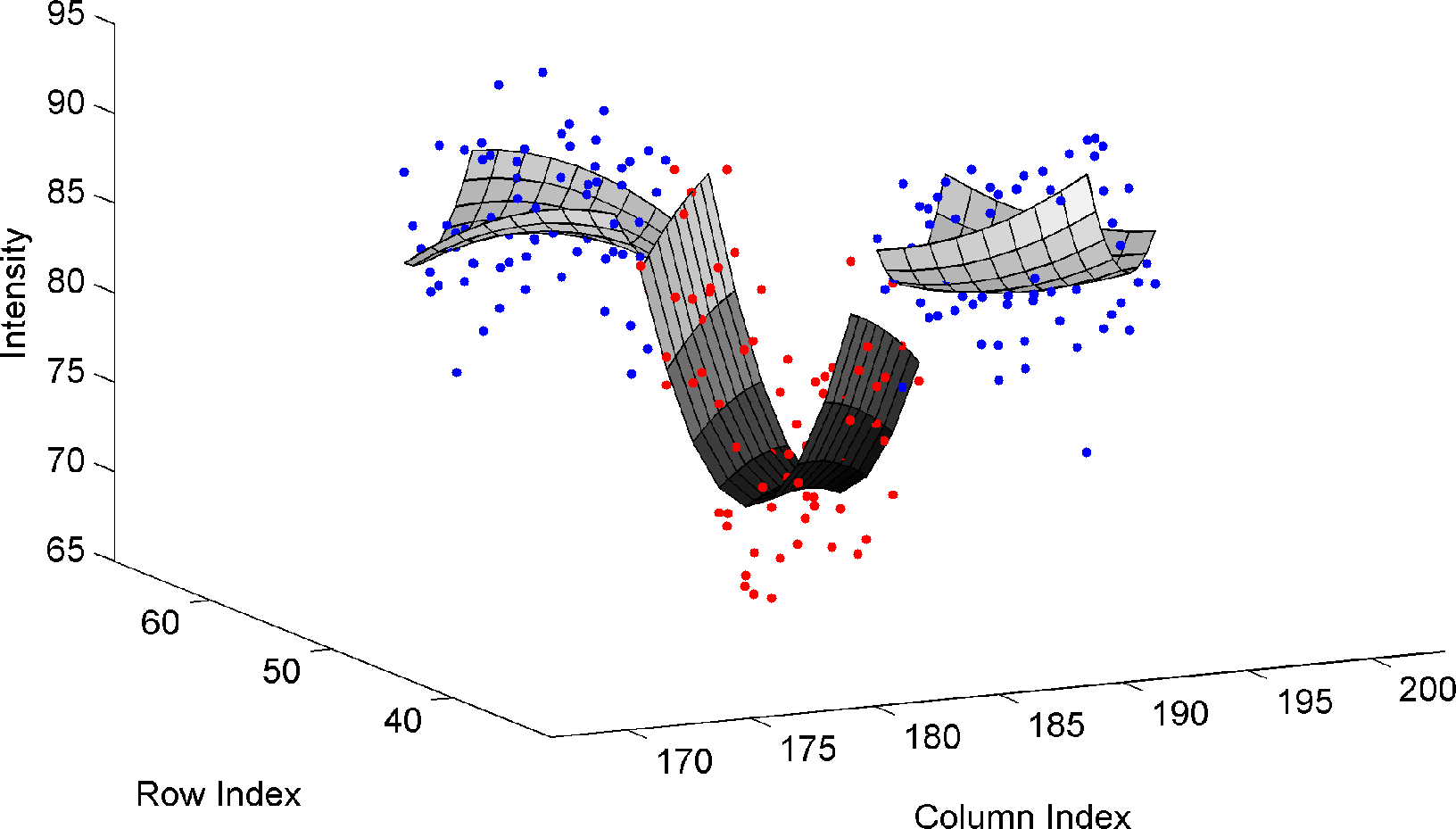
The domain has to be finally rotated accordingly with the specific α orientation considered for the ANOVA computation. Discrete coordinates are thus arranged in column vectors and multiplied by a proper two-dimensional rotation matrix. The resulting discrete coordinates represent the actual indices u_j and v_j, j = 1, …, n_T, where the pixel images can be extracted for the analysis of variances. Each point of the domain is projected on the surface generated by means of a bilinear interpolation on the intensity values of the image. This process produces three new vectors of pixel intensities, labelled as $Y_i={[y_{i,1},y_{i,2},\dots ,y_{i,n_i}]}^T$, where i is the index of the specific region under analysis. An example of 45°-oriented discrete domain is reported in Figure 4, together with the set of points of the vectors Y_i, extracted from the input data.

As stated before, the functions f_i can be represented as two-dimensional paraboloids whose formulations are straightforwardly equal to:

$$f_i(u,v)=a_{i,1}{u}^2+a_{i,2}{v}^2+a_{i,3}uv+a_{i,4}u+a_{i,5}v+a_{i,6}$$

(8)

whose average values in the corresponding range of existence of u and v, labelled as ${\overline{\mu }}_i$, are obtained easily by the application of the mean value theorem for integration:

$$\begin{array}{l}{\overline{\mu }}_1=\frac{13}{12}{a}_{1,1}{w}^2+\frac{1}{12}{a}_{1,2}{l}^2-a_{1,4}w+a_{1,6}\\ {\overline{\mu }}_2=\frac{1}{12}{a}_{2,1}{w}^2+\frac{1}{12}{a}_{2,2}{l}^2+a_{2,6}\\ {\overline{\mu }}_3=\frac{13}{12}{a}_{3,1}{w}^2+\frac{1}{12}{a}_{3,2}{l}^2+a_{3,4}w+a_{3,6}\end{array}$$

(9)

The parameters to be estimated are now expressed in terms of three vectors (A₁, A₂ and A₃), of six entries each. More specifically, each vector has the form A_i = [a_i,1, a_i,2, …, a_i,6]^T, and its entries can be obtained by applying the least squares method, given the input data in Y_i.

Let X_i be

$$X_i=\left[\begin{array}{cccccc}{u}_{i,1}^2& v_{i,1}^2& u_{i,1}{v}_{i,1}& u_{i,1}& v_{i,1}& 1\\ u_{i,2}^2& v_{i,2}^2& u_{i,2}{v}_{i,2}& u_{i,2}& v_{i,2}& 1\\ ⋮& ⋮& ⋮& ⋮& ⋮& ⋮\\ u_{i,n_i}^2& v_{i,n_i}^2& u_{i,n_i}{v}_{i,n_i}& u_{i,n_i}& v_{i,n_i}& 1\end{array}\right]$$

(10)

Then, by applying the least squares method we can estimate the unknown elements of the vectors A_i:

$$A_i={(X_i^T{X}_i)}^{-1}{X}_i^T{Y}_i$$

(11)

Figure 5 reports an example of the fitting paraboloids obtained by the least squared method applied on the data in Figure 4.

Let us consider again the total sum of squared deviations (SS_T ) of the whole area from the over-all mean $\overline{\mu }$ as in (3):

$$\begin{array}{l}{\displaystyle \sum _{i,j}{(y_{i,j}-\overline{\mu })}^2={\displaystyle \sum _{\begin{array}{c}i=1,2,3\\ j=1,\dots ,n_i\end{array}}{(f_i(u,v)-\overline{\mu })}^2}}\\ +{\displaystyle \sum _{\begin{array}{c}i=1,2,3\\ j=1,\dots ,n_i\end{array}}{(y_{i,j}-f_i(u,v))}^2}\end{array}$$

(12)

i.e., SS_T = SS_B + SS_W. It is still possible to prove that the mixed term

$$2{\displaystyle \sum _{\begin{array}{c}i=1,2,3\\ j=1,\dots ,n_i\end{array}}(f_i(u,v)-\overline{\mu })(y_{i,j}-f_i(u,v))=0}$$

(13)

The equations (5) still give an estimation of the “variance between” and the “variance within”.

In order to assert that the source of variability is a line, we have to compare the central region with the two adjacent ones, thus underlining a significant difference. It can be done by using the contrast function λ: ${ℛ}^3\to ℛ$defined as:

$$\lambda (\alpha ,\beta ,\gamma )=c_1\alpha +c_2\beta +c_3\gamma$$

(14)

where c_i ∈ R for any i = 1, 2, 3. We introduce the test parameter:

$$\overline{t}=\frac{\lambda ({\overline{\mu }}_1,{\overline{\mu }}_2,{\overline{\mu }}_3)}{s_{\lambda }}$$

(15)

where

$$s_{\lambda }^2=s_W^2{\displaystyle \sum _i\frac{c_i^2}{n_i}}$$

(16)

is an estimation of the variance of λ. In the null hypothesis, i.e., the contrast function calculated in the three means is zero, t follows a t-Student distribution with n_T − p degrees of freedom, i.e.,

$$\overline{t}~t_{n_T-p}$$

(17)

In order to have the central region darker than the external ones it must be

$${\overline{\mu }}_2<\min ({\overline{\mu }}_1,{\overline{\mu }}_3)$$

(18)

and, if we choose (c₁, c₂, c₃) = (1, −2, 1) the function $\lambda ({\overline{\mu }}_1,{\overline{\mu }}_2,{\overline{\mu }}_3)$ must be greater than 0.

Under this condition, it is possible to do a one-tailed test in order to verify the null hypothesis or to accept an alternative one. So, at a fixed level of significance, if the experimental parameter t is greater than the critical value, the null hypothesis is rejected.

2.3. η² Test

Whenever the t-test rejects the null hypothesis, it is mandatory to understand this results is due to the presence of a textured background in the image or to a real variation among the three regions. For this reason, we introduce another test to obtain a greater statistical evidence. This test, named as η², evaluates the statistical parameters in the following way:

$${\eta }^2=\frac{S{S}_B}{S{S}_T}$$

(19)

It takes values between 0 and 1 and it measures how much of the total variance is due to the subdivision of the whole region. It is indeed the coefficient of correlation between the whole area and a pattern composed by the three regions having the pixels with gray level profiles found by the fitting procedures (f₁, f₂, and f₃). In summary, the parameter η² permits a more accurate analysis to decide whether accept the line or not, so it represents the main test for the effective line detector.

2.4. Model Accuracy

Before going through the analysis of results, it is necessary to estimate the accuracy of the fitting model used for the representation of the input pixel intensities. As shown in Equation (8), the model approximates the pixel intensities as a 2D paraboloid. The model is implemented in the three regions where the ANOVA is computed, and it is defined to better detect lines and ridges with weak boundaries.

On the other hand, the specific nature of the problem of mark extraction from aerial images of archaeological sites can be exploited to downsize the problem, invoking simpler models. In particular it is possible to introduce three further kinds of function f_i, in addition to the one of Equation (8):

$$\begin{array}{l}{f}_i{(u,v)}^{(1^{st}ord)}=a_{i,1}^{(1^{st}ord)}u+a_{i,2}^{(1^{st}ord)}v+a_{i,3}^{(1^{st}ord)}\\ f_i{(u)}^{(2^{nd}ord)}=b_{i,1}^{(2^{nd}ord)}{u}^2+b_{i,2}^{(2^{nd}ord)}u+a_{i,3}^{(2^{nd}ord)}\\ f_i{(u)}^{(1^{st}ord)}=b_{i,1}^{(1^{st}ord)}u+b_{i,2}^{(1^{st}ord)}\end{array}$$

(20)

where functions are sorted in descending complexity order. In this case $f_i{(u,v)}^{(1^{st}ord)}$ is planar surface (first order model) in two dimensions. In addition, $f_i{(u)}^{(2^{nd}ord)}$ and $f_i{(u)}^{(1^{st}ord)}$are two different models of the second and first order, respectively. These functions are curves defined on a 1D domain, obtained by accumulating the image pixels on the discrete values assumed by the variable u. Note that the coefficients of the models are now labelled by the letter b to underline that they belong to a 1D model.

With reference to the actual sample data reported in Figure 4, the models have been tested to show their validity to fit the intensities of the pixels. For this purpose, we introduce the root mean square error (RMSE) between the actual observed values and those predicted by the estimator. Results obtained by the application of the four models are highlighted in

Table 1. RMSE obtained by the application of the four models used for the modified ANOVA.

	RMSE
	Region i = 1	Region i = 2	Region i = 3
$f_i{(u,v)}^{(2^{nd}ord)}$	3.223	3.61	3.181
$f_i{(u,v)}^{(1^{st}ord)}$	3.374	5.776	3.533
$f_i{(u)}^{(2^{st}ord)}$	3.345	3.659	3.552
$f_i{(u)}^{(1^{st}ord)}$	3.357	5.737	3.557

where the analysis is divided for the three regions.

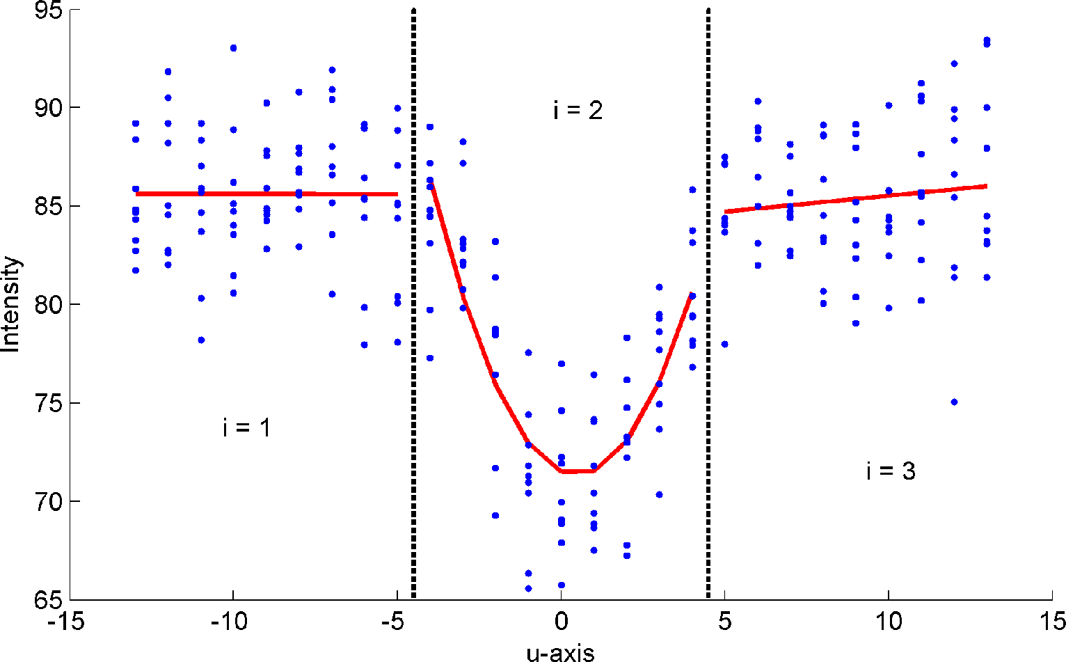
The inspection of Table 1 demonstrates a first important result: the internal region must be modelled by a second order function, since the RMSE are significantly lower than the ones obtained by the application of a first order function. This is due to the profile of the ridge to be detected within the image, which follows the shape of a parabola. On the contrary, the surrounding regions, i.e., the one addressed by the index i = 1, 3, can be modelled by a first order model, which induces a comparable RMSE with reference to those out of the second order models. Another aspect is even more important. The use of a 1D formulation of the domain, obtained by the projection of the span of the variable v on the u-axis, is enough to fit the input intensities. This result can be understood by looking at the surface in Figure 4. If the length l of the windows is not large, the three regions can be considered homogeneous in the longitudinal direction, so we can use a 1D profile to model the pixels of each region. As a consequence, the pixel intensities of the two external regions are distributed around straight lines, whereas the central region shows a parabolic profile along the longitudinal direction, defined by the u-axis.

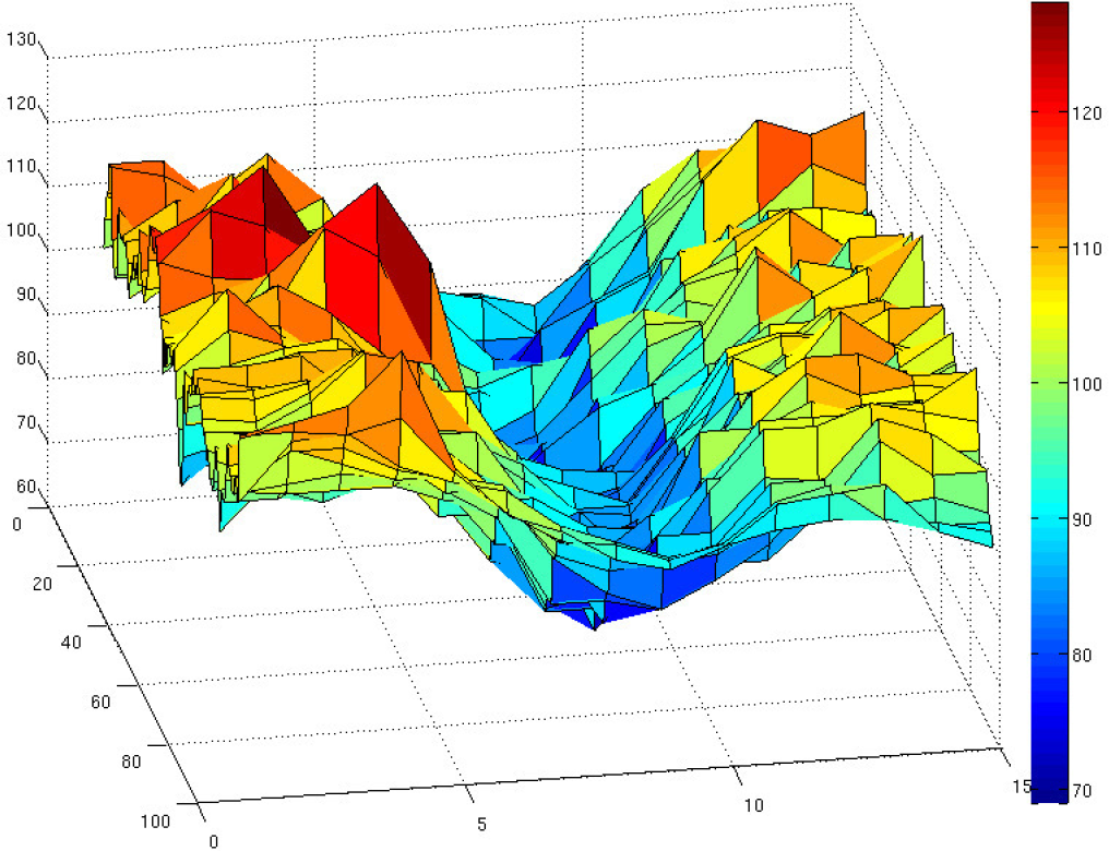
In Figure 6, the plot of the pixel intensity values makes the argued behavior more evident. In particular, the normality of the central region around a parabolic shape is surely more evident than around an ordinary mean value.

In summary, the fitting model for the approximation of the pixel intensities used in the Equation (12) of the modified ANOVA can be simplified, without altering the final results, but gaining efficiency. As a consequence, the final formulation can be expressed in seven parameters of the coefficient vectors ( $B_1={[b_{1,1}^{(1^{st}ord)},b_{1,2}^{(1^{st}ord)}]}^T$, $B_2={[b_{2,1}^{(2^{nd}ord)},b_{2,2}^{(2^{nd}ord)},b_{2,3}^{(2^{nd}ord)}]}^T$ and $B_3=[b_{3,1}^{(1^{st}ord)},b_{3,2}^{(1^{st}ord)}]$). Moreover, the three average values of the fitting functions, used in in Equation 12, are now expressed as:

$$\begin{array}{l}{\overline{\mu }}_1=-b_{1,1}^{(1^{st}ord)}w+b_{1,2}^{(1^{st}ord)}\\ {\overline{\mu }}_2=\frac{1}{12}{b}_{2,1}^{(2^{nd}ord)}w+b_{2,3}^{(2^{nd}ord)}\\ {\overline{\mu }}_3=b_{3,1}^{(1^{st}ord)}w+b_{3,2}^{(1^{st}ord)}\end{array}$$

(21)

Experiments on images will be finally performed using the simplified model proposed, thus giving more efficiency to the modified ANOVA formulation.

3. Experimental Results

In order to demonstrate performances it is necessary to establish a measure for the objective and quantitative evaluation of the line detection results. As affirmed in [44], the performance measures with quantitative analysis can be done when ground truth values are available. This is certainly possible with synthetic images. In natural images the ground truth is generated by humans who can provide various perfect solutions, since different humans might create discrepant interpretations. For these reasons, in this paper different sets of experiments were carried out to demonstrate performances: in the first set, quantitative tests on synthetic images with different curve typologies and various noise levels are described. In the second set of experiments, a real data set of images was used and qualitative comparative results with state of the art approaches are provided.

3.1. Synthetic Images

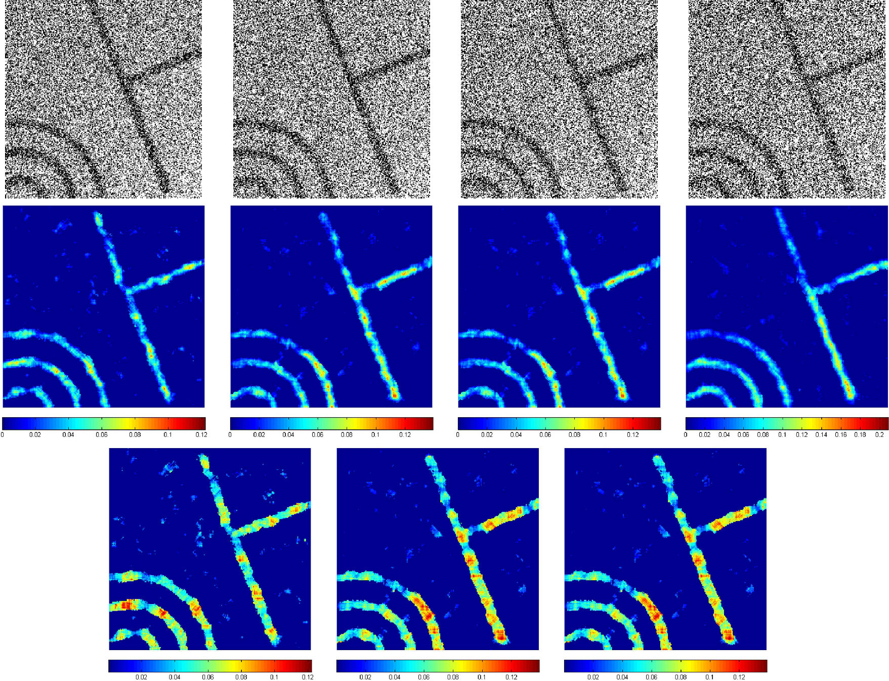
In order to estimate the detector’s efficiency, synthetic images corrupted by different noise levels were considered. The image contains several circles (with different radii) and two intersecting straight lines. Four standard deviation of noise distribution were considered with σ = 0.45, σ = 0.55, σ = 0.65, σ = 0.75. In the first row of Figure 7 the sample images are reported. The image dimension is 250×250, the lines have a 13-pixel-wide transversal section and have been modelled with a parabolic shape. For each point of the image we consider three windows, as reported in Figure 3, having a width w = l = 13 pixels and a displacement d = 1. On these three regions we applied the ordinary ANOVA as described in Equation (3), and the modified ANOVA described in Equation (12). Then, the t-test, described in Equation (15), was applied on the contrast function to evaluate whether the central region shows a mean value lower than those of the two adjacent ones. The significance level for the t-test of both methods was fixed to 0.01. In case of failure, the null hypothesis is rejected and the η² statistic is evaluated. In the second and third rows of Figure 7 the final results of the ordinary and modified methods are reported. Colors represent detections as the η² parameter changes. It is clear that the new way to estimate region variances fitting a shape model makes the modified method more sensitive than the ordinary one: comparing the results with equal η² parameters, the modified method has greater capability to detect more points of the lines.

In order to evaluate the performances, quantitative tests were carried out by the evaluation of

$$sensitivity=\frac{TP}{TP+FN}$$

(22)

$$accuracy=\frac{TP+TN}{TP+FP+FN+TN}$$

(23)

where TP, TN, FP and FN are, respectively, the number of True Positive, True Negative, False Positive and False Negative. The sensitivity is the ratio of the correctly detected line pixels over the total number of pixels labelled as line. If the method finds few False Negative the sensitivity reaches high values and indicates a high number of pixels correctly classified as lines. The accuracy is the fraction of all pixels which are correctly classified.

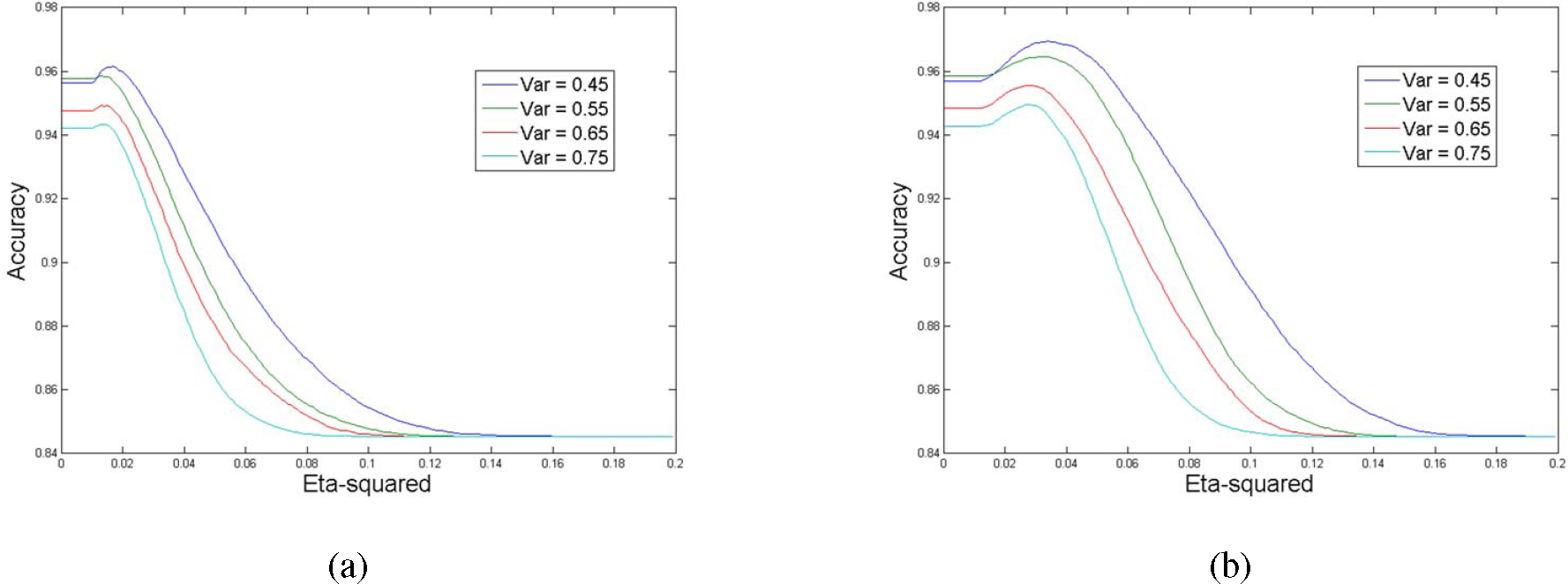
In Figure 8, the graphs of the accuracy variation as the η² parameter changes are reported. As explained before, the η² test is evaluated only on those points which did not satisfy the null hypothesis. So the t-test has a preprocessing role of eliminating all the background points which have clear evidence of belonging to the same background population. When small values of the η² parameters are used, the statistical test is no longer selective and all the points that passed the previous t-test contribute to the evaluation of the method’s accuracy. This consideration explains why, in the two graphs, the performances are assessed around constant values in the range 94%–96% when η² is under 0.02. When the η² parameter increases, the methods become more selective. For the modified ANOVA, if the η² parameters is chosen under the value 0.04, accuracy remains over the 95%. In

Table 2. Ordinary and modified ANOVA: sensitivity and accuracy values evaluated on the four synthetic images.

	η2 = 0.01
	ordinary	ANOVA	modified	ANOVA
	Acc.	Sens.	Acc.	Sens..
Image1	95.63%	84.45%	95.70%	84.94%
Image2	95.76%	81.50%	95.85%	82.15%
Image3	94.75%	76.19%	94.84%	76.87%
Image4	94.21%	73.57%	94.26%	74.05%
	η2 = 0.03
	ordinary	ANOVA	modified	ANOVA
	Acc.	Sens.	Acc.	Sens.
Image1	94.63%	66.97%	96.88%	84.41%
Image2	93.44%	58.59%	96.44%	81.03%
Image3	92.31%	50.86%	95.53%	73.95%
Image4	91.18%	43.55%	94.92%	70.50%
	η2 = 0.05
	ordinary	ANOVA	modified	ANOVA
	Acc.	Sens.	Acc.	Sens.
Image1	91.05%	42.27%	96.26%	78.03%
Image2	89.13%	29.72%	95.32%	71.39%
Image3	88.06%	22.77%	93.22%	57.56%
Image4	86.42%	12.16%	91.62%	46.99%

the detection results of the two methods are compared with the same η² parameters in terms of accuracy and sensitivity. With small values of the η² parameter (i.e., 0.01), the results of the two methods are comparable since they fall into the case of using only the t-test statistics, as explained above. When greater values are considered the modified method is more sensible and greater percentages of lines are correctly detected.

In order to evaluate the detection capability of the modified ANOVA when different window and spacing dimensions are used, a further experiment was performed. We considered different window dimensions in the set {9, 11, 13, 15, 17} and different spacings in the set {0, 2, 4, 6}. The considered line dimension is 13 pixels. In

Table 3. Modified ANOVA: sensitivity and accuracy values evaluated on the four synthetic images with varying window and spacing dimensions.

	Region Dimension: 17 × 17 (w = l = 17)
	Spacing: d = 0		Spacing: d = 2		Spacing: d = 4		Spacing: d = 6
	Acc.	Sens.	Acc.	Sens.	Acc.	Sens.	Acc.	Sens.
Image1	96.31%	89.62%	95.73%	89.21%	94.95%	87.27%	94.30%	84.80%
Image2	96.24%	89.65%	95.66%	86.20%	95.03%	84.28%	94.52%	81.68%
Image3	94.98%	75.92%	94.62%	76.24%	93.96%	75.07%	93.28%	72.39%
Image4	94.53%	71.30%	94.45%	71.99%	94.08%	70.81%	93.67%	68.68%
	Region Dimension: 15 × 15 (w = l = 15)
	Spacing: d = 0		Spacing: d = 2		Spacing: d = 4		Spacing: d = 6
	Acc.	Sens.	Acc.	Sens.	Acc.	Sens.	Acc.	Sens.
Image1	97.35%	89.63%	96.92%	91.24%	96.39%	90.76%	95.79%	88.93%
Image2	97.12%	86.84%	96.74%	88.65%	95.37%	88.42%	95.81%	86.50%
Image3	96.02%	78.17%	95.92%	80.25%	95.55%	80.13%	95.07%	79.30%
Image4	95.54%	74.30%	95.57%	76.83%	95.34%	76.82%	95.01%	75.56%
	Region Dimension: 13 × 13 (w = l = 13)
	Spacing: d = 0		Spacing: d = 2		Spacing: d = 4		Spacing: d = 6
	Acc.	Sens.	Acc.	Sens.	Acc.	Sens.	Acc.	Sens.
Image1	96.88%	84.41%	97.21%	88.75%	96.95%	90.88%	96.49%	90.50%
Image2	96.44%	81.03%	96.94%	85.79%	96.78%	88.19%	96.45%	87.54%
Image3	95.53%	73.95%	95.97%	78.09%	96.08%	81.00%	95.77%	81.06%
Image4	94.92%	70.50%	95.48%	75.06%	95.76%	78.27%	95.56%	78.24%
	Region Dimension: 11 × 11 (w = l = 11)
	Spacing: d = 0		Spacing: d = 2		Spacing: d = 4		Spacing: d = 6
	Acc.	Sens.	Acc.	Sens.	Acc.	Sens.	Acc.	Sens.
Image1	94.34%	71.81%	95.62%	80.44%	96.10%	84.98%	96.06%	87.28%
Image2	94.01%	67.45%	95.46%	76.78%	96.08%	81.85%	96.16%	84.25%
Image3	93.36%	63.21%	94.61%	71.47%	95.10%	75.91%	95.26%	78.03%
Image4	92.60%	60.10%	93.77%	67.82%	94.46%	72.47%	94.94%	75.70%
	Region Dimension: 9 × 9 (w = l = 9)
	Spacing: d = 0		Spacing: d = 2		Spacing: d = 4		Spacing: d = 6
	Acc.	Sens.	Acc.	Sens.	Acc.	Sens.	Acc.	Sens.
Image1	91.95%	59.34%	93.29%	68.13%	94.43%	76.09%	94.99%	79.90%
Image2	91.80%	56.72%	93.09%	64.54%	94.38%	72.75%	94.97%	76.76%
Image3	91.31%	52.82%	92.43%	59.81%	93.60%	67.54%	94.01%	71.20%
Image4	90.18%	48.66%	91.54%	56.70%	92.75%	64.19%	93.20%	67.63%

the results are reported. In bold the best results are highlighted. Due to the presence of noise in the four considered images a window dimension larger than the actual line dimension provides higher performances as a larger number of points contribute to the statistics. In fact with a window of 15 pixels and no spacing among the regions the highest performances were obtained in almost all the cases. When smaller windows are considered the best performances are reached when the sum between the window dimension and the spacing is around 15 pixels. These considerations can be used to select the w and d parameters needed in the proposed methodology. If the images have a low noise level, the window dimensions can be selected as the same dimensions as the searched lines, but when there is a low contrast and a high level of noise, it would be better to use a larger window with a small spacing to allow more points to contribute to the region statistics. If the image contains more lines with different widths, the method can be iterated from a small window dimension up to larger windows to detect all the possible lines of interest. In the following experiments on real images, we use these considerations to set the parameters and perform comparisons with other detection approaches.

3.2. Real Images

In order to demonstrate the general applicability of the proposed method, experiments carried out on real images of crop marks and comparisons with state-of-the-art approaches are provided in this section. Since the proposed method detects the whole line, we selected two methods among the related literature on wide line detectors: an active contour based approach proposed in [37], and a wide line detection technique based on an isotropic nonlinear filtering (proposed in [31]). Since lines can be extracted by applying methods that use edge information, the results provided by the Canny method [17] are also reported, as it is considered by the related literature [44] one of the methods that produces optimal solutions.

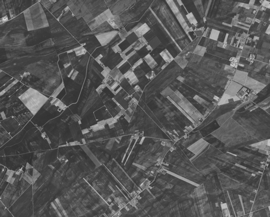
Figure 9 shows a real image acquired using a digital aerial pushbroom scanner ADS40 by Leica Geosystems [45] in the Apulia Tavoliere. The pushbroom scanner is made of 8 parallel linear CCD sensors, of 12,000 pixels each, having size of 6.5 μm. The sensor is able to produce orthoimages whose width is equal to 24,000 pixels, since two arrays of CCD elements are shifted each other by 0.5 pixel. Given the focal length of 62.5 mm and the distance of the sensor from the ground (20, 500ft), the spatial resolution is close to 560 mm, depending on the morphology of the scanned area. Finally, the radiometric resolution is converted from the initial 16 bits per channel to 8 bits per channel. The smallest image produced by the scanner has the size of the Italian topographic regional maps (Carta Tecnica Regionale, CTR) and covers an area of about 7.4 × 6.6 km, which corresponds to an image of 14, 800×11, 840 pixels. Then, the resulting images are divided in smaller pictures, having size 600×500 pixels. A sample picture is reported in Figure 10a, where some relevant archaeological crop marks are annotated as tombs and Neolithic walls by expert archaeologists. The results obtained with the Canny edge detection approach and the modified Active Contour approach are reported in Figure 10b,c. As the image contains a lot of non-relevant data (such as signs of plowing, trees, and so on) together with significant archaeological traces, the edge information (even with a possible postprocessing) cannot be directly used. The Active contour approach requires an ad-hoc initialization process to select some seed points on the interesting marks (see the green points in Figure 10c), and it suffers when the crop marks present some discontinuities that interrupt the growth of the active contours. The results obtained with the isotropic nonlinear filtering and the proposed approach are reported in Figure 10d,e. The proposed approach was applied with a window dimension of 5 × 11 pixels, spacing d = 2 pixels, and η² = 0.45. The results of the isotropic nonlinear filtering were the best ones obtained choosing the parameter t = 6 and the radius of the circular mask r = 21 (see Ref. [31] for further explanations). In order to avoid small regions, all results reported in Figure 10 are obtained after a morphological closing of one pixel, and the suppression of connected regions with a small area (under 50 pixels). In this way, the application of the same post-processing deletes possible sources of error, thus improving equivalently the overall outcomes. The results obtained by the proposed approach are shown in Figure 10e and are easily interpretable: unbroken long lines are detected with high accuracy. In terms of artifacts, the resulting image contains few regions that can be due to the presence of noise or to irrelevant signs of crops.

Further processing of the orthoimages of the area of the Apulian Tavoliere have been performed, leading to the results of Figure 11. In this case, according to the resolution of the images (a pixel corresponds to a ground area of 500 mm) and the width of the objective marks (close to 1 m), the mask dimensions for the treatment analysis have been set equal to w = 3 and l = 5, whereas the statistical parameter η² is equal to 0.6. Outcomes clearly prove that the η² test is able to effectively highlight only those image pixels which actually belong to significant crop marks, keeping out the detection of possible lines of the ground pattern.

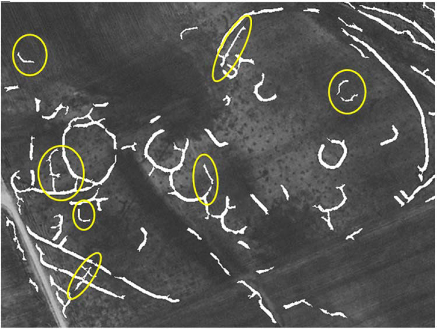
On the other hand, the main limitation of the proposed approach is the dependence between the line width and the total window dimension (i.e., w + d). Large windows may preclude the detection of lines with a width much lower than the window size. However, the proposed approach can be iterated more times using different window sizes. Figure 12 reports the result obtained on the aerial image of Figure 10a by iterating two times the proposed approach with the same window dimension but with two different spacings d = 2 and d = 0 pixels. The yellow circles highlight the areas in which finer lines were detected. In this case, it is evident that an higher number of archaeological traces are detected, without introducing false positives.

4. Conclusions

In this paper we propose a wide line detection approach for the extraction of archaeological crop marks that uses the analysis of variance to decide if a point belongs to a mark or to the background. The method has been applied to process large aerial images and provide to the archaeologists a set of candidate regions which probably correspond to un-excavated archaeological sites. The knowledge of the expected appearance of crop marks has been used to modify the ANOVA approach and provide a more selective wide line detection approach. In order to decide if a point belongs to a line three regions around this point are considered and the variance with respect to a fitted shape model is evaluated. The η² statistics is estimated on the variances among these regions to make the final decision. Different experiments on synthetic and real images demonstrate the performances of the proposed approach with respect to assessed state-of-the-art methodologies. The introduction of the regression analysis to fit the shape model in each region allows for a more precise evaluation of the variances taking into account the expected shape of the searched lines. The use of the η² parameter allows users to modify the required sensibility at the end of the detection process. Future work will address the introduction of different models with polynomials of higher orders or with more general functions, in order to extend the concepts of the modified ANOVA to the detection of different patterns, related to traces with complex shapes.

References

- Jaynes, C.; Riseman, E.; Hanson, A. Recognition and Reconstruction of Nuiling from Multiple Aerial Images; Computer Vision and Image Undestranding; 2003; Volume 90, pp. 68–98. [Google Scholar]
- Verhoeven, G.J. Near-Infrared aerial crop mark archaeology: From its historical use to current digital implementations. J. Archaeol. Method Theory. 2012, 1, 132–160. [Google Scholar]
- Lasaponara, R.; Masini, N. Beyond modern landscape features: New insights in the archaeological area of Tiwanaku in Bolivia from satellite data. Int. J. Appl. Earth Observ. Geoinf. 2014, 26, 464–471. [Google Scholar]
- Lasaponara, R.; Masini, N. Detection of archaeological crop marks by using satellite QuickBird multispectral imagery. J. Archaeol. Sci. 2007, 34, 214–221. [Google Scholar]
- Agapiou, A.; Alexakis, D.; Sarris, A.; Hadjimitsis, D. Orthogonal equations of multi-spectral satellite imagery for the identification of un-excavated archaeological sites. Remote Sens. 2013, 5, 6560–6586. [Google Scholar]
- Aqdus, S.A.; Hanson, W.S.; Drummond, J. Finding archaeological cropmarks: A hyperspectral approach. Proc. SPIE 2007, 6749. [Google Scholar] [CrossRef]
- Chen, F.; Masini, N.; Yang, R.; Milillo, P.; Feng, D.; Lasaponara, R. A space view of radar archaeological marks: First applications of COSMO-SkyMed X-band data. Remote Sens. 2015, 7, 24–50. [Google Scholar]
- Luo, L.; Wang, X.; Guo, H.; Liu, C.; Liu, J.; Li, L.; Du, X.; Qian, G. Automated extraction of the archaeological tops of qanat shafts from VHR imagery in google earth. Remote Sens. 2014, 6, 11956–11976. [Google Scholar]
- Scott, D.; Boyd, D.; Beck, A.; Cohn, A. Airborne LiDAR for the detection of archaeological vegetation marks using biomass as a proxy. Remote Sens. 2015, 7, 1594–1618. [Google Scholar]
- Doneus, M.; Verhoeven, G.; Atzberger, C.; Wess, M.; Rus, M. New ways to extract archaeological information from hyperspectral pixels. J. Archaeol. Sci. 2014, 52, 84–96. [Google Scholar]
- Atzberger, C.; Wess, M.; Doneus, M.; Verhoeven, G. ARCTIS—A MATLAB toolbox for archaeological imaging spectroscopy. Remote Sens. 2014, 6, 8617–8638. [Google Scholar]
- Mueller, M. Edge- and region-based segmentation technique for the extraction of large, man-made objects in high-resolution satellite imagery. Pattern Recognit. 2004, 37, 1619–1628. [Google Scholar]
- Fradkin, M.; Maitre, H.; Roux, M. Building detection from multiple aerial images in dense urban areas. Comput. Vis. Image Underst. 2001, 83, 181–207. [Google Scholar]
- Jaynes, C.; Riseman, E.; Hanson, A. Recognition and reconstruction of building from multiple aerial images. Comput. Vis. Image Underst. 2003, 90, 68–98. [Google Scholar]
- Wang, Y.; Tupin, F.; Han, C. Building detection from high resolution PolSAR data at the rectangle level by combining region and edge information. Pattern Recognit. Lett. 2010, 31, 1077–1088. [Google Scholar]
- Gautama, S.; Goeman, W.; Haeyer, J.D.; Philips, W. Characterizing the perfor mance of automatic road detection using error propagation. Image Vis. Comput. 2006, 24, 1001–1009. [Google Scholar]
- Canny, J. A Computational Approach to Edge Detection. IEEE Trans. Pattern Anal. Mach. Intell. 1986, 8, 679–698. [Google Scholar]
- Moon, H.; Chellappa, R. A rosenfeld, optimal edge-based shape detection. IEEE Trans. Image Process. 2002, 11, 1209–1227. [Google Scholar]
- Pellegrino, F.A.; Vanzella, W.; Torre, V. Edge detection revised. IEEE Trans. Syst. Man Cybern. Part B: Cybern. 2004, 34, 1500–1518. [Google Scholar]
- Yu, Y.; Acton, S.T. Edge detection in ultrasound imagery using the instantaneous coefficient of variation. IEEE Trans. Image Process. 2004, 13, 1640–1655. [Google Scholar]
- Rakesh, R.R.; Chaudhuri, P.; Murthy, C.A. Thresholding in edge detection: A statistical approach. IEEE Trans. Image Process. 2004, 13, 927–936. [Google Scholar]
- Duda, R.O.; Hart, P.E. Use of the Hough Transformation to Detect Lines and Curves in Pictures; Comm. ACM: New York, NY, USA, 1972; Volume 15, pp. 11–15. [Google Scholar]
- Illingworth, J.; Kittler, J. A survey of the Hough transform. Comput. Vis. Graph. Image Process. 1988, 44, 87–116. [Google Scholar]
- Leavers, V.F. Which Hough transform? CVGIP Image Underst. 1993, 58, 250–264. [Google Scholar]
- Ballard, D.H. Generalizing the Hough transform to detect arbitrary shapes. Pattern Recognit. 1981, 13, 111–122. [Google Scholar]
- D’Orazio, T.; Leo, M.; Guaragnella, C.; Distante, A. A visual approach for driver inattention detection. Pattern Recognit. 2004, 40, 2341–2355. [Google Scholar]
- Li, Z.; Liu, Y.; Walker, R.; Hayward, R.; Zhang, J. Toward automatic power line detection for a UAV surveillance system using pulse coupled neural filter and an improved Hough transform. Mach. Vis. Apll. 2010, 21, 677–686. [Google Scholar]
- D’Orazio, T.; Guaragnella, C.; Leo, M.; Distante, A. A new algorithm for ball recognition using circle Hough tranform and neural classifier. Pattern Recognit. 2004, 37, 393–408. [Google Scholar]
- Lu, W.; Tan, J. Detection of incomplete ellipse in images with strong noise by iterative randomized Hough Transorf (IRHT). Pattern Recognit. 2008, 41, 1268–1279. [Google Scholar]
- Liu, L.; Zhang, D.; You, J. Detecting wide lines using isotropic nonlinear filtering. IEEE Trans. Image Process. 2007, 16, 1584–1595. [Google Scholar]
- Koller, T.M.; Gerig, G.; Szekely, G.; Dettwiler, D. Multiscale detection of curvilinear structures in 2-D and 3-D image data, Proceedings of the 5th International Conference on Computer Vision, Boston, MA, USA, 20–23 June 1995; pp. 864–869.
- Steger, C. An unbiased detector of curvilinear structures. IEEE Trans. Pattern Anal. Mach. Intell. 1998, 20, 113–125. [Google Scholar]
- Chan, T.F.; Vese, L.A. Active contours without edges. IEEE Trans. Image Process. 2001, 10, 266–277. [Google Scholar]
- Kass, M.; Witkin, A.; Terzopolulos, D. Snakes: Active contour model. Int. J. Comput. Vis. 1988, 1, 321–331. [Google Scholar]
- Caselles, V.; Kimmel, R.; Sapiro, G. Geodesic active contour. Int. J. Comput. Vis. 1997, 22, 61–79. [Google Scholar]
- D’Orazio, T.; Palumbo, F.; Guaragnella, C. Archaeological trace extraction by a local directional active contour approach. Pattern Recognit. 2012, 45, 3427–3438. [Google Scholar]
- Lankton, S.; Tannenbaum, A. Localizing region-based active contours. IEEE Trans. Image Process. 2008, 17, 2029–2039. [Google Scholar]
- Darolti, C.; Mertins, A.; Bodensteiner, C.; Hofmann, U. Local region descriptors for active contour evolution. IEEE Trans. Image Process. 2008, 17, 2275–2288. [Google Scholar]
- Genello, G.; Cheung, J.; Billis, S.; Saito, Y. Gaeco-Latin squares design for line detection in the presence of correlate noise. IEEE Trans. Image Process. 2000, 9, 609–622. [Google Scholar]
- Behar, D.; Cheung, J.; Kurz, L. Contrast techniques for line detection in correlated noise environmnt. IEEE Trans. Image Process. 1997, 6, 625–641. [Google Scholar]
- Xue, J.H.; Titterington, D.M. t-test, F-test and Otsu’s methods for image thresholding. IEEE Trans. Image Process. 2011, 20, 2392–2396. [Google Scholar]
- Keeping, E.S. Introduction to Statistical Inference; Dover Pubblication, Inc.: New York, NY, USA, 1995. [Google Scholar]
- Lopez-Molina, C.; de Baets, B.; Bustince, H. Quantitatve error measures for edge detection. Pattern Recognit. 2013, 46, 1125–1139. [Google Scholar]
- Sandau, R.; Braunecker, B.; Driescher, H.; Eckardt, A.; Hilbert, S.; Hutton, J.; Kirchhofer, W.; Lithopoulos, E.; Reulke, R.; Wicki, S. Design principles of the LH Systems ADS40 airborne digital sensor. Int. Arch. Photogramm. Remote Sens. 2000, 33, 258–265. [Google Scholar]