Detecting Clear-Cuts and Decreases in Forest Vitality Using MODIS NDVI Time Series

Abstract

This paper examines the potential of MODIS-NDVI time series for detecting clear-cuts in a coniferous forest stand in the south of France. The proposed approach forms part of a survey monitoring the status of forest health and evaluating the forest decline phenomena observed over the last few decades. One of the prerequisites for this survey was that a rapid and easily reproducible method had to be developed that differentiates between forest clear-cuts and changes in forest health induced by environmental factors such as summer droughts. The proposed approach is based on analysis of the breakpoints detected within NDVI time series, using the “Break for Additive Seasonal and Trend” (BFAST) algorithm. To overcome difficulties detecting small areas on the study site, we chose a probabilistic approach based on the use of a conditional inference tree. For model calibration, clear-cut reference data were produced at MODIS resolution (250 m). According to the magnitude of the detected breakpoints, probability classes for the presence of clear-cuts were defined, from greater than 90% to less than 3% probability of a clear-cut. One of the advantages of the probabilistic model is that it allows end users to choose an acceptable level of uncertainty depending on the application. In addition, the use of BFAST allows events to be dated, thus making it possible to perform a retrospective analysis of decreases in forest vitality in the study area.

1. Introduction

Due to the long life of woody species and the rate of climate change, European forest ecosystems are particularly sensitive to climate change, especially to extreme climatic events [1]. Depending on the local conditions and on the species of tree, these phenomena can cause a decline in forest health [2,3]. The assessment of the impacts of climate change on forest ecosystems is a real challenge for the scientific community [4].

Long-term observations highlight the changes in forest ecosystems. Three main types of change are defined [5]: gradual changes usually driven by climate change, caused by gradual degradation of the environment; phenological or seasonal changes, corresponding to phenological modifications such as shifts in growing season [6]; and abrupt changes related to disturbances such as deforestation or forest fires [7,8]. Declining forest health can be characterized by a gradual decrease in activity or sometimes by an abrupt decrease in activity caused by extreme climatic events such as intense summer drought or by a pathogen attack. Other events may also cause abrupt changes of activity within stands such as clear-cutting or thinning, whether or not these are related to any decline in forest health.

In France, coniferous stands of major economic interest have been particularly affected by climatic conditions over the last decade. In this context, there is a need to monitor the status of forest health and detect any decreases in vitality in order to support new forestry management practices and strategies. Coniferous stands in the south of the French Massif Central Mountains were severely affected by a summer drought in 2003. Forest decline was observed for a few years after this climatic event, corresponding to significant loss of vitality, leading to tree mortality. Vegetation indices, such as the Normalized Difference Vegetation Index (NDVI), are frequently used to monitor vegetation thanks to their close link with the primary production of vegetation [9,10,11]. A method based on the analysis of NDVI satellite image time series was developed in a previous study [12,13,14] to evaluate the phenomenon of decline throughout the whole forest area. Furthermore, the relevance of the use of a spring greenness indicator was validated by comparison with a ground-level tree vitality indicator. However, this method did not make it possible to distinguish between a negative trend in this indicator related to a decrease in forest vitality or one related to a clear-cut. To locate, quantify and monitor the evolution of declining stands, it is essential to distinguish them from stands impacted by forestry practices. The work presented here aims to deal with this issue by proposing a method for detecting clear-cuts, based on a probabilistic approach.

The detection of deforestation or forest clear-cuts using coarse resolution images is generally difficult because of the patchy patterns of impacted areas [15]. The accuracy of the results usually depends on the magnitude of the signal, the size of the area undergoing change and the degree of forest stand fragmentation [16]. Several authors have suggested methods for detecting clear-cuts or deforestation using coarse spatial resolution (e.g., 250–1000 m) satellite data [17,18]. These detection methods are based on changes in spectra or in texture between two dates. These authors highlighted that methods based on changes in texture were the least accurate. Clear-cuts that extend over less than 15 ha are difficult to detect due to the high number of errors of commission [17]. Morton et al. reported that the most appropriate method for detecting clear-cuts using MODIS images depends on what the user needs [19]. These may go from the need to detect all impacted areas with significant errors of commission to a need for a more accurate detection of clear-cut areas with significant errors of omission. Detection methods can be based on the binary “change—no change” classification [17,18] or probabilistic approaches [16,20]. Probabilistic approaches have some advantages over binary change methods because users can select the appropriate threshold according to their needs [21]. B. Desclée et al. showed the highest accuracy in detecting clear-cuts using high spatial resolution images (SPOT HRV) [22]. Recently, a large number of authors have simultaneously used MODIS and Landsat images to improve the detection of forest disturbances [23,24,25].

MODIS data actually have a spatial resolution that is not optimal for our study area, but they are most suitable for some essential requirements already stated, such as (a) the development of easily renewable methods that do not require major computing resources; (b) the availability and cost-free nature of the products used and (c) regular data acquisition over large areas [26].

Although high spatial resolution images, such as Landsat TM or SPOT HRV, have a spatial resolution more appropriate to the size and shape of the studied stands, their availability is not suited to monitoring vegetation dynamics, as acquisition time regularity is usually limited by the satellites’ characteristics and cloud cover [27]. Moreover, considering Landsat and SPOT images and their archives, they are technically and financially difficult to mobilize in France. For regional applications, the cost and difficulties associated with the detection of disturbances on a regular basis could hinder the monitoring of forest stands [28].

Considering these limitations and the use made in the past of MODIS images to assess forest decline in our study area [14], we focused on exploring the potential of MODIS images for detecting clear-cuts.

The goal of this study is to propose a method based on change analysis that is suitable for mapping clear-cut areas and dating events using MODIS NDVI time series. Given the spatial resolution of the images, the high fragmentation of the stands concerned and the heterogeneity in the size of the clear-cuts in the study area, the proposed method is based on a probabilistic approach rather than a binary approach. Ultimately, this information is expressed as different clear-cut probability levels and should be used to complement a map of forests displaying the loss of vitality, which can be generated using the same MODIS image time series.

MODIS vegetation index time series can be used to study intra and inter-annual changes in vegetation activity. Regular image acquisition since February 2000 allows retrospective analysis of the changes of forest vitality. Several time series methods based on trend analysis of vegetation indices or derived phenological indicators make it possible to quantify gradual changes of vegetation activity [12,29,30,31,32]. Sometimes, abrupt changes are analyzed for long-term assessment of vegetation activity [5,33]. The Breaks For Additive Seasonal and Trends (BFAST) method [5] was developed to analyze gradual, seasonal, and abrupt changes, by breaking the original vegetation index time series down into three components (seasonal, trend and remainder) and detecting breakpoints, defined as abrupt changes, among the seasonal and/or trend components. These breakpoints are characterized by their date and magnitude. In this study, we developed a probabilistic regression tree approach for detecting forest clear-cuts, making it possible to analyze how the forest’s health is evolving.

There are two steps in the clear-cut detection approach presented here. In the first step, the temporal distribution of negative breakpoints detected on MODIS NDVI time series, corresponding to abrupt decreases in activity, was interpreted using the date and magnitude of the changes.

In the second step, the breakpoint magnitude was used to implement a clear-cut detection method. We used a probabilistic approach based on a recursive partitioning method called a “conditional inference tree” to define classes of probability of the presence of a clear-cut. This probabilistic approach limits confusion by distinguishing between ambiguous and non-ambiguous situations. To calibrate the model, clear-cut reference data were implemented firstly by interpreting aerial photographs and then by defining a threshold for the minimum proportion of clear-cut in a MODIS pixel.

2. Material

2.1. Study Area

The study area is located in the south-western Massif Central Mountains in France (Figure 1a). Coniferous stands cover approximately 40,000 hectares and are very fragmented in this area. The boundaries of these stands were derived from detailed 1:25,000 scale French National Forest Inventory (IGN) forest maps. We checked the homogeneity of these stands using recent aerial photographs. The main coniferous species are silver fir (Abies alba), spruce fir (Picea abies) and Douglas fir (Pseudotsuga menziessii). In these coniferous stands, planted in the 1960’s, clear-cutting represents a major management activity and is the exclusive consequence of the forest decline phenomena observed during the study period (2003–2010). These clear-cuts are the only abrupt disturbances impacting the studied stands, without any fire or trivial thinning. According to a forest inventory conducted in 2007, several thousand hectares of these stands were affected by forest decline. Furthermore, over 2000 ha of conifers were cut down during the 2003–2010 period. The size of the clear-cut areas averaged about 3 ha, but it ranged from less than one hectare to over 70 hectares, making it extremely difficult to detect them.

Figure 1. (a) Coniferous stands in the study area. The black triangle (∆) localize the weather station of Lacaune; (b) Excerpt from the vitality trend map; (c) Study area.

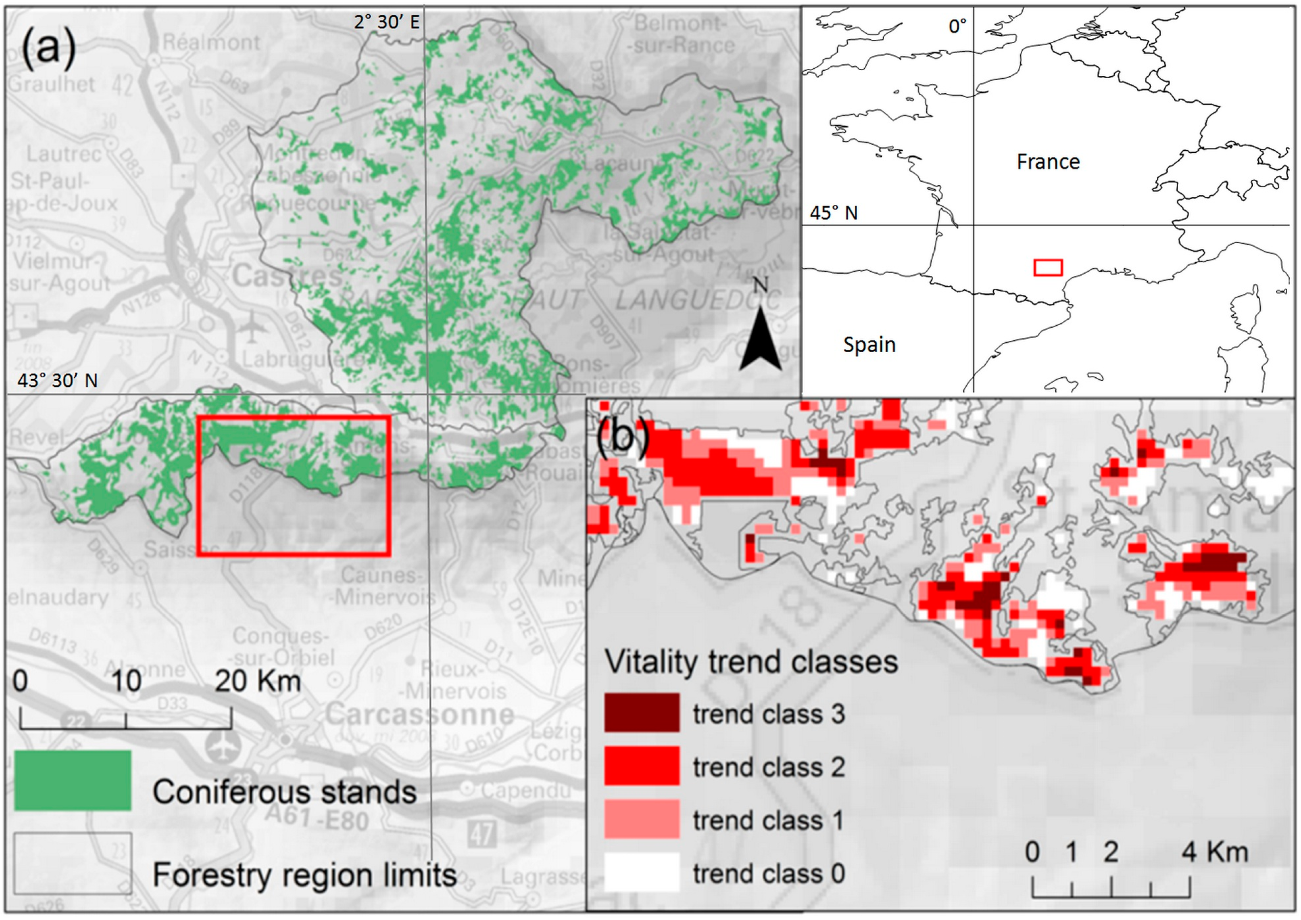
Figure 1. (a) Coniferous stands in the study area. The black triangle (∆) localize the weather station of Lacaune; (b) Excerpt from the vitality trend map; (c) Study area.

2.2. MODIS Data

In this study, we used MODIS Terra vegetation index time series produced at 250 × 250 m resolution and 16-day compositing periods (MOD13Q1 collection 5 product). These images were generated using the constrained view maximum value compositing method to limit the effects of residual clouds and atmospheric effects, and to constrain the angles [34]. Time series of 253 images acquired from February 2000 to February 2011 were obtained from the Land Processes Distributed Active Archive Center (https://lpaac.usgs.gov/). Dataset pre-processing included clipping the images to fit the study area, re-projecting the images onto the French geodesic system and correcting data errors using the adaptive Savitzky-Golay algorithm with TIMESAT Software [35]. The Savitzky-Golay filter fits a quadratic polynomial for each date to the dates included in a moving window. Here the processing window takes into account five synthesis before and after the processed date. MODIS NDVI values, theoretically coded from −1.0 to +1.0, were resampled between 0 and 255 (one byte) in order to facilitate computer processing and data storage [36]. For our analysis, only pixels located within the boundaries of forest stands were selected, i.e., 2851 MODIS pixels, covering about 17,800 hectares.

3. Methods

3.1. Map of Vitality Trends

Hereafter, the method previously developed to map forest decline is presented [12,14]. The map of vitality trends will be combined with the clear-cut detection results presented in this paper.

Using MODIS NDVI time series (2000–2010) and a phenological approach, forest stand vitality trends were mapped for the study area. Vitality trends were calculated using the Spring Greenness phenological metric (SG), which expresses the annual level of vegetation activity during the growth period [12,13,37]. The SG indicator corresponds to the sum of NDVI calculated over a fixed period of five syntheses from the onset of spring greenness (beginning of April) to the maximum NDVI (in June) before the dry season. A series of eleven SG values (one per year) was generated per pixel. A linear regression of these annual SG values was fitted using a least square approach for each pixel (Equation (1)).

$$S{G}_{ij}=\left(a_i\times Y_j\right)+b_i$$

(1)

where $a_i$ is the slope of the trend for a given pixel, $Y_j$ is the year, $b_i$ is the intercept term

The linear trend of SG values provides information on overall changes in forest stand vitality. Then, the statistical significance of the of the spring greenness trend was assessed testing the slope of the trend (a_i) against the null slope (a₀) using a Student test calculated as in Equation (2) [31].

$$t_i=\left(a_i-a_0\right)/\left({\text{σ}}_i/\sqrt{n-2}\right)$$

(2)

where $a_i$ is the slope of the trend for a given pixel, $a_0$ is the slope of the reference trend (here equal to zero), $n$ is the number of years, ${\text{σ}}_{\text{i}}$ is the standard deviation

Using the test results, the trends of SG indicator values were grouped in four classes [13,38], one class for healthy vegetation and three classes of declining vegetation:

-

Trend class 0: positive trends or trends not significantly different from the null slope, p-value > 0.05

-

Trend class 1: trends significantly negative, 0.05 > p-value > 0.01

-

Trend class 2: trends significantly negative, 0.01 > p-value > 0.001

-

Trend class 3: trends significantly negative, 0.001 > p-value

An excerpt from the trend map of the study area is presented in Figure 1b. The combination of these vitality trend classes and the clear-cut probability levels is the main goal of this work, allowing clear-cuts to be distinguished from declining stands.

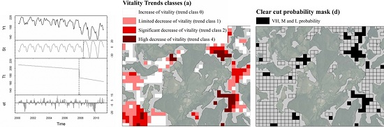
3.2. Breakpoint Detection

BFAST (Break For Additive Seasonal and Trend) uses an additive decomposition model that iteratively fits a piecewise linear trend and seasonal model [5]. The general model is of the form Yt =Tt +St +et, t = 1... n, where Yt is the observed data at time t, Tt is the trend component, St is the seasonal component, and et is the remainder component. The remainder component is the remaining variation in the data beyond that in the seasonal and trend components [39]. The trend component is modelled by a simple piecewise linear model (i.e., intercept and slope) and the seasonal component by a seasonal dummy variable [5,40].

The three components can be related to variations of activity on different time scales: (1) a “seasonal” component related to annual variations of activity i.e., phenology; (2) a “trend” component related to long term changes; and (3) a “remainder” component related to irregular short-term variations or noise (e.g., clouds or atmospheric scatter). Besides that, BFAST makes it possible to detect breakpoints in the “seasonal” and “trend” components, corresponding respectively to phenological changes and to abrupt changes (e.g., clear-cuts). The “break” parameter (maximum number of detected breakpoints) was set to 1 in order to detect only one major breakpoint during the 2000–2010 period. The “h” parameter (fraction of the entire time series between potential breakpoints) was set to 0.1, indicating approximately one year between two potential breakpoints. The presence of a breakpoint was estimated by the ordinary least squares residuals-based moving sum test (MOSUM), p-value = 0.05. For each of the 2851 pixels in the study area, the date and magnitude of the detected breakpoint were extracted. A positive breakpoint magnitude value means an abrupt increase in activity, while a negative magnitude value means an abrupt decrease in activity, possibly due to clear-cutting.

Figure 2 illustrates the BFAST breakdown of an NDVI time series for 2000–2010, for a single pixel of coniferous forest, with a major breakpoint detected. These analyses were performed using the bfast package in the R statistical environment.

3.3. Clear-Cut Probability Model

Breakpoints detected using BFAST were used to implement a clear-cut detection model, based on an induced abrupt decrease in activity. Considering the heterogeneity in the size of clear-cut areas, a probabilistic approach was preferred over a conventional binary classification. The probabilistic approach used here provides additional information for quantifying the degree of uncertainty. A clear-cut reference layer has to be created for model calibration.

Figure 2. BFAST breakdown of NDVI time series for the 2000–2010 period for a single pixel of coniferous stand. Yt = original time series, St = Seasonal component, Tt = Trend component, et = Remainder component. (---): breakpoints in the seasonal and trend components.

Figure 2. BFAST breakdown of NDVI time series for the 2000–2010 period for a single pixel of coniferous stand. Yt = original time series, St = Seasonal component, Tt = Trend component, et = Remainder component. (---): breakpoints in the seasonal and trend components.

3.3.1. Clear-Cut Reference Layer

In the first step, clear-cuts in the study area were digitized by interpreting aerial photographs acquired by the French National Geographic Institute (IGN) in 2003 and 2010. (IGN Website: www.geoportail.gouv.fr). In the study area, 28% of MODIS pixels within the forest stand boundaries were characterized by the presence of a clear-cut. Analysis of the digitized clear-cut areas revealed major differences in size (mean area = 2.80 ha, standard deviation = 4.63 ha) with a high proportion of very small patches. Consequently, only a few pixels on the MODIS grid were characterized by a large clear-cut area. Actually, only five pixels are fully covered by a clear-cut, which is not sufficient for calibrating the clear-cut detection model.

In the second step, we needed to allocate the presence or the absence of clear-cutting to a pixel and thereby set up binary reference data to be used for calibration. It was therefore necessary to define a threshold for the proportion of clear-cuts in a pixel area. This threshold had to fulfill two requirements: (1) a sufficient number of pixels considered as cut and (2) a clear-cut surface within the pixel large enough to significantly alter the signal and be detected as a sudden change of activity. These characteristics vary in the opposite direction. It was therefore necessary to define an intra-pixel clear-cut proportion threshold to address these two requirements.

The thresholding method used here is based on establishing Receiver Operating Characteristic (ROC) curves. The ROC curve is a graph showing the true positive rate (sensitivity) versus the false positive rate (1—specificity) over a range of threshold values [41]. ROC curves are increasingly used to analyze change using satellite images [42]. The principle of the ROC curve is to analyze the relationship between a continuous variable and a binary variable. Here, the continuous variable is the slope coefficients of the trends of SG. The binary variable will be the clear-cut reference data, with two modalities: “clear-cut” and “no clear-cut”. This relationship was established for 10 situations, each corresponding to a threshold proportion of clear-cut area in the pixel, going from 10% to 100%, in 10% increments. MODIS pixels were classified according to “presence of clear-cut” if the intra-pixel proportion of clear-cut was above the threshold, and “absence of clear-cut” if the intra-pixel proportion of clear-cut was below the threshold. ROC curve analyses were conducted using the ROCR package [43] in R the statistical environment (http://cran.r-project.org/).

Using the 10 proposed thresholds, 10 ROC curves were generated, for each one the strength of the relationship between the two variables was quantified by calculating the area under the ROC curve (AUC) statistic. These clear-cut reference layers defined by the different thresholds of intra-pixel proportion of clear-cut area were used for model calibration.

3.3.2. Calibration of the Clear-Cut Probability Model

The aim was to establish breakpoint magnitude thresholds in order to dissociate significantly different populations of pixels depending on the presence or absence of clear-cut. First, the relationship between the probability of the presence of clear-cut and the magnitude of the breakpoint values was observed. Then, we used a recursive partitioning technique known as a “conditional inference tree” [44] to establish probability classes for the presence of clear-cut, using the magnitude values of the detected breakpoints as a continuous predictive variable. A conditional inference tree is a non-parametric method that splits a dataset into two populations based on the association between one or more continuous predictors and a target variable, in order to build a decision tree. The main advantages of decision trees over logistic regression methods are that they make it possible to study interactions between non-parametric variables and highlight interactions, such as threshold effects, that are difficult to identify with regression logistic methods. Moreover, one of the advantages of the conditional inference tree used here is the existence of a statistical criterion linked to tree node establishment in order to separate two sub-populations, thus providing the strongest possible separability threshold. Tree growth is based on statistical stopping rules, so pruning should not be required. The decision tree is set up with a population separation criterion of 2 (at least two distinct populations are used to estimate the presence of a node) and Monte Carlo tests (p-value = 0.05; 9999 replications) to estimate the significance of the nodes. In order to limit the complexity of the model, the number of successive nodes is limited to three, maintaining a limited number of sub-populations.

To implement the clear-cut probability model, we selected pixels characterized by the detection of a breakpoint between 2003 and 2010, to be consistent with the acquisition dates of the aerial photographs used to digitize the clear-cut reference data (1601 pixels out of the 2851 pixels in the study area). To calibrate the decision tree-based model, we randomly sampled 50% of the selected pixels (833 pixels). The remaining pixels were used to assess the accuracy of the model. Analyses were conducted using the ctree function from the party package in the R statistical environment.

3.3.3. Assessment of the Accuracy of the Clear-Cut Detection Model

This approach was developed earlier to assess the accuracy of clear-cut detection derived from MODIS imagery in boreal forest [17]. The three thresholds identified by the model were used to create three binary layers from the breakpoint magnitude layer classified as “clear-cut” and “no clear-cut”. Using the pixels previously set aside to validate the model (768 pixels), the clear-cut reference data (proportion of intra-pixel clear-cut area greater than 30%) was compared to each of the three binary layers to process confusion matrices [45]. Confusion matrices were used to calculate errors of omission (Equation (3)) and commission (Equation (4)).

$$\text{Errors of omission}=\frac{\text{pixels of clear - cut in the reference but not identified as clear - cut by the model}}{\text{pixels of clear - cut in the reference}}$$

(3)

$$\text{Errors of commission}=\frac{\text{pixels of no clear - cut in the reference but identified as clear - cut by the model}}{\text{pixels identified as clear - cut by the model}}$$

(4)

Errors of commission correspond to clear-cut detected by the model although not validated by the reference data. Errors of omission point to clear-cuts identified in the reference data but not by the model. Finally, the mean and standard deviation of the errors of omission and commission were calculated in order to evaluate the accuracy of the model.

3.3.4. Effect of the Intra-Pixel Clear-Cut Proportion on the Accuracy of Clear-Cut Detection

To estimate the effect of the intra-pixel clear-cut area on the model’s accuracy, errors of omission and commission were estimated for each reference layer calculated with the different proportions of intra-pixel clear-cut (10%, 20%, 30%, 40%, 50%, 60%, 70%, 80%, 90% and 100%) [17]. The two errors were estimated for each of the three model-derived thresholds, using all the study area pixels.

4. Results

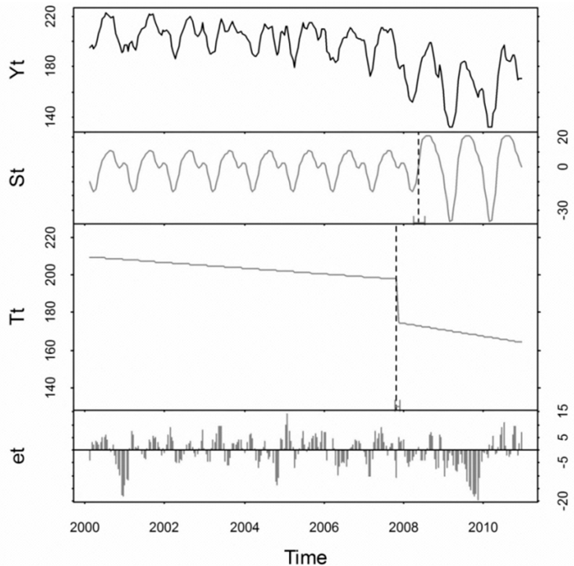
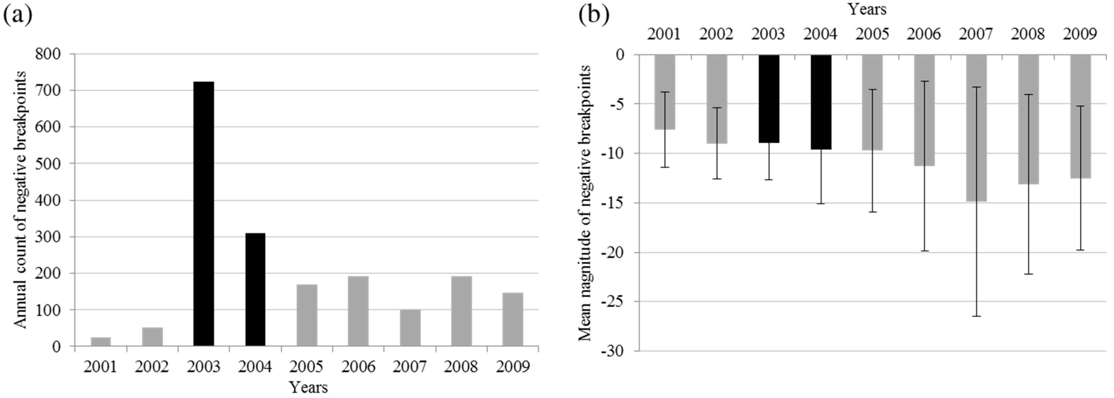
4.1. Dates and Magnitudes of Detected Breakpoints

Using BFAST, a major breakpoint was detected for each of the 2851 pixels between 2001 and 2009. By setting the “h” parameter to 0.1, we restrict breakpoint detection to periods longer than one year. No breakpoint was detected in the first and last years of the series, 2000 and 2010. The results showed that 93% of pixels were characterized by at least one breakpoint in the “trend” component, whether positive or negative. Altogether, there were 29% positive breakpoints and 71% negative breakpoints.

Only negative breakpoints were selected; they represent an abrupt decrease in activity due to a severe decline in stand vitality or clear-cutting. Annual breakpoint count and their magnitudes were analyzed. Figure 3 shows the annual count and the mean magnitude of the negative breakpoints over the 9 years of the study period.

Breakpoint counts revealed significant temporal variability. Indeed, most negative breakpoints were identified during the years 2003 and 2004. Prior to 2003–2004 the breakpoint count was very low, and after that the annual count was relatively high (Figure 3a). There was also a high intra-annual variation between the magnitude values (Figure 3b); magnitude standard deviation increased significantly after 2004, and was particularly high in 2007. These observations led to the identification of three periods and can be illustrated by rainfall data (Table 1) measured at Lacaune weather station (Figure 1a):

-

The 2001–2002 period was characterized by a low negative breakpoint count, low magnitudes and limited standard deviations. No major climate anomalies or unscheduled clear-cutting activity was identified during this period.

-

The 2003–2004 period was characterized by a high negative breakpoint count with low magnitudes. This may be related to the direct impact of the 2003 summer drought and heat wave on the vitality of the forest stands [46]. After 2003, some stands were affected by pathogen attacks or by intense drying [47]. Furthermore, the low accumulation of reserves during the summer of 2003 led to a lack of activity during 2004 spring [48].

-

The 2005–2009 period was characterized by a medium negative breakpoint count with high magnitudes and standard deviations. Many clear-cuts were made further to the significant degradation of some stands after the 2003 summer drought. The summers of 2005 and 2006 were also characterized by a severe drought that may have impacted some forest stands. All the clear-cuts during this period can be associated with decaying stands presenting a high tree mortality rate.

Figure 3. (a) Annual count of negative breakpoints; (b) The mean magnitude of negative breakpoints; whiskers represent +/− one standard deviation.

Figure 3. (a) Annual count of negative breakpoints; (b) The mean magnitude of negative breakpoints; whiskers represent +/− one standard deviation.

Table 1. Rainfall data from Lacaune weather station: annual and summer rainfall (mm) for the studied years (2000 to 2010) and 30 years average (1981 to 2010).

Period	2000	2001	2002	2003	2004	2005	2006	2007	2008	2009	2010	1981–2010
Annual	1459	1153	1471	1240	1499	1048	1199	1298	1486	1277	1216	1409
June, July, August	580	459	614	199	539	283	338	491	481	450	362	461

Table 1. Rainfall data from Lacaune weather station: annual and summer rainfall (mm) for the studied years (2000 to 2010) and 30 years average (1981 to 2010).

Period	2000	2001	2002	2003	2004	2005	2006	2007	2008	2009	2010	1981–2010
Annual	1459	1153	1471	1240	1499	1048	1199	1298	1486	1277	1216	1409
June, July, August	580	459	614	199	539	283	338	491	481	450	362	461

4.2. Clear-Cut Probability Model

4.2.1. Clear-Cut Reference Layers

Figure 4 shows the area under the ROC curve (AUC) statistic calculated for each of the 10 threshold values of the proportion of intra-pixel clear-cut area. AUC values rose as a function of the proportion of the intra-pixel clear-cut area. AUC statistics range from 0.5 for the absence of any relationship between variables to 1 in the context of a perfect relationship. We conclude that the higher the proportion of intra-pixel clear-cut area, the stronger the relationship with vitality trend values (i.e., >30% clear-cut threshold).

Concurrently, for each threshold proportion of clear-cut area in a pixel, from 10% to 100%, the percentage of pixels for the “clear-cut” modality in the study area was calculated. The “percentage of clear-cut pixels” curve (Figure 4) decreases from 17.6%, when the intra-pixel clear-cut area is equal to 10% or lower, to 0.2%, when the intra-pixel clear-cut area is equal to 100%.

Figure 4. AUC values and percentage of “cut” pixels in the study area, as a function of the proportion of intra-pixel clear-cut.

Figure 4. AUC values and percentage of “cut” pixels in the study area, as a function of the proportion of intra-pixel clear-cut.

We can thus observe an increase in the AUC statistic with the increase in the proportion of the intra-pixel clear-cut area, while the percentage of clear-cut pixels decreases. The intersection point between the two graphs defines the optimal values for the two statistics. The threshold of intra-pixel clear-cut used for the development of clear-cut reference data will be 30%. It corresponds to an acceptable AUC statistic (AUC > 0.9) and an adequate proportion of “cut” pixels to calibrate the model (9.1%).

Finally, a binary clear-cut reference layer was derived at MODIS NDVI image resolution (250 m), with two modalities: “cut” if at least 30% of the pixel area was clear-cut during the study period and “uncut” if less than 30% of the pixel area was clear-cut during the study period.

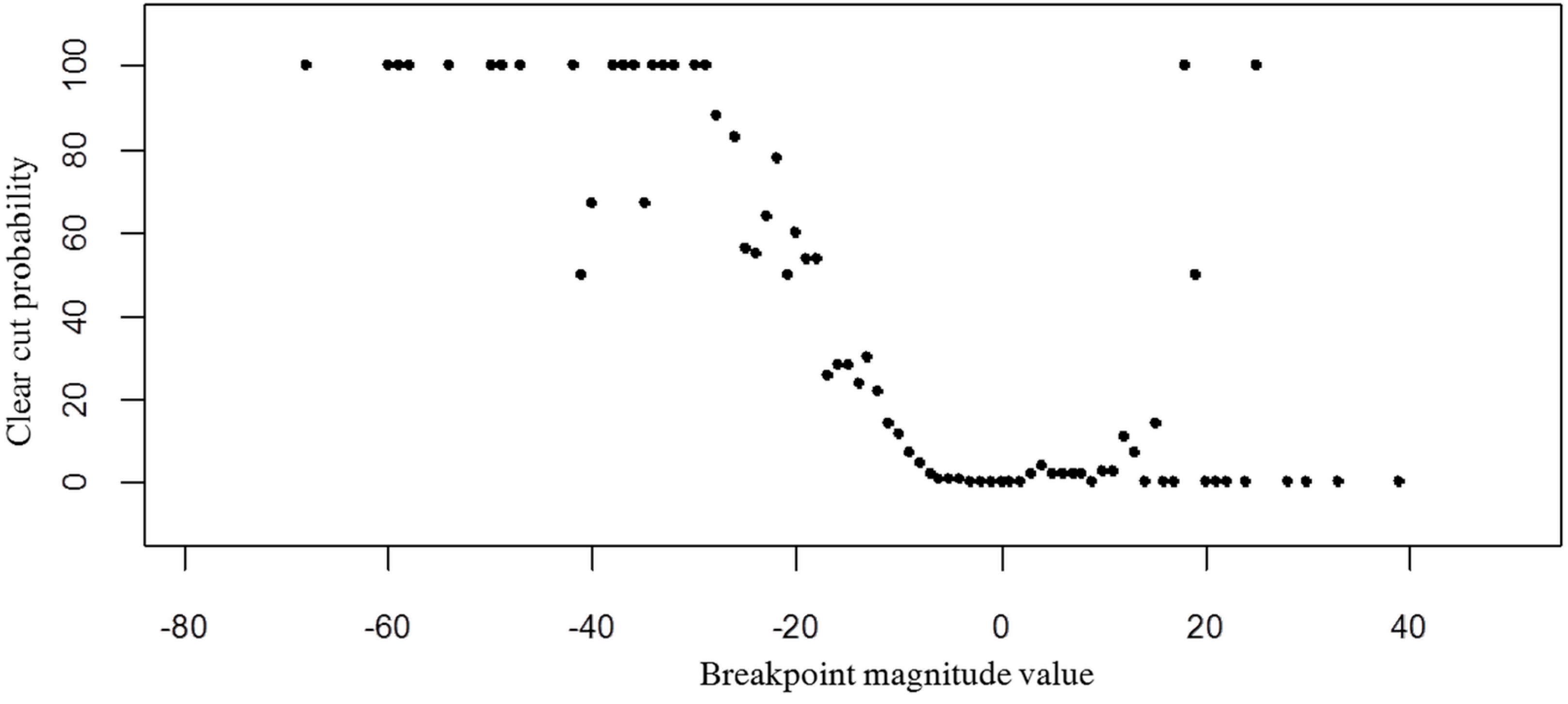
4.2.2. Relationship between Clear-Cut Probability and Breakpoint Magnitude

Figure 5 shows the clear-cut probability according to breakpoint positive or negative magnitude values. Three different situations can be seen: (1) probabilities close to 100% and high negative magnitude values, from −70 to −30; (2) a quasi-linear relationship between clear-cut probabilities and breakpoint magnitudes when these values range from −30 to −10 and (3) probabilities equal or close to 0% and low negative or positive magnitude values, from −10 to 40. This nonlinear relationship between clear-cut probability and breakpoint magnitude values demonstrates the need to determine the magnitude thresholds, in order to define clear-cut probability classes.

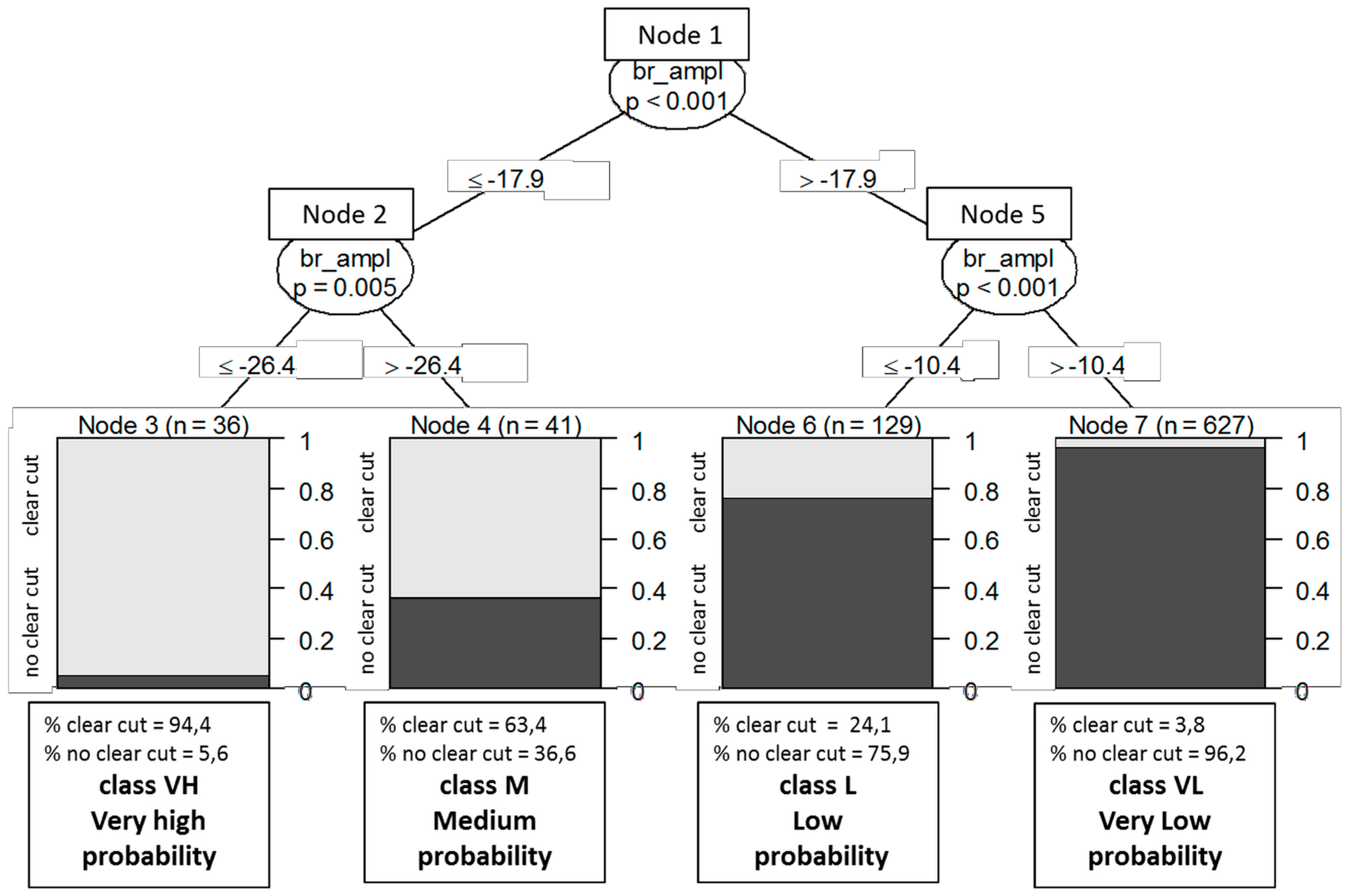
4.2.3. Definition of Clear-Cut Probability Classes

A conditional inference tree was generated to estimate the probability of clear-cut. The detected breakpoints’ magnitude values were used as input variables. All magnitude values were used, not just negative values. The target variable corresponds to the two modalities “clear-cut” and “no clear-cut” from the reference layer (see Section 4.2.4). The result is shown in Figure 6.

Figure 5. Relationship between clear-cut probability and breakpoint magnitude.

Figure 5. Relationship between clear-cut probability and breakpoint magnitude.

Figure 6. Conditional inference tree for predicting the presence of clear-cuts (at least 30% of the pixel area). Input variable: magnitude of the breakpoint (br_ampl) detected during the 2001–2009 period. Target variable with 2 modalities: clear-cut and no clear-cut (cut and nocut). The light gray bars at the terminal nodes represent the empirical probability of clear-cuts. Monte Carlo permutation test, p-value = 0.05, Max Depth = 3.

Figure 6. Conditional inference tree for predicting the presence of clear-cuts (at least 30% of the pixel area). Input variable: magnitude of the breakpoint (br_ampl) detected during the 2001–2009 period. Target variable with 2 modalities: clear-cut and no clear-cut (cut and nocut). The light gray bars at the terminal nodes represent the empirical probability of clear-cuts. Monte Carlo permutation test, p-value = 0.05, Max Depth = 3.

The conditional inference tree output consisted of four classes of pixels characterized by their proportion of “cut” or “no cut” pixels. The light gray bars at the terminal nodes represent the empirical probability of clear-cuts. The clear-cut probability values ranged from 4% (rightmost bar chart) to 94% (leftmost bar chart). Three magnitude thresholds were identified: −26.4, −17.9 and −10.4 to establish these four classes.

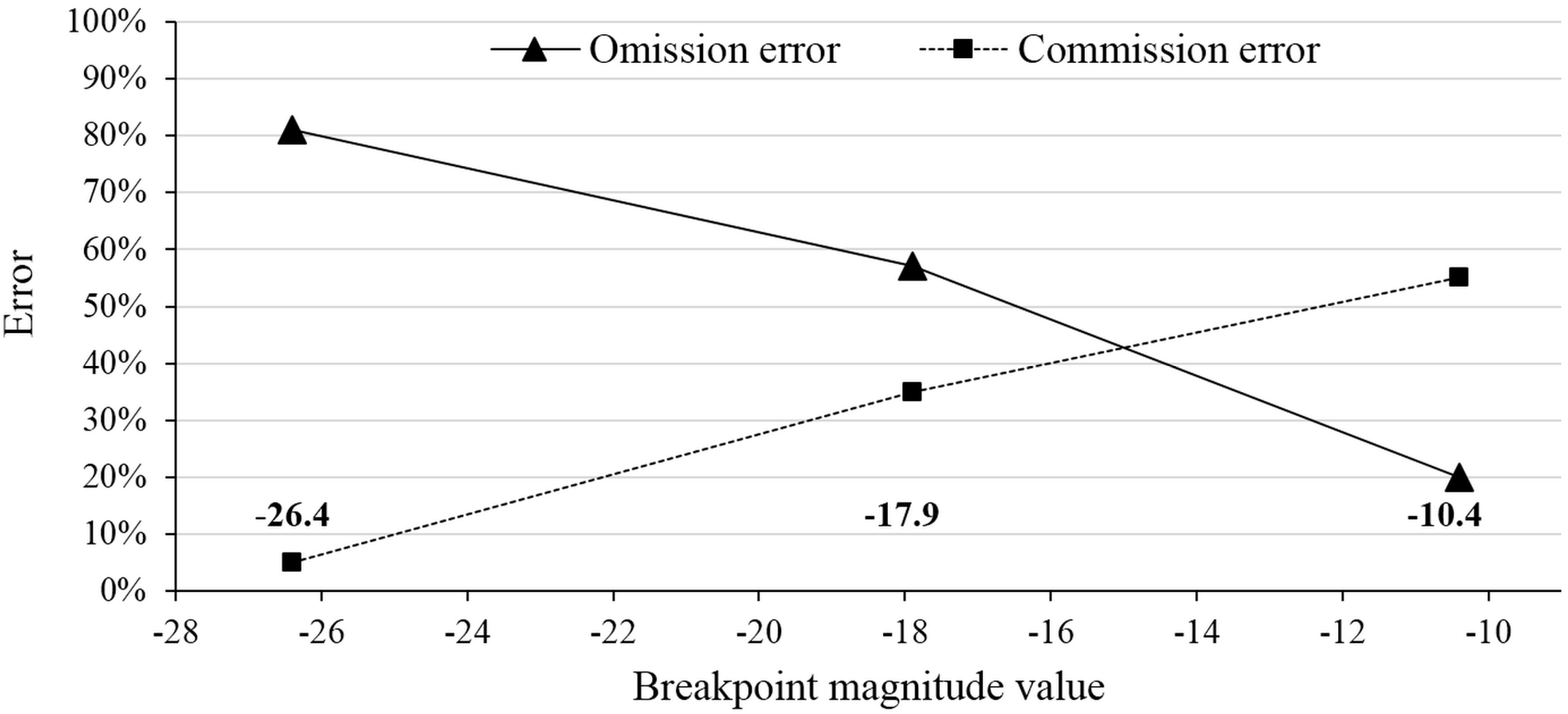
4.2.4. Accuracy of the Clear-Cut Detection Model

To transform probability values into binary projections for each of the three thresholds, the pixels were successively classified as “cut” if the magnitude value was below the threshold concerned and as “no cut” if the breakpoint magnitude value was above the threshold.

The evolution of the errors of omission and commission, from strongly negative to low negative close to about zero breakpoint magnitudes, was established in Figure 7 for each threshold value: −26.4, −17.9 and −10.4.

Figure 7. Errors of commission and omission trends according to the model’s thresholds.

Figure 7. Errors of commission and omission trends according to the model’s thresholds.

At the −26.4 threshold, the error of commission was very low close to zero (5%), but the error of omission was high (81%). Then, at the intermediate threshold (−17.9), the error of omission (57%) was still higher than the error of commission (35%). The error of commission (55%) only exceeded the error of omission (20%) for the last threshold value (−10.4). The shift in the errors of omission and commission between the two extreme threshold values illustrates the importance of threshold selection in the context of a specific application.

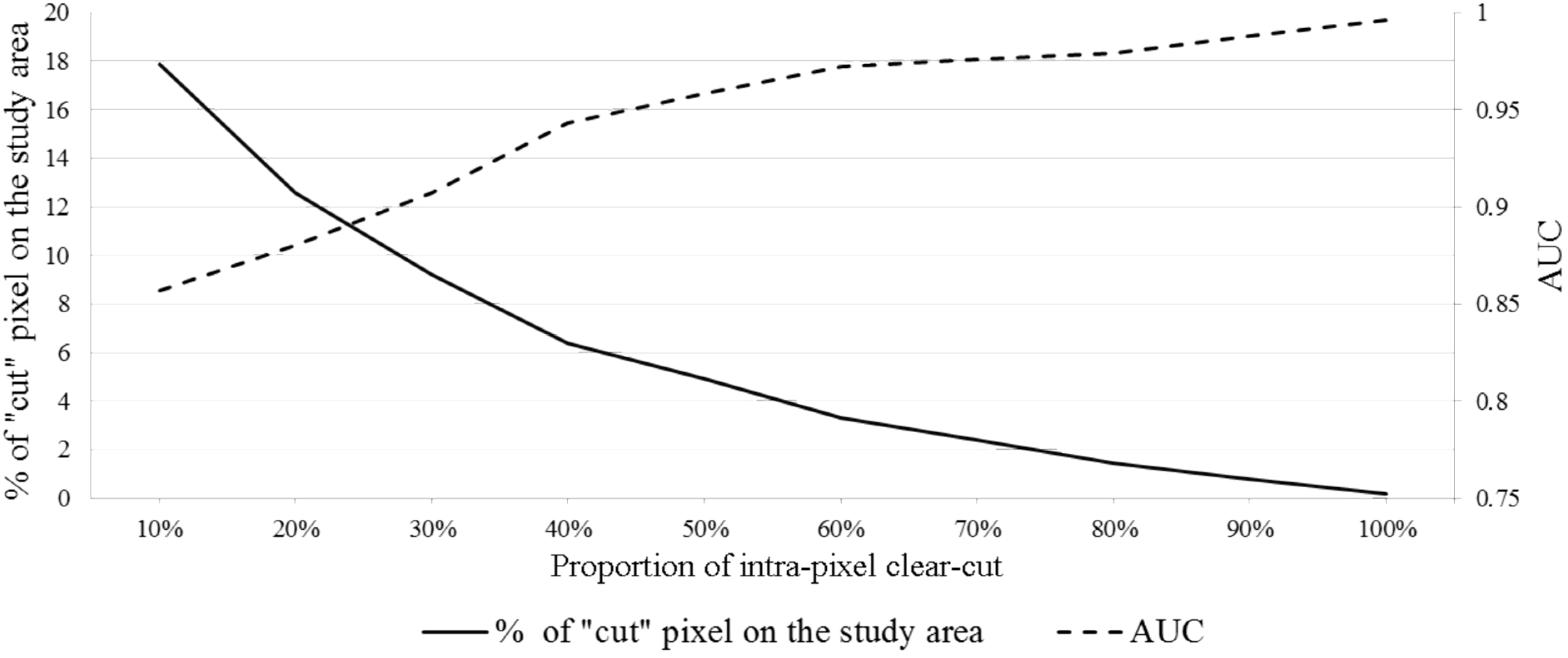
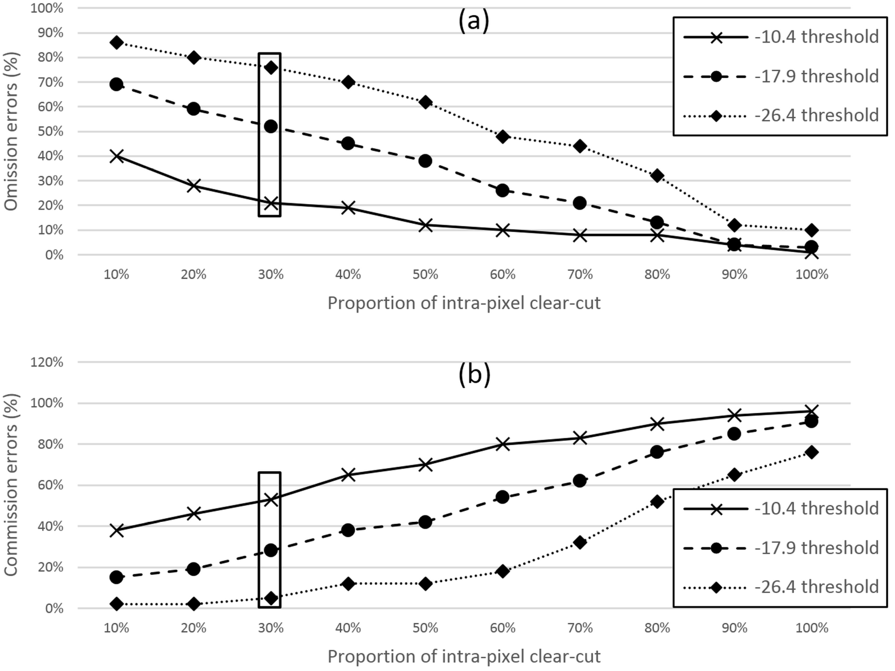
4.2.5. Impact of the Intra-Pixel Clear-Cut Proportion on the Accuracy of Clear-Cut Detection

Figure 8 shows errors of omission and commission according to the proportion of intra-pixel clear-cuts in the reference data for the three thresholds derived from the clear-cut detection model. Overall, the errors of omission decreased with an increase in the intra-pixel proportion of clear-cut (Figure 8a). Conversely, errors of commission increased with an increase in the percentage of intra-pixel clear-cuts (Figure 8b). For example, taking pixels with at least 90% of clear-cuts as reference and the threshold value of −10.4 errors of omission were low (4%), but the error of commission was high (94%). Conversely, taking pixels with at least 10% of clear-cut as reference, the error of omission was higher (40%) and the error of commission was lower (38%). We can confirm that selecting pixels with a very low clear-cut area significantly increased errors of omission, and therefore the inaccuracy of the model. Conversely, only selecting pixels with a high proportion of intra-pixel clear-cut greatly increased the errors of commission. In this case, more pixels with a small proportion of pixels were excluded from the clear-cut reference data, even if they were detected by the model. The threshold of 30% of intra-pixel clear-cut used to calibrate the model enabled a good trade-off between errors of omission and errors of commission, respectively 21% and 53% for the −10.4 threshold.

Figure 8. (a) Errors of omission and (b) Errors of commission according to the proportion of intra-pixel clear-cut in the reference clear-cut data, for each model-derived threshold.

Figure 8. (a) Errors of omission and (b) Errors of commission according to the proportion of intra-pixel clear-cut in the reference clear-cut data, for each model-derived threshold.

4.3. Characterization of Clear-Cut Probability Classes

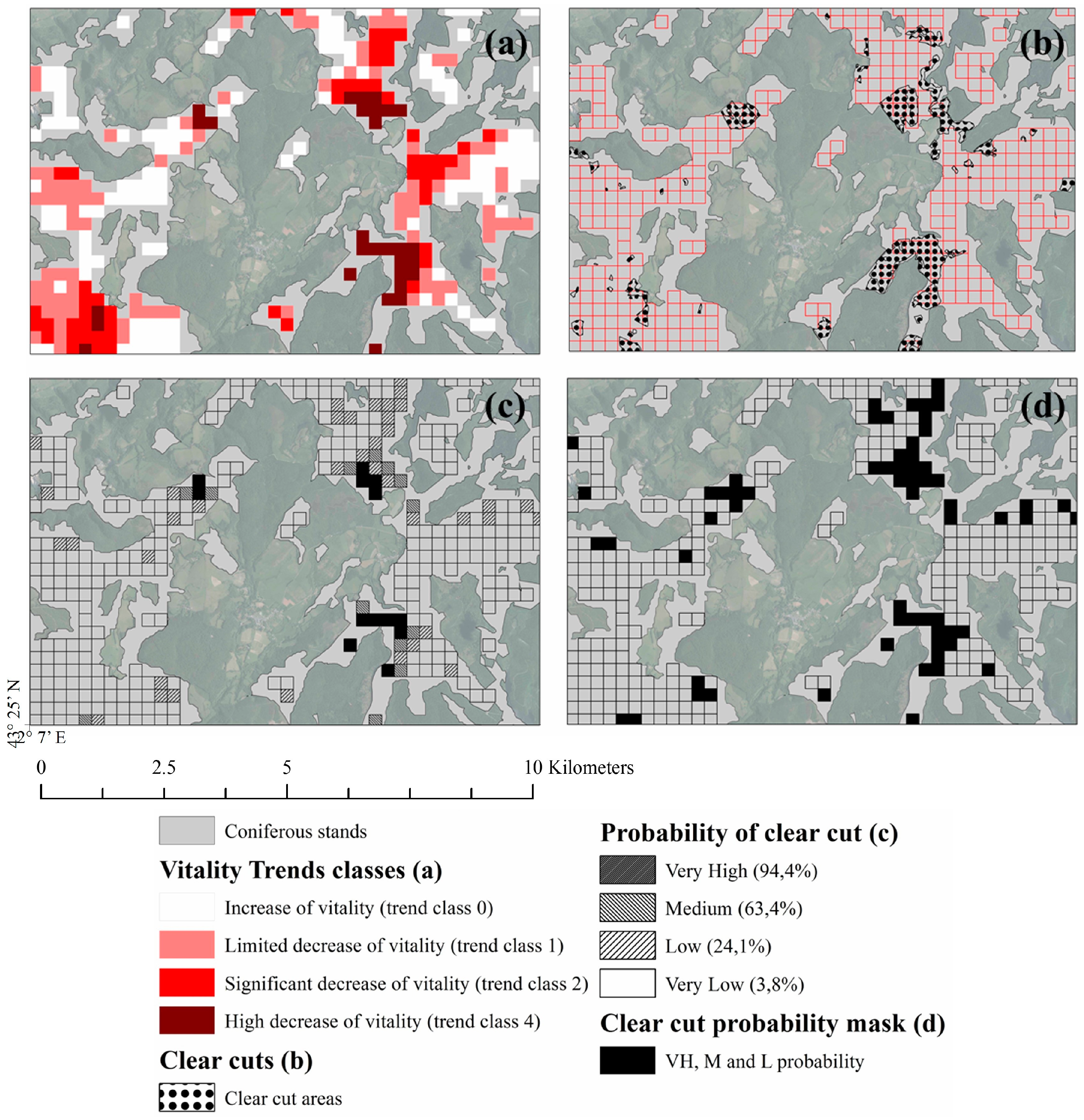
4.3.1. Spatial Distribution of Clear-Cut Probability Classes

Table 2 lists the four previously defined classes of clear-cut probability. Class M and class L correspond to a highly uncertain estimation of the presence or absence of clear-cut (24% probability for class L and 63% for class M). The pixels in these two classes cover 2705 ha (18% of the study area). Classes VL and VH correspond to situations with a few errors in the estimation of the presence or absence of clear-cut. Class VL, corresponding to 96% probability of no clear-cut, covers 12,262 ha (80% of all pixels). Class VH, which corresponds to 94% probability of clear-cuts, covers 333 ha (2% of all pixels).

The average proportion of intra-pixel clear-cut area was calculated for each class (Table 2). Results showed statistically significant differences between all classes (Kruskal-Wallis test, p-value = 0.05). The average proportion of intra-pixel clear-cut area ranged from 3.8% for class VL to 69.2% for class VH. This confirms the fact that probability classes are closely related to the proportion of intra-pixel clear-cut area. The greater the increase in the intra-pixel clear-cut area, the higher the probability of clear-cut. On the other hand, below 16.7% of intra-pixel clear-cut (less than 1 ha), there is a lower probability of clear-cut.

Out of the 15,300 ha of the study area, 1100 ha of clear-cuts were identified by interpreting aerial photographs. From the model, and when class M and class VH were combined, the estimated clear-cut area was 918 ha, i.e., an underestimation of 182 ha (16.5% of the clear-cut area). When three classes, L, M and VH, were combined, the estimated clear-cut area was 3038 ha, i.e., a major overestimation of 1938 ha (176% of the clear-cut area).

Table 2. Summary of characteristics of clear-cut probability.

Clear-Cut Probability Classes	Breakpoint Magnitude Threshold	Clear-Cut Presence Probability	Proportion of Pixel in the Study Area (Total Area)	Intra-Pixel Clear-Cut Proportion in a MODIS Pixel
		%	% (ha)	Mean and (standard deviation) %
VL – Very low probability of clear-cut	−10.5; +∞	3.8	80.1% (12 262 ha)	3.8% (9.8)
L – Low probability of clear-cut	−17.9; −10.5	24.1	13.8% (2 120 ha)	16.7% (20.1)
M – Medium probability of clear-cut	−26.4; −17.9	63.4	3.8% (585 ha)	35.1% (24.8)
VH – Very high probability of clear-cut	− ∞; −26.4	94.4	2.7% (333 ha)	69.2% (22.9)

Table 2. Summary of characteristics of clear-cut probability.

Clear-Cut Probability Classes	Breakpoint Magnitude Threshold	Clear-Cut Presence Probability	Proportion of Pixel in the Study Area (Total Area)	Intra-Pixel Clear-Cut Proportion in a MODIS Pixel
		%	% (ha)	Mean and (standard deviation) %
VL – Very low probability of clear-cut	−10.5; +∞	3.8	80.1% (12 262 ha)	3.8% (9.8)
L – Low probability of clear-cut	−17.9; −10.5	24.1	13.8% (2 120 ha)	16.7% (20.1)
M – Medium probability of clear-cut	−26.4; −17.9	63.4	3.8% (585 ha)	35.1% (24.8)
VH – Very high probability of clear-cut	− ∞; −26.4	94.4	2.7% (333 ha)	69.2% (22.9)

4.3.2. Annual Distribution of Clear-Cut Probability Classes

The annual distribution of breakpoints was expressed as a percentage of the total detected breakpoints for the 2001–2009 period. Figure 9 shows the temporal evolution of the detected breakpoints for the combination of very low and low clear-cut probabilities (classes VL and L) (Figure 9a) and medium plus very high probabilities (classes M and VH) (Figure 9b).

Figure 9. Annual distribution of (a) Low and Very-Low clear-cut probability (% of all classes) and (b) Medium and Very High clear-cut probability (% of all classes).

Figure 9. Annual distribution of (a) Low and Very-Low clear-cut probability (% of all classes) and (b) Medium and Very High clear-cut probability (% of all classes).

Breakpoints with low and very low clear-cut probabilities occurred mainly in 2003 and 2004. These high proportions (respectively 24% and 13%) must be related to the large number of breakpoints detected in these two consecutive years. They reflect the abrupt decrease in stand vitality that occurred during and just after the 2003 summer drought. Breakpoints with medium and very high clear-cut probabilities (classes M and VH) increased from 2003 and became higher from 2006, especially in 2008. During this period, numerous clear-cuts, sometimes covering large areas, were made.

4.3.3. Relationship between Clear-Cut Probability Classes and Stand Vitality Trend Classes

The four classes defined using the slope coefficients of SG trends can be interpreted to describe stand vitality:

-

Trend class 0: Increase or no significant decrease in vegetation activity, probably healthy stands;

-

Trend class 1: Limited decrease in vegetation activity, stand development uncertain;

-

Trend class 2: Significant decrease in vegetation activity, most forest stands are declining;

-

Trend class 3: Very high decrease in vegetation activity, declining stands, usually cut down.

Figure 10 shows extracts from the map of the study site illustrating our results. The vitality trends (Figure 10a) can be compared with the clear-cuts map (Figure 10b) so we can observe that while clear-cuts often dominate trend class 3, it is actually impossible to distinguish them from pixels in which forest vitality is seriously declining.

Clear-cut probability and stand vitality trend were overlaid. Figure 11 shows the distribution of clear-cut probability classes for each vitality trend class. In trend class 3, which corresponds to a considerable decrease in the vitality of the stands, there was a high proportion (57%) of medium and very high clear-cut probabilities (classes M and VH). The fact that pixels affected by clear-cuts in these classes would be taken into account was already known. Otherwise, the remaining 43% (marked *1 in Figure 11) correspond to pixels characterized by a major decrease in vitality but with a very low or low probability of clear-cut. It is highly probable that these pixels correspond to a gradual decrease in vitality related to forest decline. We came to the same conclusion concerning Trend class 2 where 92% of the pixels showed a decrease in vitality probably related to forest decline (marked *2 in Figure 11). This trend class is one of the most interesting when monitoring the condition of forest stands, as it presents evidence of a decrease in vitality with a low probability of human intervention. There was no significant decrease in vitality in Trend class 0 and Trend class 1, and they contained very few pixels affected by a clear-cut.

A large area of coniferous stands is characterized by a marked decrease in vitality (Trend class 2 and Trend class 3) (Figure 10a) and several clear-cuts were made during the 2003–2010 period (Figure 10b). A clear-cut probability mask was established (Figure 10d), to focus on any decrease in forest vitality it includes low, medium and very high clear-cut probabilities (Figure 10c). This mask allowed us to distinguish stands where vitality is decreasing from clear-cut stands.

Figure 10. Extract from (a) the vitality trend map; (b) digitized clear-cut areas; (c) probability of clear-cut classes and (d) vitality trend map with the clear-cut probability mask (Low, Medium and Very High probability of clear-cut).

Figure 10. Extract from (a) the vitality trend map; (b) digitized clear-cut areas; (c) probability of clear-cut classes and (d) vitality trend map with the clear-cut probability mask (Low, Medium and Very High probability of clear-cut).

Figure 11. Distribution of clear-cut probability classes within vitality trend classes (% of pixels per vitality trend class).

Figure 11. Distribution of clear-cut probability classes within vitality trend classes (% of pixels per vitality trend class).

5. Discussion

5.1. Regional Monitoring of Decrease in Forest Vitality

The four different probability classes identified allowed us to create a clear-cut probability mask at the same spatial resolution as a MODIS image. The interpretation and use of these four classes depended on the objectives of the analysis that we ourselves set up:

(1)

For the quantification of clear-cut areas, the medium and high clear-cut probability classes (class M and class VH) are of particular interest for users. By combining these two classes, the majority of large area clear-cuts are detected. However, the comparison with clear-cut reference data revealed an underestimation of approximately 16% of the total clear-cut area. The error of omission is mainly related to small clear-cut areas which do not generate a strong enough breakpoint to be included in class M and class VH. The majority of small clear-cut areas (less than 1 ha) are detected in class L, but this class also includes the signal for disturbances not related to clear-cuts. In this case, adding the results of this class to the clear-cut probability mask revealed a significant overestimation of about 176% of clear-cut area. For the quantification of clear-cut areas, it is preferable to limit the analysis to classes M and VH. Detecting small clear-cut areas using MODIS imagery remains out of reach [17]. We can assume that the model will be more efficient in other study areas where clear-cut areas are larger (e.g., Canada, Brazil). It may thus be necessary to assess the robustness of the method in areas with less fragmented stands and fewer stands impacted by clear-cuts.

(2)

For monitoring decreases in forest vitality, the interest of clear-cut probability classes lies in the possibility of establishing a mask that can be superimposed over a vitality trend map for the same period. By combining class L, class M and class VH to make the mask, we were able to identify, with a few errors, the location of areas impacted by clear-cuts. For the remaining pixels (class VL), the probability of the absence of clear-cuts was 96.2% (Figure 6).

We have already demonstrated that a high proportion of pixels in trend classes 2 and 3 shows a significant decrease in vitality (Figure 11) resulting from a gradual decline of health, with no major breakpoint corresponding to the pressure exerted by a clear-cut. This was also the case for trend class 1, which included some sudden disturbances. The clear-cut mask makes it possible to identify stands showing signs of forest decline that can be characterized and monitored over time (surface, degradation intensity, spatial distribution, etc.).

5.2. Methodological Considerations

The proposed probabilistic clear-cut detection model is based on a conditional inference tree estimate.

The accuracy of the model depends to a great extent on the thresholds chosen. Errors of omission ranged from 19% to 81% depending on the threshold. Conversely, errors of commission ranged from 5% to 54%. Numerous clear-cut detection studies based on analysis of MODIS images involved a high number of errors of commission. For example, in a boreal forest, using the Change Vector Analysis method, [17] reported errors of omission and commission of the same order as those observed in our study (29% and 90%, respectively). Similarly, using multiple analysis of change, [15] reported errors of omission and commission of 26% and 68%, respectively. These results confirm the potential of BFAST for detecting clear-cuts. Taking the −10.4 threshold as reference, our errors of omission and commission (19% and 54%, respectively) are of the same order as those reported in the literature. It has been shown that the accuracy of the model can be improved by removing isolated pixels classified as clear-cut [17]. However, in our study, this approach was not suitable because of the high number of isolated pixels. In these circumstances, the number of errors of commission would be lower, but many clear-cuts would ultimately not be included in the analysis and the errors of omission would not be adequate. As shown in Section 4.2.3, the intra-pixel proportion of clear-cut used to establish the reference data had a major impact on the model outputs. Tests showed that the 30% threshold represents a good trade-off between commission and omission rates. Moreover, the comparison of clear-cut periods from photointerpretation of orthophotographs (2003–2006 and 2006–2010) and the date of breakpoints on the study site (grouped into the two periods 2003–2006 and 2006–2010) shows an overall accuracy in dating events of 82%. It shows that the breakpoints’ date mainly corresponds to the actual clear-cut period.

In the context of the detection of clear-cuts, several questions remain:

(1) Which detection method should be used? [15,17] clearly showed that methods based on the analysis of spectral changes are better suited than methods based on textural changes. However, combining the methods improves the results.

(2) Which threshold should be applied? The results of probabilistic approaches clearly revealed the impact of the threshold on final accuracy. As we observed in our study, the more the threshold isolates pixels with a high probability of clear-cuts, the higher the omission rate. [16,20] pointed out that the definition of multiple detection thresholds offers end users greater flexibility for determining their goal, assuming a particular threshold. In our case, the choice of the threshold value was applied to achieve a specific objective: to eliminate situations with too high a clear-cut probability.

(3) What reference data should be used? For the detection of disturbances using coarse spatial resolution images, many authors use finer-resolution images such as Landsat [16,17] or field data [49] as reference data. The most important point is up-scaling from ground observations, or from a fine spatial resolution to coarser resolution information. In this study, two criteria (the proportion of pixels considered cut, and the impact of the proportion of intra-pixel clear-cut on vitality trends) were taken into account to establish reference data at the same resolution as MODIS images.

Finally: (4) how should the accuracy of a clear-cut detection model be evaluated? To define different thresholds, it is possible to use binary data for each threshold to calculate a confusion matrix and errors of omission and commission. These indicators of accuracy identify the proportion of error for each threshold. To validate their probabilistic model, some authors only take the threshold with the best trade-off between errors of omission and commission into account [50]. In our case, the omission and commission rates were calculated for each threshold to help select the most appropriate threshold for the end user. The utilization of general accuracy indicators, such as overall accuracy or Kappa index, does not fully inform the end user about the advantages and limitations of a given method [51]. This type of general index does not provide precise information about the type of error. This is why such indices were not used in this study.

5.3. Future Works and Perspectives

In this study, only the most significant breakpoints were taken into account. BFAST parameters could be adjusted to detect many other important breakpoints that occurred during the study period. Thus, there are opportunities for analyzing the relationships with different causes of potential disturbances (extreme climatic events, outbreaks of pathogens, fire events) and for studying gradual changes in activity between multiple breakpoints. It is also important to identify situations (location and date) indicating the recovery of vegetation activity and hence identify regrowth of forest stands after an extreme climatic event or a human-driven disturbance.

This approach could be used in other forest stands to assess the effects of climate change on forest stands. Positive features are first and foremost the high repetition rate and the free availability of MODIS-NDVI images. Theoretically, the magnitude breakpoint thresholds defined by the model should be directly applicable to other forest stands with a coniferous phenological behavior similar to the stands studied here. These classes of probability are used as part of a validation step and in the interpretation of the decrease in the vitality of silver fir (Abies Alba) stands in the Pyrenees, in the framework of the Pyrenees Climate Change Observatory (OPCC: http://www.opcc-ctp.org).

Even though the probabilistic approach presents interesting possibilities, compared to a binary approach, the spatial resolution of MODIS remains the most limiting factor. Several authors have evaluated the detection potential of Landsat time series [52,53] but given their low acquisition frequency, Landsat images are still difficult to process with time series analysis tools like BFAST. Landsat time series, even with more than one image per year, do not make it possible to study vegetation dynamics. Coarse resolution imagery, with frequent image acquisition and global or regional coverage is more useful for vegetation monitoring. Given the aim of this study, which is to distinguish sudden human driven changes from slow to medium degradation of forest health, long-term time series that make it possible to estimate intra-annual activity (e.g., time series of coarse resolution images) are indispensable.

The use of this type of time series analysis is encouraged by the upcoming launch of the Earth observation Sentinel-2 satellites, which will provide images with high spatial resolution—30 meters—with a revisit time of 5 days [54]. The limitation of the spatial resolution of MODIS images should be solved, allowing more accurate detection of small clear-cuts, but still enabling monitoring of intra-annual vegetation dynamics.

6. Conclusions

This study revealed the potential of MODIS images and BFAST for detecting clear-cuts. The clear-cut detection method was set up to implement clear-cut probability classes. The importance of the intra-pixel proportion regarding the probability of detecting clear-cuts is highlighted, considering variations in the errors of omission and commission as a function of intra-pixel clear-cut proportions. The limitation represented by the resolution of MODIS images was mitigated by the use of a probabilistic approach. Given the regular acquisition of MODIS images, a long-term operational assessment of clear-cut areas is possible.

The interest of remote sensing image time series for vegetation monitoring has been widely demonstrated [13,37,55]. Even if new sensors will improve the spatial resolution of the time series of remote sensing images, MODIS images, because of their archive, will remain an asset to observe gradual changes of vegetation activity. Improving forest vitality monitoring remains necessary. Furthermore, the proposed probabilistic approach can be considered an improvement when it helps to distinguish sudden changes, mainly human-driven, from gradual changes.

References

- Lindner, M.; Maroschek, M.; Netherer, S.; Kremer, A.; Barbati, A.; Garcia-Gonzalo, J.; Seidl, R.; Delzon, S.; Corona, P.; Kolström, M.; et al. Climate change impacts, adaptive capacity, and vulnerability of european forest ecosystems. For. Ecol. Manag. 2010, 259, 698–709. [Google Scholar] [CrossRef]
- Allen, C.D.; Macalady, A.K.; Chenchouni, H.; Bachelet, D.; McDowell, N.; Vennetier, M.; Kitzberger, T.; Rigling, A.; Breshears, D.D.; Hogg, E.H.; et al. A global overview of drought and heat-induced tree mortality reveals emerging climate change risks for forests. For. Ecol. Manag. 2010, 259, 660–684. [Google Scholar] [CrossRef]
- Van Mantgem, P.J.; Stephenson, N.L.; Byrne, J.C.; Daniels, L.D.; Franklin, J.F.; Fule, P.Z.; Harmon, M.E.; Larson, A.J.; Smith, J.M.; Taylor, A.H.; et al. Widespread increase of tree mortality rates in the western united states. Science 2009, 323, 521–524. [Google Scholar] [CrossRef]
- Bonan, G.B. Forests and climate change: Forcings, feedbacks, and the climate benefits of forests. Science 2008, 320, 1444–1449. [Google Scholar] [CrossRef] [PubMed]
- Verbesselt, J.; Hyndman, R.; Newnham, G.; Culvenor, D. Detecting trend and seasonal changes in satellite image time series. Remote Sens. Environ. 2010, 114, 106–115. [Google Scholar] [CrossRef]
- White, M.A.; de Beurs, K.M.; Didan, K.; Inouye, D.W.; Richardson, A.D.; Jensen, O.P.; O’Keefe, J.; Zhang, G.; Nemani, R.R.; van Leeuwen, W.J.D.; et al. Intercomparison, interpretation, and assessment of spring phenology in north america estimated from remote sensing for 1982–2006. Glob. Chang. Biol. 2009, 15, 2335–2359. [Google Scholar] [CrossRef]
- Verbesselt, J.; Hyndman, R.; Zeileis, A.; Culvenor, D. Phenological change detection while accounting for abrupt and gradual trends in satellite image time series. Remote Sens. Environ. 2010, 114, 2970–2980. [Google Scholar] [CrossRef]
- Holben, B.N. Characteristics of maximum-value composite image from temporal AVHRR data. Int. J. Remote Sens. 1986, 1417–1434. [Google Scholar] [CrossRef]
- Glenn, E.; Huete, A.; Nagler, P.; Nelson, S. Relationship between remotely-sensed vegetation indices, canopy attributes and plant physiological processes: What vegetation indices can and cannot tell us about the landscape. Sensors 2008, 8, 2136–2160. [Google Scholar] [CrossRef]
- Teillet, P.M.; Staenz, K.; William, D.J. Effects of spectral, spatial, and radiometric characteristics on remote sensing vegetation indices of forested regions. Remote Sens. Environ. 1997, 61, 139–149. [Google Scholar] [CrossRef]
- Hlásny, T.; Barka, I.; Sitková, Z.; Bucha, T.; Konôpka, M.; Lukáč, M. Modis-based vegetation index has sufficient sensitivity to indicate stand-level intra-seasonal climatic stress in oak and beech forests. Ann. For. Sci. 2015, 72, 109–125. [Google Scholar] [CrossRef]
- Chéret, V.; Denux, J.P.; Ortisset, J.P.; Gacherieu, C. Utilisation de séries temporelles d’images satellitales pour cartographier le dépérissement des boisements résineux du sud massif central. Rendez-Vous Tech. 2011, 31, 55–62. [Google Scholar]
- Lambert, J.; Drénou, C.; Denux, J.P.; Balent, G.; Chéret, V. Monitoring forest decline through remote sensing time series analysis. GISci. Remote Sens. 2013, 50, 437–457. [Google Scholar]
- Lambert, J. Evaluation des Baisses de Vitalité des Peuplements Forestiers à Partir de Séries Temporelles D’images Satellitaires—Application aux Résineux du sud du Massif Central et à la Sapinière Pyrénéenne. Ph.D. Thesis, Institut National Polytechnique de Toulouse, Université Toulouse III, Toulouse, France, 2014. [Google Scholar]
- Zhan, X.; Sohlberg, R.A.; Townshend, J.R.G.; DiMiceli, C.; Carroll, M.L.; Eastman, J.C.; Hansen, M.C.; DeFries, R.S. Detection of land cover changes using MODIS 250 m data. Remote Sens. Environ. 2002, 83, 336–350. [Google Scholar] [CrossRef]
- Fraser, R.H.; Abuelgasim, A.; Latifovic, R. A method for detecting large-scale forest cover change using coarse spatial resolution imagery. Remote Sens. Environ. 2005, 95, 414–427. [Google Scholar] [CrossRef]
- Bucha, T.; Stibig, H.-J. Analysis of MODIS imagery for detection of clear cuts in the boreal forest in north-west russia. Remote Sens. Environ. 2008, 112, 2416–2429. [Google Scholar] [CrossRef]
- Jin, S.; Sader, S.A. modis time-series imagery for forest disturbance detection and quantification of patch size effects. Remote Sens. Environ. 2005, 99, 462–470. [Google Scholar] [CrossRef]
- Morton, D.C.; DeFries, R.S.; Shimabukuro, Y.E.; Anderson, L.O.; Espirito-Santo, F.D.B.; Hansen, M.; Carroll, M. Rapid assessment of annual deforestation in the brazilian amazon using MODIS data. Earth Interact. 2005, 9. [Google Scholar] [CrossRef]
- Bontemps, S.; Bogaert, P.; Titeux, N.; Defourny, P. An object-based change detection method accounting for temporal dependences in time series with medium to coarse spatial resolution. Remote Sens. Environ. 2008, 112, 3181–3191. [Google Scholar] [CrossRef]
- Hansen, M.C.; DeFries, R.S.; Townshend, J.R.G.; Sohlberg, R.; Dimiceli, C.; Carroll, M. Towards an operational MODIS continuous field of percent tree cover algorithm: Examples using AVHRR and MODIS data. Remote Sens. Environ. 2002, 83, 303–319. [Google Scholar] [CrossRef]
- Desclée, B.; Bogaert, P.; Defourny, P. Forest change detection by statistical object-based method. Remote Sens. Environ. 2006, 102, 1–11. [Google Scholar] [CrossRef]
- Hansen, M.C.; Roy, D.P.; Lindquist, E.; Adusei, B.; Justice, C.O.; Altstatt, A. A method for integrating MODIS and Landsat data for systematic monitoring of forest cover and change in the Congo basin. Remote Sens. Environ. 2008, 112, 2495–2513. [Google Scholar] [CrossRef]
- Potapov, P.; Hansen, M.C.; Stehman, S.V.; Loveland, T.R.; Pittman, K. Combining MODIS and Landsat imagery to estimate and map boreal forest cover loss. Remote Sens. Environ. 2008, 112, 3708–3719. [Google Scholar] [CrossRef]
- Hilker, T.; Wulder, M.A.; Coops, N.C.; Linke, J.; McDermid, G.; Masek, J.G.; Gao, F.; White, J.C. A new data fusion model for high spatial- and temporal-resolution mapping of forest disturbance based on Landsat and MODIS. Remote Sens. Environ. 2009, 113, 1613–1627. [Google Scholar] [CrossRef]
- Lunetta, R.S.; Knight, J.F.; Ediriwickrema, J.; Lyon, J.G.; Worthy, L.D. Land-cover change detection using multi-temporal MODIS NDVI data. Remote Sens. Environ. 2006, 105, 142–154. [Google Scholar] [CrossRef]
- Vogelmann, J.E.; Xian, G.; Homer, C.; Tolk, B. Monitoring gradual ecosystem change using landsat time series analyses: Case studies in selected forest and rangeland ecosystems. Remote Sens. Environ. 2012, 122, 92–105. [Google Scholar] [CrossRef]
- Gao, F.; Masek, J.; Schwaller, M.; Hall, F. On the blending of the Landsat and MODIS surface reflectance: Predicting daily landsat surface reflectance. IEEE Trans. Geosci. Remote Sens. 2006, 44, 2207–2218. [Google Scholar] [CrossRef]
- Alcaraz-Segura, D.; Liras, E.; Tabik, S.; Paruelo, J.; Cabello, J. Evaluating the consistency of the 1982–1999 NDVI trends in the Iberian Peninsula across four time-series derived from the AVHRR sensor: LTDR, GIMMS, FASIR, and PAL-II. Sensors 2010, 10, 1291–1314. [Google Scholar] [CrossRef] [PubMed]
- De Jong, R.; de Bruin, S.; de Wit, A.; Schaepman, M.E.; Dent, D.L. Analysis of monotonic greening and browning trends from global NDVI time-series. Remote Sens. Environ. 2011, 115, 692–702. [Google Scholar] [Green Version]
- Jacquin, A.; Sheeren, D.; Lacombe, J.-P. Vegetation cover degradation assessment in Madagascar savanna based on trend analysis of MODIS NDVI time series. Int. J. Appl. Earth Obs. Geoinf. 2010, 12, S3–S10. [Google Scholar] [CrossRef]
- Tüshaus, J.; Dubovyk, O.; Khamzina, A.; Menz, G. Comparison of medium spatial resolution ENVISAT-MERIS and TERRA-MODIS time series for vegetation decline analysis: A case study in central Asia. Remote Sens. 2014, 6, 5238–5256. [Google Scholar] [CrossRef]
- De Jong, R.; Verbesselt, J.; Schaepman, M.E.; de Bruin, S. Trend changes in global greening and browning: Contribution of short-term trends to longer-term change. Glob. Chang. Biol. 2012, 18, 642–655. [Google Scholar]
- Huete, A.; Didan, K.; Miura, T.; Rodriguez, E.P.; Gao, X.; Ferriera, L.G. Overview of the radiometric and biophysical performance of the MODIS vegetation index. Remote Sens. Environ. 2002, 83, 195–213. [Google Scholar] [CrossRef]
- Jönsson, P.; Eklundh, L. Timesat—A program for analyzing time-series of satellite sensor data. Comput. Geosci. 2004, 30, 833–845. [Google Scholar] [CrossRef]
- Roderick, M.; Smith, R.; Cridland, S. The precision of the NDVI derived from AVHRR observations. Remote Sens. Environ. 1996, 56, 57–65. [Google Scholar] [CrossRef]
- Reed, B.C. Trend analysis of time series phenology of north America derived from satellite data. GISci. Remote Sens. 2006, 43, 1–15. [Google Scholar] [CrossRef]
- Lambert, J.; Jacquin, A.; Denux, J.P.; Chéret, V. Comparison of two remote sensing time series analysis methods for monitoring forest decline. In Proceedings of the 6th International Workshop on the Analysis of Multi-Temporal Remote Sensing Images (Multi-Temp), Trento, Italy, 12–14 July 2011; pp. 93–96.
- Cleveland, R.; Cleveland, W.; McRae, J.; Terpenning, I. Stl: A seasonal-trend decomposition procedure based on Loess (with discussion). J. Off. Stat. 1990, 6, 3–73. [Google Scholar]
- Makridakis, S.; Wheelwright, S.C.; Hyndman, R.J. Forecasting: Methods and Applications, 3rd ed.; John Wiley & Sons: New York, NY, USA, 1998; p. 638. [Google Scholar]
- Fawcett, T. An introduction to roc analysis. Pattern Recog. Lett. 2006, 27, 861–874. [Google Scholar] [CrossRef]
- Alatorre, L.C.; Sanchez-Andres, R.; Cirujano, S.; Begueria, S.; Sanchez-Carrillo, S. Identification of mangrove areas by remote sensing: The roc curve technique applied to the northwestern Mexico coastal zone using landsat imagery. Remote Sens. 2011, 3, 1568–1583. [Google Scholar] [CrossRef] [Green Version]
- Sing, T.; Sander, O.; Beerenwinkel, N.; Lengauer, T. ROCR: Visualizing classifier performance in R. Bioinformatics 2005, 21, 3940–3941. [Google Scholar] [CrossRef]
- Hothorn, T.; Hornik, K.; Zeileis, A. Unbiased recursive partitioning: A conditional inference framework. J. Comput. Graph. Stat. 2006, 15, 651–674. [Google Scholar] [CrossRef]
- Congalton, R.G. A review of assessing the accuracy of classifications of remotely sensed data. Remote Sens. Environ. 1991, 37, 35–46. [Google Scholar] [CrossRef]
- Rebetez, M.; Mayer, H.; Dupont, O.; Schindler, D.; Gartner, K.; Kropp, J.P.; Menzel, A. Heat and drought 2003 in europe: A climate synthesis. Ann. For. Sci. 2006, 63, 569–577. [Google Scholar] [CrossRef]
- CRPF Midi-Pyrénées; ONF; EI-PURPAN. Dépérissement des Reboisements du sud Massif central—Etat des Lieux et Propositions D’analyse. Rapport d’étude. 2008, p. 43. Available online: www.crpf-midi-pyrenees.com/vousinformer/publication1-1_SANTE-DES-FORETS.htm (accessed on 10 March 2015).
- Bréda, N.; Huc, R.; Granier, A.; Dreyer, E. Temperate forest trees and stands under severe drought: A review of ecophysiological responses, adaptation processes and long-term consequences. Ann. For. Sci. 2006, 63, 625–644. [Google Scholar] [CrossRef]
- Hais, M.; Jonášová, M.; Langhammer, J.; Kučera, T. Comparison of two types of forest disturbance using multitemporal landsat TM/ETM+ imagery and field vegetation data. Remote Sens. Environ. 2009, 113, 835–845. [Google Scholar] [CrossRef]
- Jiménez-Valverde, A.; Lobo, J.M. Threshold criteria for conversion of probability of species presence to either–or presence–absence. Acta Oecol. 2007, 31, 361–369. [Google Scholar] [CrossRef]
- Liu, C.; Frazier, P.; Kumar, L. Comparative assessment of the measures of thematic classification accuracy. Remote Sens. Environ. 2007, 107, 606–616. [Google Scholar] [CrossRef]
- Kennedy, R.E.; Yang, Z.; Cohen, W.B. Detecting trends in forest disturbance and recovery using yearly landsat time series: 1. Landtrendr—Temporal segmentation algorithms. Remote Sens. Environ. 2010, 114, 2897–2910. [Google Scholar] [CrossRef]
- Röder, A.; Hill, J.; Duguy, B.; Alloza, J.A.; Vallejo, R. Using long time series of landsat data to monitor fire events and post-fire dynamics and identify driving factors. A case study in the Ayora region (eastern Spain). Remote Sens. Environ. 2008, 112, 259–273. [Google Scholar] [CrossRef]
- Drusch, M.; del Bello, U.; Carlier, S.; Colin, O.; Fernandez, V.; Gascon, F.; Hoersch, B.; Isola, C.; Laberinti, P.; Martimort, P.; et al. Sentinel-2: ESA’S optical high-resolution mission for GMES operational services. Remote Sens. Environ. 2012, 120, 25–36. [Google Scholar] [CrossRef]
- Justice, C.O.; Vermote, E.; Townshend, J.R.G.; Defries, R.; Roy, D.P.; Hall, D.K.; Salomonson, V.V.; Privette, J.L.; Riggs, G.; Strahler, A.H.; et al. The moderate resolution imaging spectroradiometer (MODIS): Land remote sensing for global change research. IEEE Trans. Geosci. Remote Sens. 1998, 36, 1228–1249. [Google Scholar] [CrossRef]
© 2015 by the authors; licensee MDPI, Basel, Switzerland. This article is an open access article distributed under the terms and conditions of the Creative Commons Attribution license (http://creativecommons.org/licenses/by/4.0/).
Share and Cite
Lambert, J.; Denux, J.-P.; Verbesselt, J.; Balent, G.; Cheret, V. Detecting Clear-Cuts and Decreases in Forest Vitality Using MODIS NDVI Time Series. Remote Sens. 2015, 7, 3588-3612. https://doi.org/10.3390/rs70403588
Lambert J, Denux J-P, Verbesselt J, Balent G, Cheret V. Detecting Clear-Cuts and Decreases in Forest Vitality Using MODIS NDVI Time Series. Remote Sensing. 2015; 7(4):3588-3612. https://doi.org/10.3390/rs70403588
Chicago/Turabian StyleLambert, Jonas, Jean-Philippe Denux, Jan Verbesselt, Gérard Balent, and Véronique Cheret. 2015. "Detecting Clear-Cuts and Decreases in Forest Vitality Using MODIS NDVI Time Series" Remote Sensing 7, no. 4: 3588-3612. https://doi.org/10.3390/rs70403588