
Sea Surface Wind Retrievals from SIR-C/X-SAR Data: A Revisit


1
Institute of Remote Sensing and Digital Earth, Chinese Academy of Sciences, Beijing 100094, China
2
Guangxi Key Laboratory of Spatial Information and Geomatics, Guilin University of Technology, Guilin 541004, China
*
Author to whom correspondence should be addressed.
Remote Sens. 2015, 7(4), 3548-3564; https://doi.org/10.3390/rs70403548
Submission received: 22 November 2014
/
Revised: 16 February 2015
/
Accepted: 17 March 2015
/
Published: 26 March 2015
Abstract
:The Geophysical Model Function (GMF) XMOD1 provides a linear algorithm for sea surface wind field retrievals for the Spaceborne Imaging Radar-C/X-band Synthetic Aperture Radar (SIR-C/X-SAR). However, the relationship between the normalized radar cross section (NRCS) and the sea surface wind speed, wind direction and incidence angles is non-linear. Therefore, in this paper, XMOD1 is revisited using the full dataset of X-SAR acquired over the ocean. We analyze the detailed relationship between the X-SAR NRCS, incidence angle and sea surface wind speed. Based on the C-band GMF CMOD_IFR2, an updated empirical retrieval model of the sea surface wind field called SIRX-MOD is derived. In situ buoy measurements and the scatterometer data of ERS-1/SCAT are used to validate the retrieved sea surface wind speeds from the X-SAR data with SIRX-MOD, which respectively yield biases of 0.13 m/s and 0.16 m/s and root mean square (RMS) errors of 1.83 m/s and 1.63 m/s.
1. Introduction
The Spaceborne Imaging Radar-C/X-Band Synthetic Aperture Radar (SIR-C/X-SAR) was present on two flights of the Space Shuttle Endeavor in April and October, 1994. SIR-C is operated at the L- and C-bands, each with quad-polarization. The German/Italian X-SAR is operated at the X-band with a single vertical-vertical (VV) polarization. The SIR-C and X-SAR were designed to synchronously collect data over common sites. During the two successful missions, 300 sites were captured globally, and a valuable dataset of 143 terabits was acquired. SIR-C/X-SAR was radiometrically calibrated to assess the optimal SAR configurations for various key issues within the disciplines of ecology, geology, hydrology, and oceanography [1]. Although two decades have passed, the multi-frequency and multi-polarization capabilities of SIR-C/X-SAR are unsurpassed [2]. The radar provides valuable SAR datasets for earth observation, and it pioneered subsequent developments of spaceborne SAR systems, such as the X-band SAR of TerraSAR-X (TS-X) and Cosmo-SkyMed (CSK).
Many interesting studies are conducted using SIR-C/X-SAR data, and a brief overview of oceanography studies is given below.
Monaldo and Beal [3] found that the C-band SAR of SIR-C was able to image azimuth traveling waves with minimum distortion after comparing the retrieved ocean-wave height-variance spectra in the southern ocean using a linear inversion with WAve Model (WAM) predictions. The consistency was attributed to the low orbit height of 215 km, the steep incidence angle between 23° and 25°, and the use of HH polarization. The multi-frequency capability is the most attractive feature of SIR-C/X-SAR, and many studies analyzed the different radar signatures of oceanic and atmospheric processes in the X-, C-, and L-bands. A case study in the North Sea [4] demonstrates that the phase change of the hydrodynamic modulation transfer function (MTF) causes a distinguishable shift of the observed wave peaks in the C-band and X-band image spectra on both sides of an atmospheric front when the radar operated at the intermediate incidence angle of 51.3°. Ufermann and Romeiser [5] compared the simulated radar signatures for different settings of oceanic and atmospheric parameters with the observed multi-frequency/multi-polarization SIR-C/X-SAR signatures of the Gulf Stream front. The authors concluded that the contributions of oceanic and atmospheric phenomena to radar signatures exhibit different dependencies on radar frequency and polarization. Different radar signatures and their interpretation of rain cells over the ocean in the multi-frequency SIR-C/X-SAR images are reported by Jameson et al. [6], Moore et al. [7] and Melsheimer et al. [8]. It is concluded that the enhanced sea surface NRCS patches in the both C- and X-band images are most likely caused by the high spectral power density of the C- and X-band Bragg waves caused by raindrops. Gade et al. [9] physically explained the different damping ratios of biologic films and man-made mineral oils observed in SIR-C/X-SAR data based on surface film experiments in the German Bight and the Japan Sea. The damping behavior of the same substance in the SIR-C/X-SAR data depends on the sea surface wind speed, while the damping ratio of the same substance is higher in the X- and C-band data than in the L-band data.
The polarimetric capability is another important feature of SIR-C data, which provides additional information for marine environment monitoring. For instance, Melsheimer et al. [8] derived the rain rate using the phase differences in cross- and co-polarization data of SIR-C. Migliaccio et al. [10] presented a promising study for detecting oil spills by combining the constant false-alarm rate (CFAR) filter and the polarimetric parameters of entropy, alpha and anisotropy of SIR-C data. Using the same dataset, Nunziata et al. [11] demonstrated that the Muller matrix is capable of observing oil spills and distinguishing features that look similar.
We aim to retrieve sea surface winds from X-SAR data. Prior to the launch of TS-X, we developed a linear geophysical model function (GMF) called XMOD1 [12] to retrieve the sea surface wind from X-band SAR data. To develop XMOD1, 166 X-SAR data and collocated ECMWF reanalysis 40-year (ERA-40) reanalysis wind data are used. XMOD1 is directly applied to the X-band spaceborne SAR data of TS-X without any adjustment. Considering that the relationship between SAR NRCS and wind speed, wind direction and incidence angle is often nonlinear, different radar characteristics of calibration performances, radiometric stability, and signal-to-noise ratios between X-SAR and TS-X, a dedicated X-band GMF called XMOD2, has been developed for TS-X and TanDEM-X (TD-X) data [13] to replace XMOD1. Currently, there are several X-band spaceborne SAR datasets available, such as TS-X, TD-X and CSK; the valuable X-SAR dataset is completely free to access. Therefore, revisiting the full dataset of X-SAR for sea surface wind retrievals is necessary. Specifically, a dedicated wind retrieval algorithm for other applications using SIR-C/X SAR data, such as oil spill monitoring, sea surface wave retrieval and ship detection, may be useful.
In Section 2, the datasets, including X-SAR data, the reanalysis modeled wind data, the validation dataset of ERS-1/SCAT, and in situ buoy data are introduced. A detailed analysis of the dependence of X-SAR NRCS on the wind speed and incidence angle is presented in Section 3. Following the analysis, the development of an updated nonlinear GMF to derive sea surface winds from X-SAR data is presented. The retrieval is validated through a comparison with ERS-1/SCAT and buoy data. The last section presents the conclusions.
2. Data
The spatially and temporally matched dataset of X-SAR and the European Center for Medium Range Weather Forecasts (ECMWF) ERA-Interim reanalysis wind fields are used for developing the wind retrieval geophysical model function. The developed model is further validated using in situ buoy measurements and the scatterometer onboard ERS-1 (ERS-1/SCAT).
2.1. X-SAR Data
A total of 2465 X-SAR images acquired in April and October, 1994 are accessed from the German Remote Sensing Data Center (DFD) of the German Aerospace Center (DLR). All the accessed X-SAR data belong to the Multi-Ground Range Detected (MGD) product in VV polarization. The swath width of the X-SAR data is not constant: it varies between 15 and 40 km. The incidence angles of the X-SAR data cover a rather large range between 20° and 55°.
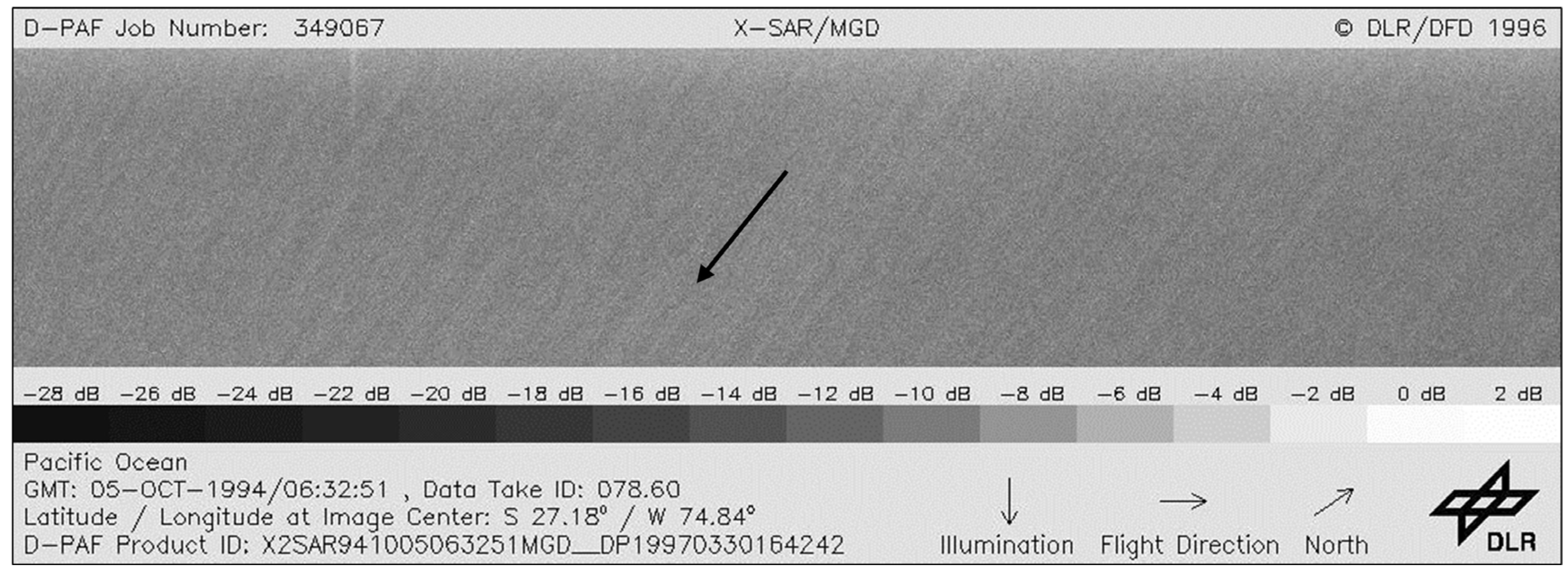
Quality control of the X-SAR data mainly excludes data that are significantly disrupted by rainfall, oil spills and other non-wind features [14]. Figure 1 shows an example of X-SAR data acquired over the Pacific Ocean for which only wind-related sea surface features are present. All of the selected X-SAR images are similar to this example.
Figure 1.
An example of X-band Synthetic Aperture Radar (X-SAR) data acquired over the Pacific Ocean (source: German Aerospace Center). The black arrow parallel to the linear wind streaks indicates the wind direction without 180° ambiguity.
Figure 1.
An example of X-band Synthetic Aperture Radar (X-SAR) data acquired over the Pacific Ocean (source: German Aerospace Center). The black arrow parallel to the linear wind streaks indicates the wind direction without 180° ambiguity.
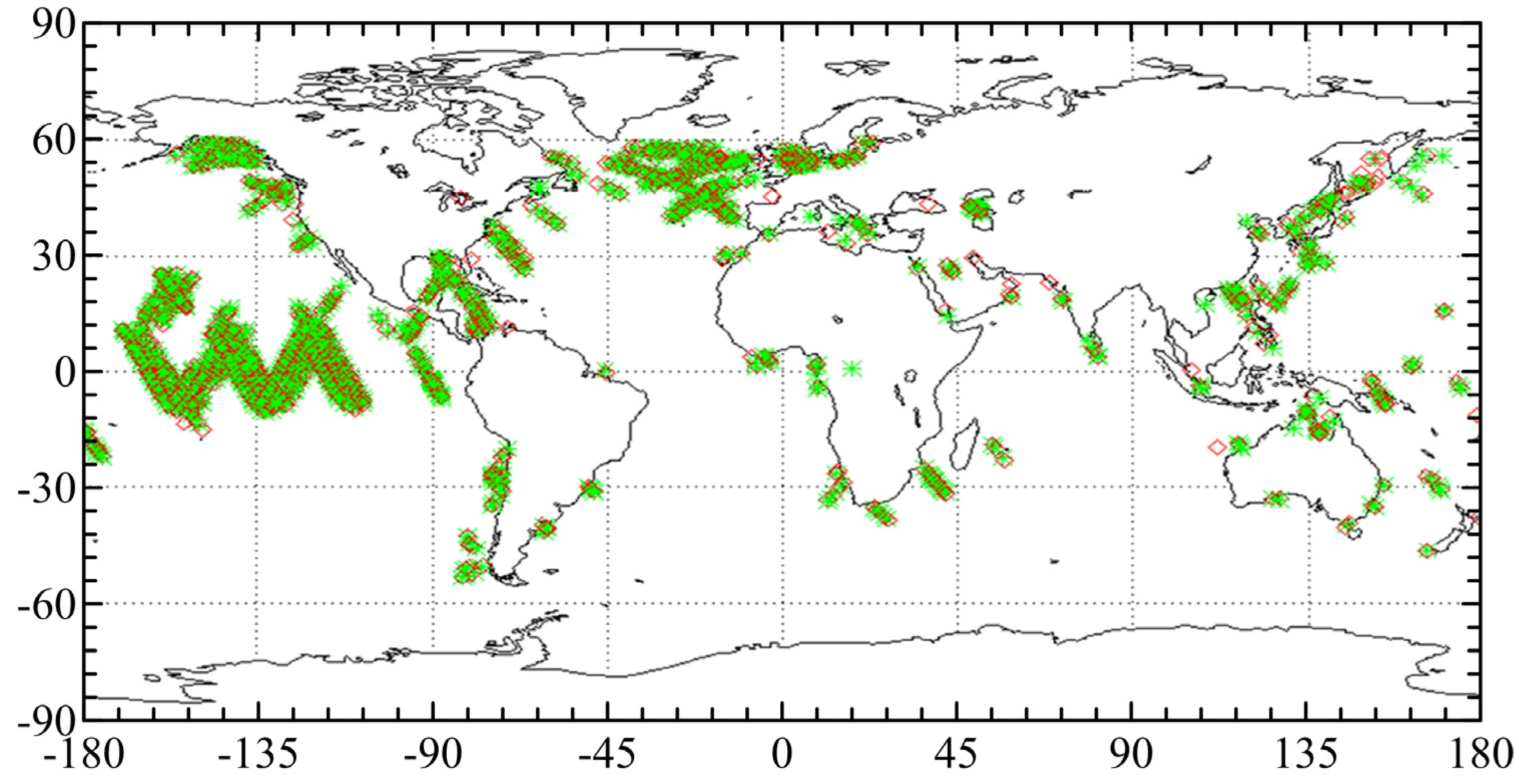
The entire dataset of the 2465 X-SAR images are randomly divided into two groups, which are used as two independent tuning datasets to verify the stability of the determined parameters in the GMF. The locations of the X-SAR data of the two datasets are shown in Figure 2, which are marked by red blocks and green stars, respectively.
Figure 2.
Schematic of the locations of the 2465 X-SAR images used for developing the Geophysical Model Function (GMF). The red and green marks represent the two independent datasets.
Figure 2.
Schematic of the locations of the 2465 X-SAR images used for developing the Geophysical Model Function (GMF). The red and green marks represent the two independent datasets.

2.2. ECMWF ERA–Interim Reanalysis Wind Field Data
The ECMWF ERA-Interim reanalysis wind data [15] that are spatially and temporally collocated with the X-SAR data are used as the tuning dataset. The 6-hour synoptic ERA-Interim reanalysis wind data has a spatial resolution of 0.75°. To obtain the wind field information corresponding to the center of the X-SAR image, the kriging method is used to interpolate the ERA-Interim data to a 0.25° × 0.25° grid.
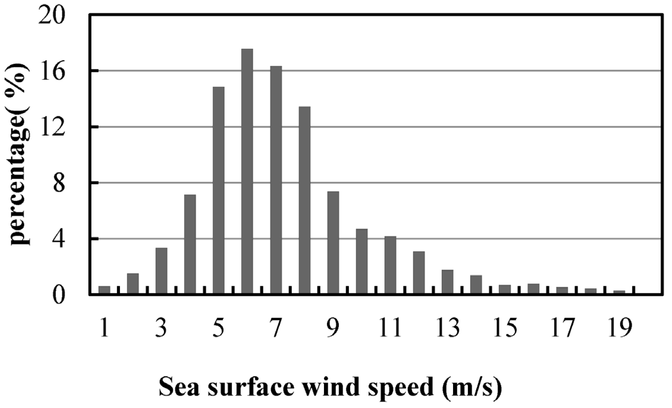
Figure 3 shows the histogram of the ERA-Interim sea surface wind speed collocated with the X-SAR data. The distribution of the model data suggests that most of the wind speeds are in the range of 3–12 m/s, which is consistent with surface wind speed distributions over the sea [16].
Figure 3.
Histogram of the ECMWF ERA-Interim reanalysis wind speeds collocated with the X-SAR data.

2.3. ERS-1/SCAT Data
2.4. Buoy Data
The in situ buoy data are accessed from the National Oceanographic Center (NODC) of NOAA. A total of 63 buoy records are selected to validate the sea surface wind fields retrieved from the X-SAR images in April and October, 1994. Most of the buoy anemometers are installed at a height of 5 m. Therefore, the wind speeds from the 5-m anemometers are converted to wind speeds at a standard height of 10 m, where SAR generally measures the sea surface wind speed. The following power-law wind profile [19] is used in this study.
where is the wind speed at height and and are the known wind speedand height, respectively. The exponent is approximately 0.10 [19] over the open sea.
3. Development of the SIRX-MOD Model
In this section, the development a non-linear GMF for the X-SAR data to retrieve the sea surface wind field is presented. The model is called SIRX-MOD.
3.1. Detailed Investigation of the Characteristics of X-SAR NRCS
The resonant Bragg wave number follows the relation (where represents the radar wavenumber). As the radar wavenumber , the X-band Bragg waves lie between the resonant wavenumbers at the C- and Ku-bands. Recent research [13] indicated that the overall X-band NRCS of TS-X and TD-X is similar to the simulated C- and Ku-band radar NRCS values. To date, the C-band SAR-based sea surface wind field retrieval algorithm is mainly adopted from CMOD4 [20], CMOD5 [21] and CMOD-IFR2 [17] GMFs that were originally developed for scatterometer data. The CMOD-IFR2 model function, which is applied to the ERS-1/2 scatterometer offline products, is obtained from the ECMWF, ERS/SCAT data and buoy data. When the wind speed is less than 20 m/s, the wind speed results retrieved from CMOD-IFR2 are consistent with CMOD4 and CMOD5, whereas the discrepancies among these GMFs exist at high wind speeds. Because the C-band GMFs of CMOD5, CMOD5.N and CMOD_IFR2 mainly have discrepancies for high wind speeds, we assume that all three GMFs yield similar simulations. However, the number of coefficients of CMOD_IFR2 is less than that of CMOD5, which is therefore easier for determining coefficients to update the X-SAR wind retrieval algorithm, particularly when the tuning dataset is not sufficient to cover all the wind conditions. A recent study [22] compared the sea surface wind speeds retrieved using CMOD_IFR2, CMOD5 and CMOD5.N with measurements at the two weather platforms of Horns Rev and Egmond aan Zee. However, it reveals that CMOD_IFR2 performs slightly better than CMOD5 or CMOD5.N for retrieving sea surface wind speeds under 20 m/s in terms of bias. For these reasons, the updated X-SAR wind retrieval algorithm (SIRX-MOD) is based on CMOD_IFR2.
CMOD-IFR2 empirically relates the C-band radar NRCS to surface wind speed by a power law, which is expressed by the following logarithmic equation:
The model is detailed described in the Appendix.
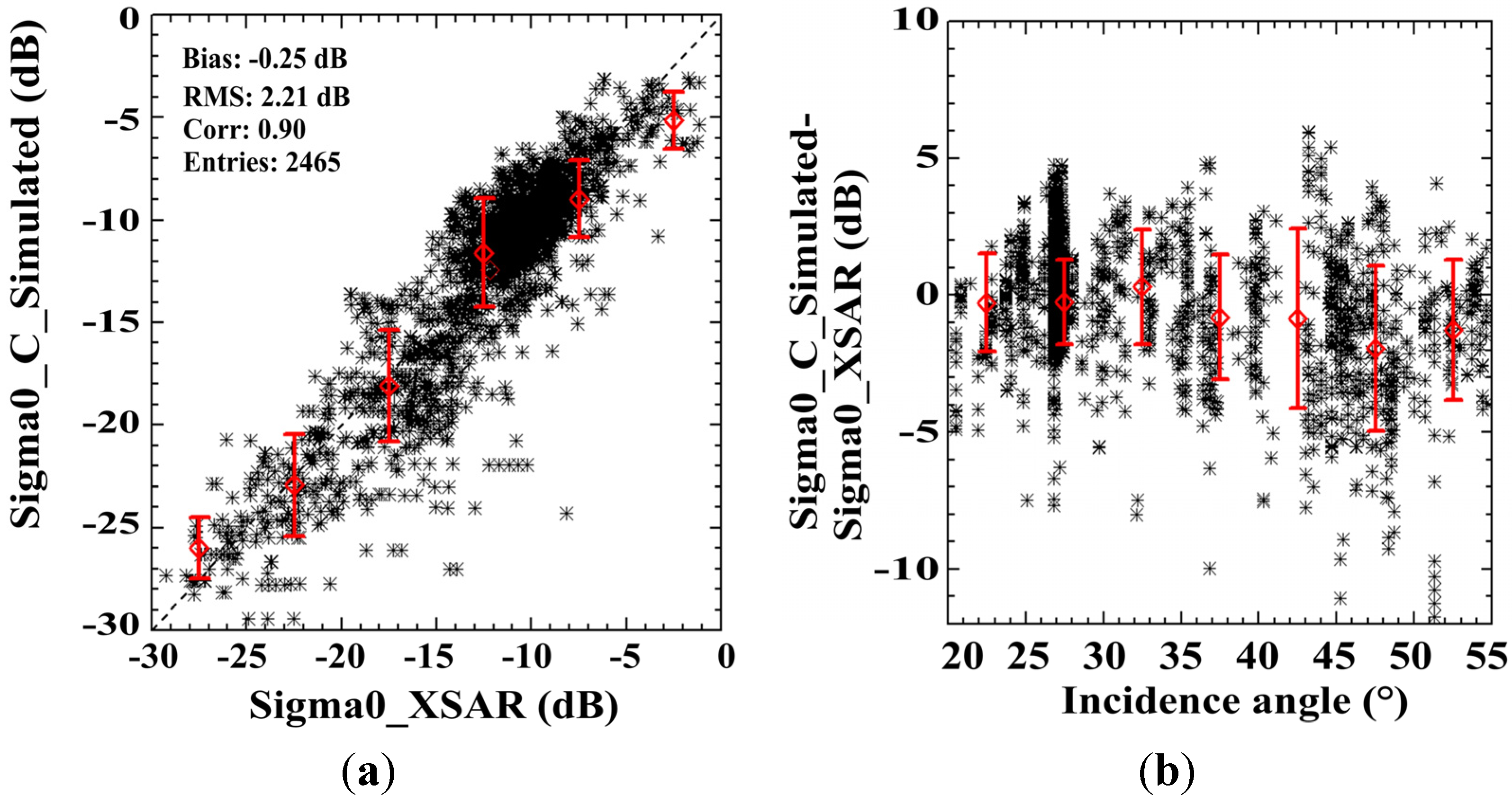
The sea surface wind speed and wind direction derived from the ERA-Interim model data and incidence angles of the X-SAR data are added to the CMOD_IFR2 model to simulate the C-band SAR NRCS, which is compared with the NRCS of the X-SAR data, as shown in Figure 4a. All the simulated C-band SAR NRCSs, sorted in ascending order of X-SAR NRCSs, are divided into 6 groups (5 dB intervals). The red error bars are plotted as the mean value ± standard deviation of every group of simulated NRCS. Similar to the finding in [13], the X-band sea surface backscatter intensity is slightly higher than that of the C-band by 0.25 dB. It appears that −10 dB is a turning point of the discrepancy between the C-band and X-band NRCSs. For NRCSs lower than −10 dB, the C-band and X-band NRCSs are very similar. However, when the value is higher than the threshold, the NRCS of the X-band is systematically higher than that of the C-band. A further analysis is the dependence of this discrepancy on the incidence angle, as shown in Figure 4b, in which the star represents every difference between the X-SAR NRCS and the CMOD-IFR2 simulation. All of the differences sorted in ascending order of the incidence angle are divided into 7 groups (5-degree intervals). The red error bars are plotted as the mean value ± standard deviation of every group of NRCS differences. For the incidence angles less than approximately 40°, the NRCSs of the X-band and C-band are similar. However, the value decreases for incidence angles larger than 40°.
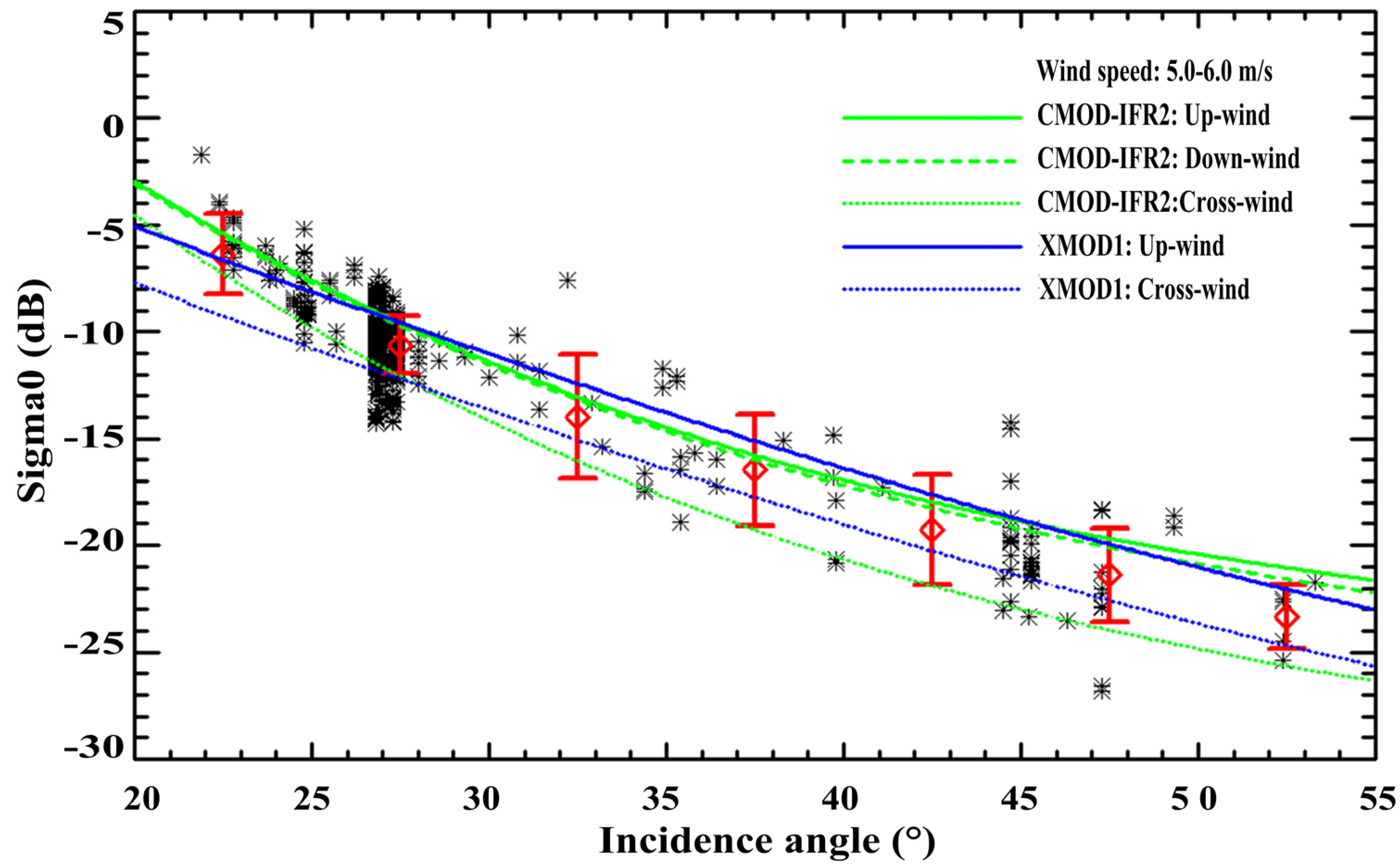
In Figure 5, the collocated X-SAR NRCS (asterisks) within the wind speed range is compared with the simulated C-band NRCS at various incidence angles. The simulation conducted by the X-band GMF XMOD1 is also superimposed for comparison. The solid, dashed and dotted curves are the simulated NRCS using different GMF models at the sea surface wind speed of 5.5 m/s for up-wind, down-wind and cross-wind, respectively. Notably, GMF XMOD1 assumes that there is no difference in the down-wind and up-wind NRCSs. The green and blue curves represent CMOD-IFR2 and XMOD1, respectively. The X-band NRCS simulated using the XMOD1 model agrees well with the X-SAR NRCS in the incidence angle range from 25° to 55°, whereas it significantly underestimates the X-band NRCS for incidence angles between 20° and 25°. However, the difference between up-wind and cross-wind conditions according to the linear XMOD1 is uniform, which does not depict the dependence of their differences (between up-wind and cross-wind) on incidence angles. Although the simulated C-band NRCS using CMOD-IFR2 is systematically lower than that of the X-band under such wind conditions, the trends of their dependences on the incidence angles are similar to the observations of the X-band SAR.
Figure 4.
Comparison of the simulated normalized radar cross sections (NRCSs) using CMOD-IFR2 and the X-SAR measurements. The red error bars are plotted as the mean value ± standard deviation of the differences between the simulation and observation. (a) A direct comparison of the simulated C-band NRCS by the CMOD-IFR2 and X-SAR measurements; and (b) the differences in NRCSs simulated using CMOD-IFR2 and X-SAR measurements at various incidence angles.

Figure 5.
Comparison among the NRCSs of CMOD-IFR2, XMOD1 and X-SAR.
3.2. Determining the Coefficients of SIRX-MOD
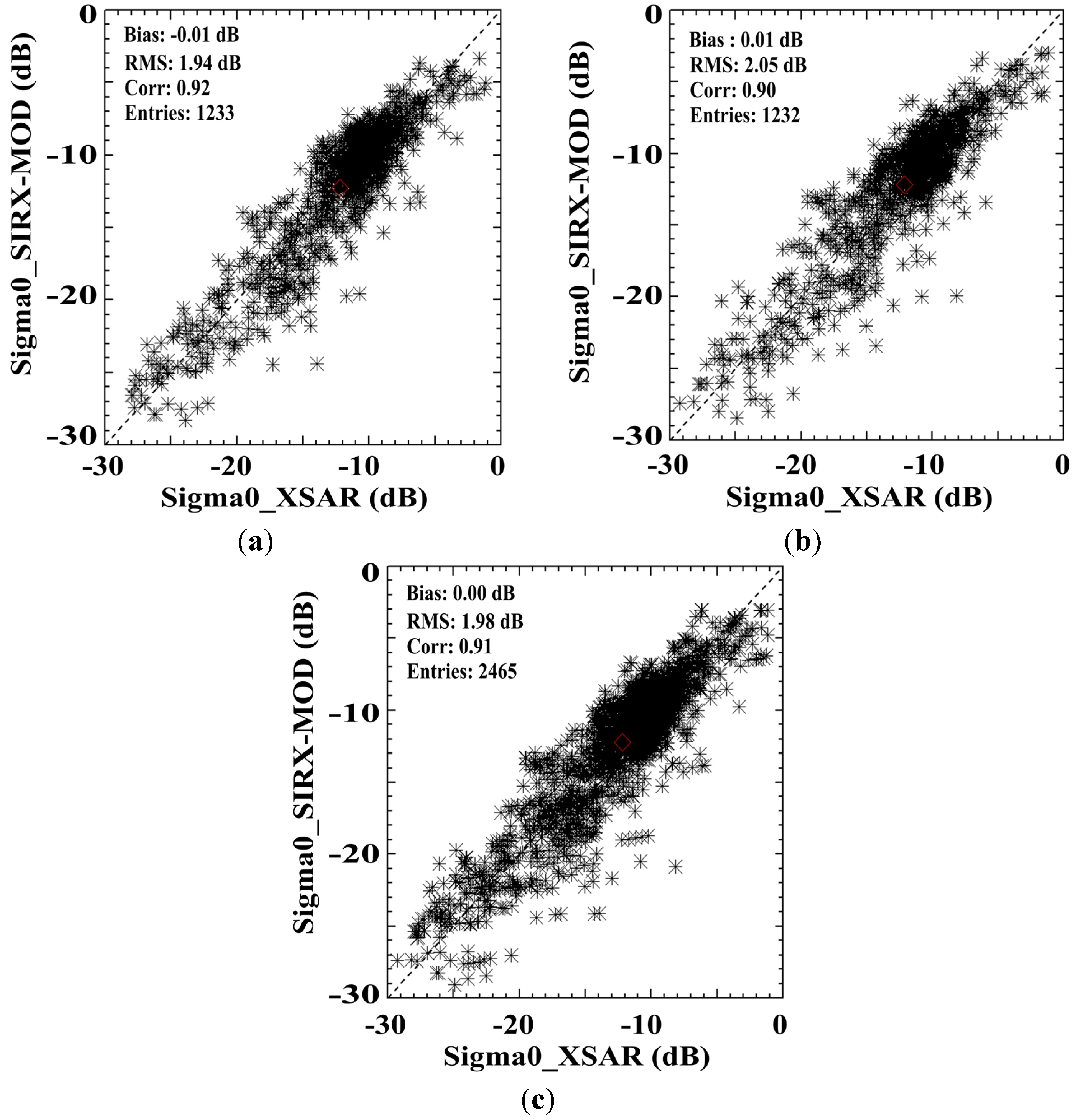
The entirety of the quality-controlled X-SAR data acquired over the ocean is used as the tuning dataset for determining the coefficients in SIRX-MOD. However, a practical problem is whether the tuning dataset is sufficient to obtain stable coefficients in X-SAR GMF. Therefore, we first divide the entire dataset into two random groups, which are used separately to determine the coefficients in formula (2) to verify the stability of the tuning process. Figure 6a,b are comparisons of the simulated X-band NRCS using SIRX-MOD with the observations using the two groups of data pairs. The two comparisons yield very similar verification results, with root mean square (RMS) errors of 1.94 dB and 2.05 dB, respectively. The coefficients are listed in Table 1. Although the two sets of coefficients are slightly different, the similar statistical parameters derived from the verification suggest that the dataset is somehow sufficient to determine the coefficients. We therefore use the entire dataset to ultimately determine the coefficients in SIRX-MOD, which are listed in the third column of Table 1.
Figure 6.
Comparison between the NRCS simulated by the SIRX-MOD model and X-SAR observations for (a) dataset 1; (b) dataset 2 and (c) all datasets.
Figure 6.
Comparison between the NRCS simulated by the SIRX-MOD model and X-SAR observations for (a) dataset 1; (b) dataset 2 and (c) all datasets.


| Coefficients | Dataset 1 | Dataset 2 | All Data |
|---|---|---|---|
| c1 | −2.4429 | −2.4558 | −2.4801 |
| c2 | −1.5423 | −1.4817 | −1.4403 |
| c3 | 0.30494 | 0.35853 | 0.36764 |
| c4 | −0.02195 | −0.02418 | −0.02125 |
| c5 | 0.42573 | 0.43027 | 0.44294 |
| c6 | 0.2051 | 0.2289 | 0.1933 |
| c7 | −0.010682 | −0.015719 | −0.011386 |
| c8 | 0.0816655 | 0.073983 | 0.091643 |
| c9 | 0.03501 | 0.05117 | 0.04692 |
| c10 | 0.06986 | 0.04964 | 0.06168 |
| c11 | 0.00677 | 0.01114 | 0.00616 |
| c12 | −0.08416 | −0.08115 | −0.08855 |
| c13 | −0.08414 | −0.05046 | −0.07911 |
| c14 | 0.42894 | 0.41735 | 0.41259 |
| c15 | 0.13599 | 0.12919 | 0.13407 |
| c16 | −0.01921 | −0.0774 | −0.02197 |
| c17 | 0.06424 | 0.0014 | 0.07358 |
| c18 | −0.0429 | −0.0851 | −0.0597 |
| c19 | 0.2788 | 0.2483 | 0.2169 |
| c20 | −0.04032 | −0.08538 | −0.04056 |
| c21 | −0.09517 | −0.06814 | −0.07539 |
| c22 | 0.1045 | 0.1934 | 0.0181 |
| c23 | 0.02493 | 0.02054 | 0.02692 |
| c24 | 0.11474 | 0.19205 | 0.15508 |
| c25 | 0.03833 | 0.05896 | 0.03500 |
3.3. Simulation of SIRX-MOD
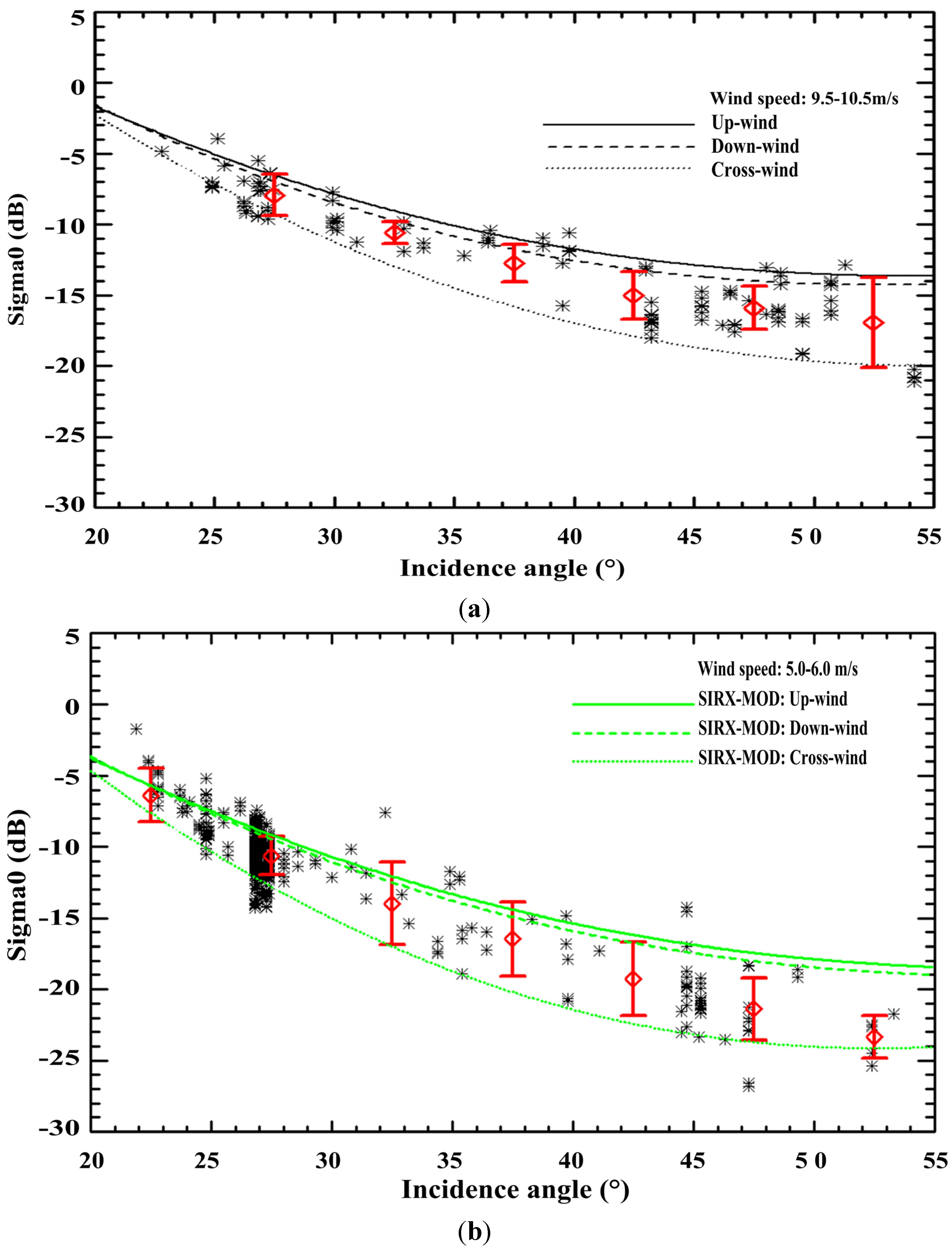
Simulations of SIRX-MOD are run to determine the dependence of the X-band NRCS on the incidence angles and sea surface wind field. In Figure 7a, the collocated X-SAR NRCS (asterisks) in the wind speed range from 9.5 m/s to 10.5 m/s is comparable to the simulated NRCS using the SIRX-MOD model at various incidence angles for up-wind, down-wind and cross-wind conditions. The NRCS simulated using the SIRX-MOD model agrees well with the X-SAR NRCS.
Figure 7b shows the other simulation for the sea surface wind speed of 5.5 m/s, which matches the diagram shown in Figure 5. The green solid, dashed and dotted curves are the simulated NRCS using the SIRX-MOD model for up-wind, down-wind and cross-wind conditions, respectively. The NRCS simulated using the SIRX-MOD model agrees well with the X-SAR observations, although the difference in the NRCSs between the up-wind and cross-wind conditions of real X-SAR data is larger than the prediction of SIRX-MOD for incidence angles greater than 25°.
Figure 7.
NRCS values simulated using the SIRX-MOD model for various incidence angles at sea surface wind speeds of (a) 10 m/s and (b) 5.5 m/s. The red error bars are plotted as the mean value ± standard deviation of the X-SAR NRCS.
Figure 7.
NRCS values simulated using the SIRX-MOD model for various incidence angles at sea surface wind speeds of (a) 10 m/s and (b) 5.5 m/s. The red error bars are plotted as the mean value ± standard deviation of the X-SAR NRCS.

The dependence of the NRCS on wind direction is simulated using the SIRX-MOD model for various wind speeds, as shown in Figure 8. The statistical results suggest that the collocation data pairs have the largest range of surface wind speeds (4.5 m/s to 5.5 m/s) at an incidence angle of 27°. Therefore, Figure 8 shows the periodic behaviors at an incidence angle of 27°. The difference between the NRCS in up-wind and down-wind scenarios increases slightly with increasing wind speed. When the sea surface wind speed decreases to 5 m/s, there is no evident difference in the NRCS between up-wind and down-wind scenarios. When the wind speed reaches 20 m/s, the difference is as high as 0.9 dB.
Figure 8.
NRCS values simulated using the SIRX-MOD model for various wind directions with an incidence angle of 27°.
Figure 8.
NRCS values simulated using the SIRX-MOD model for various wind directions with an incidence angle of 27°.
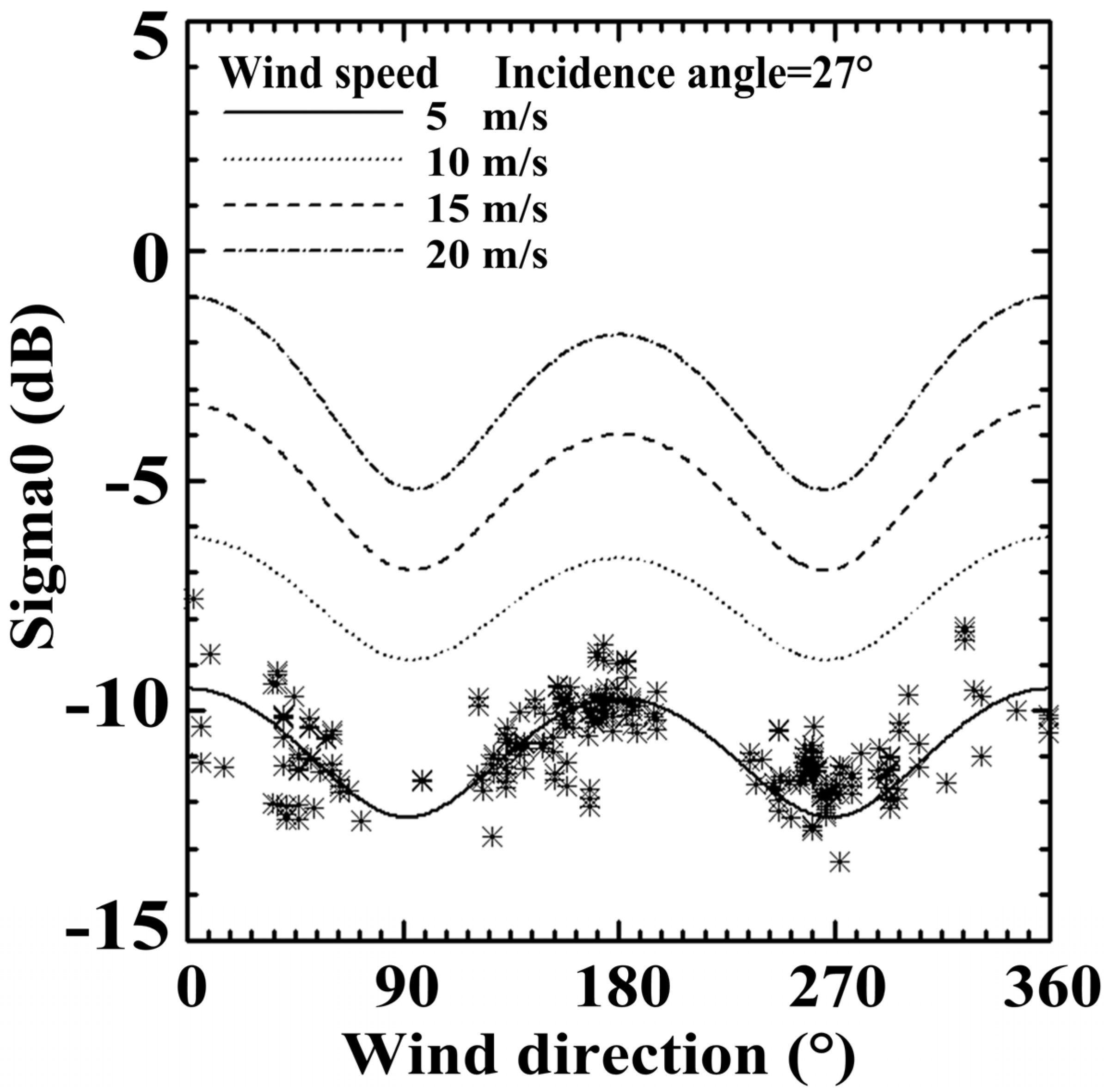
The asterisks shown in Figure 8 are the X-SAR observations in the incidence angle of 27°. We can find that the data obtained by X-SAR do not distribute regularly. Therefore, it is not possible to draw any functions independently. Thus, we select a developed GMF, e.g., CMOD-IFR2 used in this study as a prototype to find a solution. The simulation using the developed SIRX-MOD shown in the figure suggests that it could depict well the behavior of the X-SAR observations.
3.4. Validation of the SIRX-MOD Model
Because the coefficients of SIRX-MOD are used for the collocation data pairs of X-SAR and the ERA-Interim reanalysis wind data, SIRX-MOD is validated by comparing the retrieved sea surface wind speed with other independent observations, i.e., the measurements of ERS-1/SCAT and in situ buoys. The criteria of collocating the SX-SAR data with the ERS-1/SCAT and buoy data are a spatial distance of less than 200 km and a temporal difference of less than one hour.
To retrieve the sea surface wind speed using any GMF from the SAR data, a priori wind direction is important. When the collocation criteria mentioned above are used, there are few data pairs available. Therefore, the ERS-1/SCAT and buoy wind direction information are used for the wind speed retrieval from X-SAR. A sub-scene size of 2 km × 2 km derived from X-SAR data is used for the retrieval.
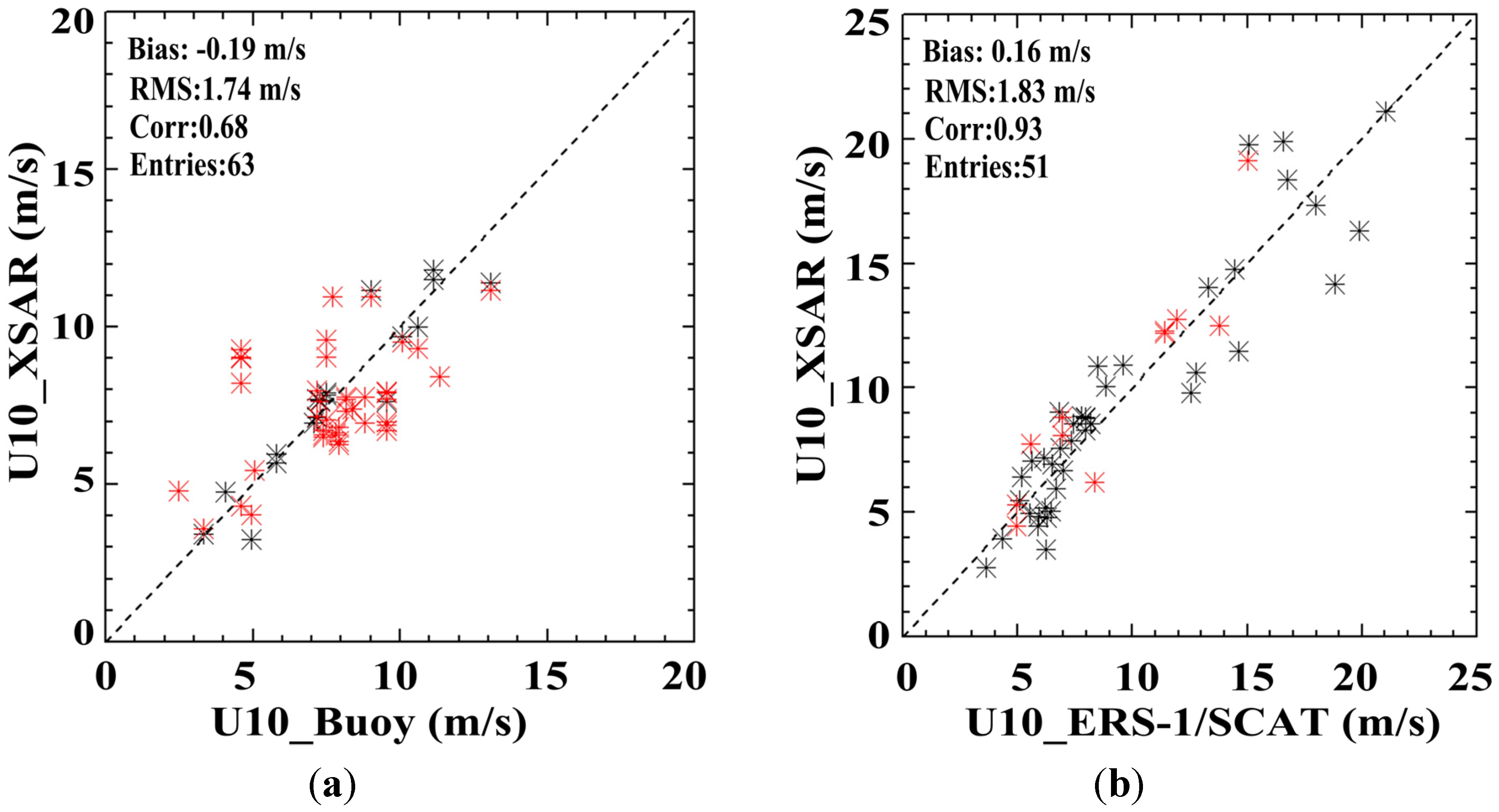
In total, 63 buoy measurements meet the collocation criteria. The comparison is shown in Figure 9a, where the red signs indicate the data pairs with a collocation distance of less than 100 km. The bias, RMS and correlation are 0.13m/s, 1.63m/s and 0.68, respectively. The figure indicates a reasonable agreement with the buoy measurements. However, when the sea surface wind speed is above 10 m/s, the retrieved SAR wind speeds tend to be higher than those of the buoy measurements. Based on the collocation criteria mentioned, 51 data pairs of X-SAR and ERS-1/SCAT are obtained. Figure 9b shows the comparison results. The bias, RMS and correlation of the comparison are 0.16 m/s, 1.83 m/s and 0.93, respectively. Although the collocations of X-SAR, in situ buoys and ERS-1/SCAT are quite limited, the validation results with a bias of less 0.2 m/s and a RMS of less than 2.0 m/s suggest that SIRX-MOD yields a reasonable retrieval.
Figure 9.
Validation of the SIRX-MOD model through a comparison with (a) in situ buoy measurements and (b) ERS-1/SCAT measurements. The red signs indicate the collocation distance between the X-SAR data and the buoy or ERS-1/SCAT is less than 100 km.
Figure 9.
Validation of the SIRX-MOD model through a comparison with (a) in situ buoy measurements and (b) ERS-1/SCAT measurements. The red signs indicate the collocation distance between the X-SAR data and the buoy or ERS-1/SCAT is less than 100 km.
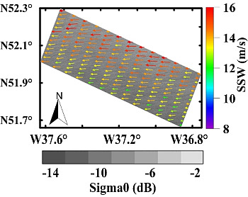
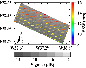
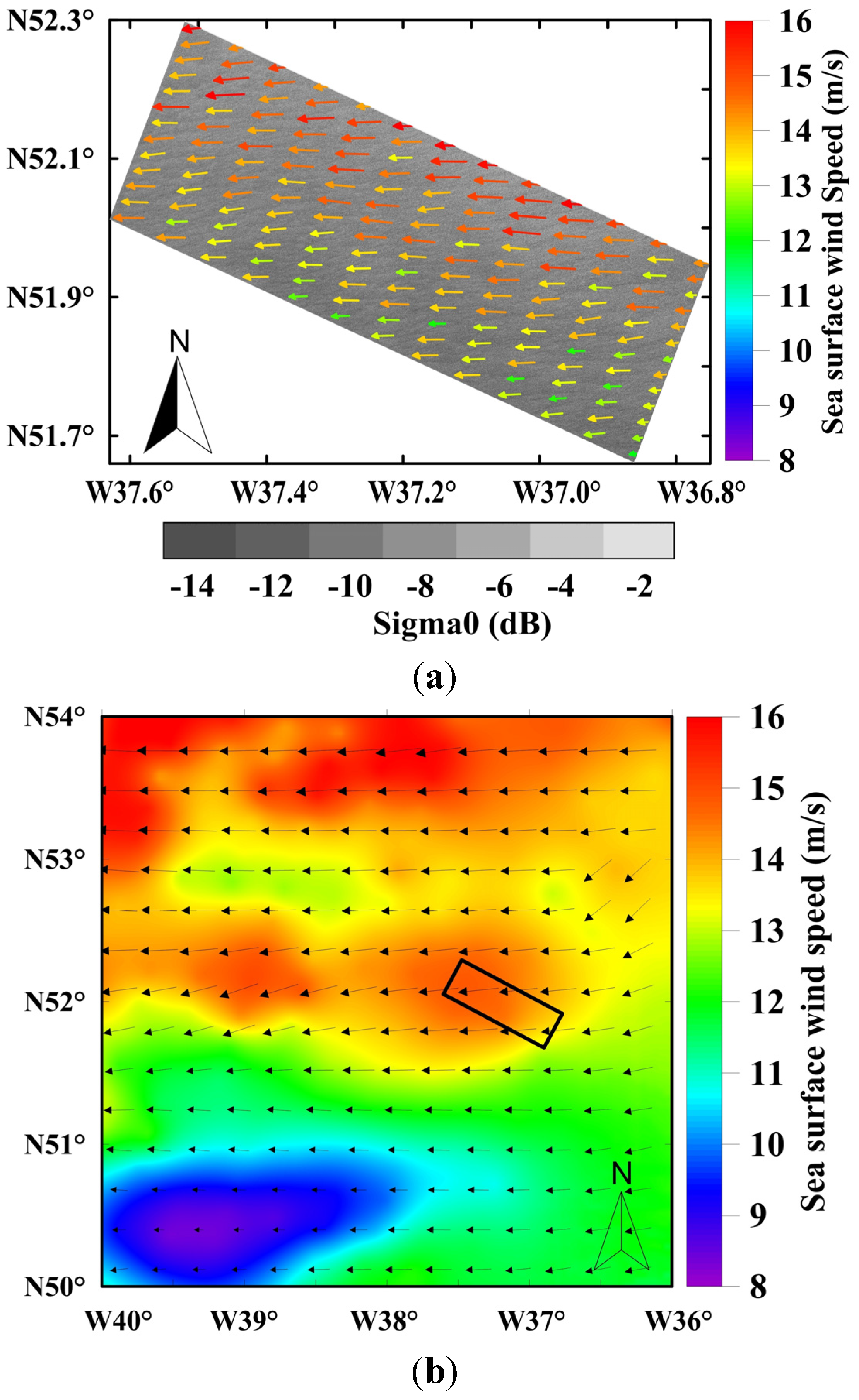
X-SAR data acquired over the Atlantic Ocean on Oct. 6, 1994 at 12:42 GMT are selected to retrieve the sea surface wind field using SIRX-MOD, as shown in Figure 10a. The large-coverage ERS-1/SCAT measurements are shown in Figure 10b. The FFT method [23] is used for deriving the wind direction from the X-SAR data, as wind streaks are clearly visible. The remaining 180° ambiguity in the wind direction is resolved using the ERS-1/SCAT measurements. The retrieved X-SAR sea surface wind speed varies between 12 m/s and 16 m/s, indicating a significant spatial variation, while the ERS-1/SCAT measurements show a homogeneous sea surface wind field due to the low spatial resolution of 25 km. This example demonstrates the need for a SAR sea surface wind retrieval algorithm, which could yield high spatial resolution sea surface winds on a kilometer scale.
Figure 10.
The application of the SIRX-MOD model to X-SAR data. (a) Sea surface wind field retrieved using the SIRX-MOD model with X-SAR data acquired on October 6, 1994 at 12:42 GMT over the Atlantic Ocean; (b) Sea surface wind field from ERS-1/SCAT obtained on October 6, 1994 at 13:27 GMT over the Atlantic Ocean. The black rectangle indicates the area where the X-SAR scene was obtained.

4. Conclusion
In the study, we revisited the X-SAR sea surface wind retrieval algorithm using the entire dataset acquired by X-SAR.
We compare the simulated C-band NRCS using the CMOD_IFR2 model with X-SAR observations. Regardless of the overall comparison or single comparison at a particular wind speed range, the C-band NRCS shows a pattern similar to the X-band observations, which should be attributed to the similar resonant Bragg wave numbers of the C- and X-bands. We therefore use a C-band GMF as a prototype to update the X-SAR sea surface wind retrieval algorithm.
All of the X-SAR data are randomly grouped to determine the coefficients of SIRX-MOD. The respective coefficients and the statistical parameters obtained in the two verification processes are quite similar. This finding indicates that the available dataset could yield a stable tuning result. The final coefficients in SIRX-MOD are determined using all of the X-SAR data and their collocated ERA-Interim reanalysis wind data.
We further use independent data sources of in situ buoy measurements and ERS-1/SCAT retrievals to validate SIRX-MOD. The comparison result with the buoys yields a bias of 0.13 m/s and a RMS error of 1.63 m/s. Although the statistical parameters in terms of bias and RMS values of 0.16 m/s and 1.83 m/s, respectively, obtained from the comparison with the ERS-1/SCAT retrieval are slightly higher than those of the comparison with the buoy, the high correlation of 0.93 indicates that we could obtain reasonable sea surface wind speeds from X-SAR data using SIRX-MOD.
A comparison of C- and X-band SAR NRCSs is still needed. In this study, CMOD-IFR2 is used to simulate the C-band SAR NRCS. In fact, SIR-C/X-SAR simultaneously acquires the C- and L-band SAR data and X-band data. However, we are still attempting to obtain the full dataset of SIR-C. In the future, we will focus on more realistic analyses of the radar backscatter of the three frequencies at the sea surface.
Appendix
The CMOD-IFR2 model is as follows:
where is the NRCS, is the angle between the radar look direction and wind direction, W is the wind velocity and is the incidence angle of the radar.
| c1 | −2.437597 |
| c2 | −1.5670307 |
| c3 | 0.3708242 |
| c4 | −0.040590 |
| c5 | 0.404678 |
| c6 | 0.188397 |
| c7 | −0.027262 |
| c8 | 0.064650 |
| c9 | 0.054500 |
| c10 | 0.086350 |
| c11 | 0.055100 |
| c12 | −0.058450 |
| c13 | −0.096100 |
| c14 | 0.412754 |
| c15 | 0.121785 |
| c16 | −0.024333 |
| c17 | 0.072163 |
| c18 | −0.062954 |
| c19 | 0.015958 |
| c20 | −0.069514 |
| c21 | −0.062945 |
| c22 | 0.035538 |
| c23 | 0.023049 |
| c24 | 0.074654 |
| c25 | −0.014713 |
Acknowledgments
The authors would like to thank the DLR for kindly providing the X-SAR data. The ERA-Interim data, ERS/SCAT data, and in situ buoy data were freely downloaded from ECMWF (http://apps.ecmwf.int/datasets/data/interim_full_daily/), IFREMER (ftp://ftp.ifremer.fr/ifremer/cersat/products/swath/scatterometers/wnf/) and the NDBC (http://www.ndbc.noaa.gov/data/historical/). The study was partially supported by grants awarded to Ren and Li by the NSFC program (no. 41471309) and the “100 Talents Program” of the Chinese Academy of Sciences (no. Y4S00400CX) and to Zhou by the NSFC program (no. 41431179 and no. 41162011).
Author Contributions
Yongzheng Ren and Xiao-Ming Li came up with the original idea for the study. Yongzheng Ren processed and analyzed the data. Guoqing Zhou significantly contributed to the discussion of the results. Xiao-Ming Li drafted the manuscript, which was revised by all of the authors. All of the authors read and approved the final manuscript.
Conflicts of Interest
The authors declare no conflict of interest.
References
- Schmullius, C.C.; Evans, D.L. Synthetic aperture radar (SAR) frequency and polarization requirements for applications in ecology, geology, hydrology, and oceanography: A tabular status quo after SIR-C/X-SAR. Int. J. Remote Sens. 1997, 18, 2713–2722. [Google Scholar] [CrossRef]
- Evans, D.L. Spaceborne imaging radar-C/X-band synthetic aperture radar (SIR-C/X-SAR): A look back on the tenth anniversary. IEE Proc. Radar Son. Navig. 2006, 153, 81–85. [Google Scholar] [CrossRef]
- Monaldo, F.M.; Beal, R.C. Comparison of Sir-C SAR wavenumber spectra with wam model predictions. J. Geophys. Res.: Ocean. 1998, 103, 18815–18825. [Google Scholar] [CrossRef]
- Melsheimer, C.; Bao, M.Q.; Alpers, W. Imaging of ocean waves on both sides of an atmospheric front by the SIR-C/X-SAR multifrequency synthetic aperture radar. J. Geophys. Res.: Ocean. 1998, 103, 18839–18849. [Google Scholar] [CrossRef]
- Ufermann, S.; Romeiser, R. A new interpretation of multifrequency/multipolarization radar signatures of the Gulf Stream front. J. Geophys. Res.: Ocean. 1999, 104, 25697–25705. [Google Scholar] [CrossRef]
- Jameson, A.R.; Li, F.K.; Durden, S.L.; Haddad, Z.S.; Holt, B.M.; Fogarty, T.; Im, E.; Moore, R.K. SIR-C/X-SAR observations of rain storms. Remote Sens. Environ. 1997, 59, 267–279. [Google Scholar] [CrossRef]
- Moore, R.K.; Mogili, A.; Fang, Y.; Beh, B.; Ahamad, A. Rain measurement with SIR-C/X-SAR. Remote Sens. Environ. 1997, 59, 280–293. [Google Scholar] [CrossRef]
- Melsheimer, C.; Alpers, W.; Gade, M. Investigation of multifrequency/multipolarization radar signatures of rain cells over the ocean using SIR-C/X-SAR data. J. Geophys. Res.: Ocean. 1998, 103, 18867–18884. [Google Scholar] [CrossRef]
- Gade, M.; Alpers, W.; Huhnerfuss, H.; Masuko, H.; Kobayashi, T. Imaging of biogenic and anthropogenic ocean surface films by the multifrequency/multipolarization SIR-C/X-SAR. J. Geophys. Res.: Ocean. 1998, 103, 18851–18866. [Google Scholar] [CrossRef]
- Migliaccio, M.; Gambardella, A.; Tranfaglia, M. SAR polarimetry to observe oil spills. IEEE Trans. Geosci. Remote Sens. 2007, 45, 506–511. [Google Scholar] [CrossRef]
- Nunziata, F.; Gambardella, A.; Migliaccio, M. On the Mueller scattering matrix for SAR sea oil slick observation. IEEE Trans. Geosci. Remote Sens. 2008, 5, 691–695. [Google Scholar] [CrossRef]
- Ren, Y.Z.; Lehner, S.; Brusch, S.; Li, X.M.; He, M.X. An algorithm for the retrieval of sea surface wind fields using X-band TerraSAR-X data. Int. J. Remote Sens. 2012, 33, 7310–7336. [Google Scholar] [CrossRef]
- Li, X.M.; Lehner, S. Algorithm for sea surface wind retrieval from TerraSAR-X and TanDEM-X data. IEEE Trans. Geosci. Remote Sens. 2014, 52, 2928–2939. [Google Scholar] [CrossRef]
- Clemente-Colon, P.; Yan, X.H. Low-backscatter ocean features in synthetic aperture radar imagery. Johns Hopkins Apl Tech. Dig. 2000, 21, 116–121. [Google Scholar]
- Dee, D.P.; Uppala, S.M.; Simmons, A.J.; Berrisford, P.; Poli, P.; Kobayashi, S.; Andrae, U.; Balmaseda, M.A.; Balsamo, G.; Bauer, P.; et al. The era-interim reanalysis: Configuration and performance of the data assimilation system. Q. J. R. Meteorol. Soc. 2011, 137, 553–597. [Google Scholar] [CrossRef]
- Monahan, A.H. The probability distribution of sea surface wind speeds. Part 1: Theory and seawinds observations. J. Clim. 2006, 19, 497–520. [Google Scholar] [CrossRef]
- Quilfen, Y.; Chapron, B.; Elfouhaily, T.; Katsaros, K.; Tournadre, J. Observation of tropical cyclones by high-resolution scatterometry. J. Geophys. Res.: Ocean. 1998, 103, 7767–7786. [Google Scholar] [CrossRef]
- Quilfen, Y. Ers-1 scatterometer off-line products—Calibration validation results and case-studies. In Proceedings of the 1993 International Geoscience and Remote Sensing Symposium, Tokyo, Japan, 18–21 August 1993; pp. 1750–1752.
- Hsu, S.A.; Meindl, E.A.; Gilhousen, D.B. Determining the power-law wind-profile exponent under near-neutral stability conditions at sea. J. Appl. Meteorol. 1994, 33, 757–765. [Google Scholar] [CrossRef]
- Stoffelen, A.; Anderson, D. Scatterometer data interpretation: Estimation and validation of the transfer function CMOD4. J. Geophys. Res.: Ocean. 1997, 102, 5767–5780. [Google Scholar] [CrossRef]
- Hersbach, H.; Stoffelen, A.; de Haan, S. An improved C-band scatterometer ocean geophysical model function: CMOD5. J. Geophys. Res.: Ocean. 2007, 112, 1–18. [Google Scholar] [CrossRef]
- Charlotte, H.; Mouche, A.; Badger, M.; Bingöl, F.; Karagali, I.; Driesenaar, T.; Stoffelen, A.D.; Peña, A.; Longépé, N. Offshore wind climatology based on synergetic use of Envisat ASAR, ASCAT and QuikSCAT. Remote Sens. Environ. 2015, 156, 247–263. [Google Scholar] [Green Version]
- Lehner, S.; Horstmann, J.; Koch, W.; Rosenthal, W. Mesoscale wind measurements using recalibrated ERS SAR images. J. Geophys. Res.: Ocean. 1998, 103, 7847–7856. [Google Scholar] [CrossRef]
© 2015 by the authors; licensee MDPI, Basel, Switzerland. This article is an open access article distributed under the terms and conditions of the Creative Commons Attribution license (http://creativecommons.org/licenses/by/4.0/).
Share and Cite
MDPI and ACS Style
Ren, Y.; Li, X.-M.; Zhou, G. Sea Surface Wind Retrievals from SIR-C/X-SAR Data: A Revisit. Remote Sens. 2015, 7, 3548-3564. https://doi.org/10.3390/rs70403548
AMA Style
Ren Y, Li X-M, Zhou G. Sea Surface Wind Retrievals from SIR-C/X-SAR Data: A Revisit. Remote Sensing. 2015; 7(4):3548-3564. https://doi.org/10.3390/rs70403548
Chicago/Turabian StyleRen, Yongzheng, Xiao-Ming Li, and Guoqing Zhou. 2015. "Sea Surface Wind Retrievals from SIR-C/X-SAR Data: A Revisit" Remote Sensing 7, no. 4: 3548-3564. https://doi.org/10.3390/rs70403548