Article

Temporal Upscaling and Reconstruction of Thermal Remotely Sensed Instantaneous Evapotranspiration

1
State Key Laboratory of Remote Sensing Science, Research Center for Remote Sensing and GIS, and School of Geography, Beijing Normal University, No.19, Xinjiekouwai Street, 100875 Beijing, China
2
Information Technology Department, National Library of China, No. 33, Zhongguancun Nandajie, 100081 Beijing, China
3
Yangzhou Environmental Monitoring Center, No.446, Yangzijiangbei Road, 225007 Yangzhou, China
4
Department of Civil and Environmental Engineering and Water Resource Research Center, University of Hawaii at Manoa, Honolulu, HI 96822, USA
*
Author to whom correspondence should be addressed.
Remote Sens. 2015, 7(3), 3400-3425; https://doi.org/10.3390/rs70303400
Submission received: 13 January 2015 / Revised: 28 February 2015 / Accepted: 17 March 2015 / Published: 23 March 2015

Abstract

:
Currently, thermal remote sensing-based evapotranspiration (ET) models can only calculate instantaneous ET at the time of satellite overpass. Five temporal upscaling methods, namely, constant evaporative fraction (ConEF), corrected ConEF (CorEF), diurnal evaporative fraction (DiEF), constant solar radiation ratio (SolRad), and constant reference evaporative fraction (ConETrF), were selected to upscale the instantaneous ET to daily values. Moreover, five temporal reconstruction approaches, namely, data assimilation (ET_EnKF and ET_SCE_UA), surface resistance (ET_SR), reference evapotranspiration (ET_ETrF), and harmonic analysis of time series (ET_HANTS), were used to produce continuous daily ET with discrete clear-sky daily ET values. For clear-sky daily ET generation, SolRad and ConETrF produced the best estimates. In contrast, ConEF usually underestimated the daily ET. The optimum method, however, was found by combining SolRad and ConETrF, which produced the lowest root-mean-square error (RMSE) values. For continuous daily ET production, ET_ETrF and ET_SCE_UA performed the best, whereas the ET_SR and ET_HANTS methods had large errors. The annual ET distributions over the Beijing area were calculated with these methods. The spatial ET distributions from ET_ETrF and ET_SCE_UA had the same trend as ETWatch products, and had a smaller RMSE when compared with ET observations derived from the water balance method.

Graphical Abstract

1. Introduction

Evapotranspiration (ET) is one of the most important components of surface energy budgets and hydrologic cycles. Flux observation networks (e.g., FluxNet) and enhanced experiments (e.g., HiWATER) have been set up to monitor long-term surface heat fluxes over different kinds of land cover [1,2,3]. However, in situ measurements are expensive and difficult to extend to continental scales. Thus, models have been developed to map ET over continental scales based on remotely sensed information [4,5,6,7,8,9,10,11]. Unfortunately, thermal remotely sensed models can only detect a snapshot of ET spatial distributions at the time of satellite overpass. The snapshot of the ET map cannot satisfy practical applications, such as, irrigation judgment, and water resource planning and management. To satisfy such applications, the instantaneous ET needs to be upscaled to daily values for clear-sky days. Moreover, continuous daily ET values should be generated with temporal reconstruction approaches to fulfill long-term hydrologic requirements.
There are many methods to upscale instantaneous ET to daily values. The most popular approach is the constant evaporative fraction (EF) method, which assumes that EF (EF is defined as the ratio of latent heat flux and available energy) is constant during the daytime [12]. Thus, the daily ET can be obtained with daily available energy (difference of net radiation, Rn, and soil heat flux, G0) and remotely sensed instantaneous EF. However, the daytime ET is usually underestimated by 5%–10% with the EF constant method [13,14]. The diurnal variations of EF have been found to be constant during the daytime (9:00–16:00 local time), with a slight increase during the afternoon [15]. The underestimation can be corrected by adding 10% ET directly [16]. The estimation errors using the constant EF method are mainly caused by: (1) the difference between instantaneous EF and daytime EF; (2) the difference between daytime and daily available energy; and (3) the difference between daytime and daily latent heat flux. Daily ET estimates can be corrected by eliminating these differences [17]. Another ET upscaling method is to assume the ratio between latent heat flux and other variables (e.g., solar radiation, reference evapotranspiration) is constant during the daytime. Latent heat flux and solar radiation have similar diurnal variations (e.g., sine functions), and daily ET can be estimated with the relationship between latent heat flux and solar radiation [18,19]. The reference ET (ETr) can depict the diurnal variations of net radiation, air temperature, wind speed, and relative humidity. The ratio between instantaneous ET and ETr is assumed to be constant during the daytime, and daily ET can be estimated with daily ETr [20,21]. Most of these methods have been compared over different land cover types, and the feasibility of each approach has been noted [22,23,24].
The upscaling methods can only be used to estimate daily ET with the instantaneous ET values over clear-sky days. This can be an issue, because it is difficult to obtain cloud-free thermal remote sensing data for every day of the year. It is, therefore, necessary to develop algorithms to reconstruct continuous daily ET variations with discrete clear-sky daily ET estimates. The Penman-Monteith equation has been used to calculate global ET with the revised surface resistance algorithm [25,26]. For clear-sky days, the surface resistance of Penman-Monteith can be retrieved by thermal remotely sensed daily ET. Then, continuous daily surface resistance can be gap filled with the two neighboring clear-sky surface resistances. Finally, continuous daily ET values can be estimated with the reconstructed surface resistance, leaf area index (LAI), and meteorological elements. This ET temporal reconstruction method, namely, the surface resistance approach, has been used for long-term regional and global ET production [25,26,27].
The reference evapotranspiration approach is a commonly used temporal reconstruction method [28]. This approach assumes that the ratio (ETrF) between clear-sky daily ET and ETr has liner variations between two nearby clear-sky days. The cloudy-day ETrF can be linearly interpolated with the clear-sky day ETrF, which is like generating the seasonal crop coefficient (Kc) with discrete clear-sky values. Finally, continuous daily ET can be obtained with ETr and the interpolated ETrF. The reference evapotranspiration method has been used in the METRIC (mapping evapotranspiration at high resolution with internalized calibration) and SEBAL (surface energy balance algorithm for land) models to produce regional total ET that is vital to irrigation management [28,29].
The harmonic analysis of time series (HANTS) method was first developed to reconstruct cloud contaminated NDVI observations with clear-sky data at prescribed times [30,31]. The HANTS algorithm considers only the most significant frequencies of the time series data with the least squares curve fitting method [30]. With time iteration, the large positive and negative values are rejected and reconstructed to a smoother data curve. The seasonal ET curve can also be reconstructed with the HANTS algorithm by inputting clear-sky ET, and the reconstructed monthly ET has been found to be more reliable than the daily results [32].
Data assimilation is a method used to produce a more reliable land surface state by assimilating spatially sparse in situ observations or temporal instantaneous remote sensing data [33,34]. Various data assimilation algorithms (e.g., ensemble Kalman filter (EnKF), shuffled complex evolution method developed at The University of Arizona (SCE_UA), particle filter, variational method, etc.) have been developed during the last two decades [35,36,37,38]. Data assimilation methods have been used to generate temporal continuous soil moisture, soil temperature, surface fluxes, NDVI and LAI, by assimilating remote sensing data into land surface models [39,40,41,42,43,44,45,46]. For surface flux gap filling, a data assimilation scheme has been developed to reconstruct surface flux data from eddy covariance measurements [47].
Thermal remotely sensed instantaneous ET should be extended to daily scale over cloud-free days and reconstructed to continuous daily values, to fulfill the requirements of water planning and management, and other applications. Although temporal upscaling and reconstruction methods have been used broadly, they have not been compared extensively, especially the temporal reconstruction approaches. In this study, five ET upscaling methods (from instantaneous ET to daily over a clear-sky day) were compared with in situ observations and an optimum method is proposed. To reconstruct clear-sky daily ET to continuous daily, data assimilation methods based on the Penman-Monteith equation were developed with two data assimilation techniques (EnKF and SCE_UA). The developed data assimilation methods were also compared with three commonly used temporal reconstruction approaches (surface resistance method, reference evapotranspiration approach, and HANTS package). Finally, the annual remotely sensed ET over Beijing area was estimated with these methods and compared with the water balance ET data.

2. Methodology

2.1. Remotely Sensed ET Model

In this study, a remotely sensed ET model was used to estimate the instantaneous ET during satellite overpass time [5]. The model’s parameterization scheme is based on the SEBS model [4] and revised according to the heterogeneous land surface of the Beijing area. Using this model, the instantaneous net radiation (Rn), ground heat flux (G) and sensible heat flux (H) can be calculated with atmospheric interpolated forcing data (wind speed, air temperature/humidity, etc.) and remote sensing data (land surface temperature, albedo, emissivity, NDVI, etc.). With Rn, G, and H, the latent heat flux (LE) can be obtained with the residual method via LE = RnGH.

2.2. Instantaneous ET Upscaling Methods

Five methods were selected to upscale instantaneous ET to daily values and are summarized below.

2.2.1. Constant Evaporative Fraction Method (ConEF)

The ConEF method treats the evaporative fraction (EF, EF = LE/RnG) as a constant during the daytime and that daily ET can be calculated using daily available energy via [12],
λETd = [EFi(RnG)d]
where λ is latent heat of vaporization (J∙kg−1), ETd is the daily ET (mm/day), EFi represents the evaporative fraction during satellite overpass time i (-), (RnG)d represents daily available energy (W∙m−2).

2.2.2. Corrected Constant Evaporative Fraction Method (CorEF)

The ConEF method usually leads to a 5%–10% underestimation of daily ET using EF around noon instead of daily EF [13,14]. This method adds 10% of EF to correct the error caused by ConEF via [16],
λETd = [1.1 × EFi (RnG)d]

2.2.3. Diurnal Evaporative Fraction Method (DiEF)

The DiEF method introduced three parameters to correct ConEF method, including (1) the difference between instantaneous and daytime EF, βEF; (2) the difference between daytime-averaged and daily-averaged available energy, βA; (3) the difference between daytime and daily ET, βLE. This method can be expressed as [17],
λETd = EFi (RnG)d × (βLE × βA × βEF)
β E F = 1.26 a A sin ( π t * t d ) + c A sin ( π t * t d 0.1 )
β A = 1.26 0.5 t d t n [ c A | c A | cos 5 ( π Y d 365 ) ] + 0.5 t d
where t* is the length of time from sunrise (9:00), ∆td is the length of time from sunrise to sunset (9 h), ∆tn is the length of time from sunset to sunrise (∆tn = 24 − ∆td), Yd is the day of year, aA and cA are empirical parameters that are set to 0.83 and −0.03, respectively, and βLE is set to 1.1.

2.2.4. Constant Solar Radiation Ratio Method (SolRad)

The SolRad method assumes the ratio of latent heat flux and solar radiation is constant at the daily time scale, which is expressed as [18,19],
ES = LE/Rs
λETd = ESi(Rs)d
where ESi is the ratio between latent heat flux and solar radiation at time i (satellite overpass time), and Rs is the solar radiation.

2.2.5. Constant Reference Evaporative Fraction Method (ConETrF)

The ConETrF method assumes the ratio of ET and ETr is constant on the daily time scale. The daily ET can be calculated using [20,21],
ETrF = ET/ETr
ETd = (ETrF)i(ETr)d
where ETrF is the ratio between ET and ETr, and ETr can be computed following the FAO-56 paper [48].

2.3. Continuously Daily ET Temporal Reconstruction Approaches

In this section, five approaches were introduced to reconstruct continuous daily ET with clear-sky daily ET estimates.

2.3.1. Data Assimilation Method

In the developed data assimilation scheme, the Penman-Monteith equation was used as the model operator and the clear-sky daily ET estimates were assimilated into the Penman-Monteith equation to generate the continuous daily ET. The Penman-Monteith equation can be expressed as [25],
λ E T d = ( R n G ) + ρ a c P ( e s e a ) r a + γ ( 1 + r s r a )
where ∆ is the slope of the curve relating saturated water vapor pressure to temperature (Pa∙K−1), ρa is the air density (Kg∙m−3), cp represents the specific heat capacity of air (J∙Kg−1∙K−1), rs is the surface resistance (s∙m−1), ra is aerodynamic resistance (s∙m−1), ea is the actual water vapor pressure (Pa), es is the saturated water vapor pressure (Pa), and γ is the psychrometric constant (Pa∙K−1). The parameterization scheme of the surface resistance of this study follows Mu et al. [25]. The ET over the open water surface can be calculated as,
λ E T d = + γ ( R n G ) + γ + γ E a
where Ea is the evapotranspiration rate (mm/day).
Before constructing the data assimilation scheme, the extended Fourier amplitude sensitivity test (EFAST) [49] was used to rank the model variables that are important for ET estimates with the Penman-Monteith equation. According to the sensitivity test, the available energy (Rn − G) and surface resistance (rs) were the most important variables in the Penman-Monteith equation. Thus, two tunable parameters were added along with the available energy (Rn − G) and surface resistance (rs), and the data assimilation scheme was constructed as,
λ E T d = α ( R n G ) + ρ a c P ( e s e a ) r a + γ ( 1 + β r s r a )
Over the open water surface, the data assimilation scheme was constructed as,
λ E T d = α + γ ( R n G ) + β γ + γ E a
where α and β are two tunable parameters in the data assimilation scheme.
To update the two parameters with clear-sky ET estimates, two data assimilation algorithms were used, namely, the EnKF and SCE_UA method. The EnKF and SCE_UA algorithms are popular methods in data assimilation [34]. The detailed implementation of EnKF and SCE_UA can be found in Xu et al. [42]. The two parameters were updated with previous clear-sky ET observations when using the EnKF method. However, the SCE_UA method can use clear-sky ET observations before and after the reconstruction day. Thus, the SCE_UA approach can make full use of more observations. In this study, two parameters were updated with four neighbored clear-sky ET observations when using the SCE_UA method, and one previous ET observation when using the EnKF method. The data assimilation methods are defined as ET_EnKF and ET_SCE_UA hereafter.

2.3.2. Surface Resistance Method

The surface resistance method was built, based on the Penman-Monteith equation, to reconstruct ET estimates over cloudy conditions [25]. The surface resistance (rs) in the Penman-Monteith equation represents wet conditions of the land surface and the stomatal conductance of vegetation. Over a clear-sky day, rs can be retrieved with the Penman-Monteith equation based on remotely sensed ET estimates. The cloudy-sky day rs can be computed with the rs neighboring clear-sky days, LAI, and the daily reduction functions for stomatal conductance to minimize the air temperature m(Tmin) and vapor pressure deficit m(VPD). The surface resistance on cloudy-sky days can be calculated using the following equation,
r s _ c l d = L A I c l r × r s _ c l r L A I c l d × m ( T m i n ) × m ( V P D )
where rs_cld and rs_clr are the surface resistance on cloudy-sky and clear-sky days (s∙m−1), and LAIcld and LAIclr represent the leaf area index on cloudy-sky and clear-sky days (m2∙m−2). A table of m(Tmin) and m(VPD) functions based on different land cover types was built and used in this study [25]. The surface resistance method is defined as ET_SR hereafter.

2.3.3. Reference Evapotranspiration Method

This method is the same as the ConETrF upscaling method described in Section 2.2. The ratio of ET and ETr on cloudy-sky days can be interpolated by ETrF on neighboring clear-sky days. The equation for this method is shown below,
ETcld = (ETrF)clr(ETr)cld
where ETcld is the cloudy-sky ET estimates, (ETrF)clr is the interpolated clear-sky ETrF, and (ETr)cld represents cloudy-sky ETr. The reference evapotranspiration method is defined as ET_ETrF hereafter.

2.3.4. Harmonic ANalysis of Time Series (HANTS) Method

The HANTS method is a time series analysis method based on Fourier transforms [31]. The HANTS method allows the user to choose the frequencies of periodic functions to estimate the time series of variables with discrete observations. The gaps in ET can be filled with discrete clear-sky ET values. The parameters used for the HANTS method are displayed below in Table 1.
Table 1. HANTS parameters setting for two study sites: Guantao and Arou.
ParametersGuantaoArou
Minimum Valid Data00
Maximum Valid Data550320
Number of Frequencies64
Period(s)360 130 90 70 50 30360 200 150 100
Fit Error Tolerance22

3. Data Sets

3.1. In Situ Meteorological and Validation Data

Data from two sites namely Guantao and Arou, located in different natural zones (the eastern monsoon area, and the Qinghai-Tibet alpine area) of China, were selected to validate various temporal upscaling and reconstruction methods described in Section 2. Data from another two sites, namely, Daxing and Miyun, located in Beijing, China were selected for access to regional application results. Guantao is a cropland site with winter wheat/maize and cotton rotation, and is located in the Hebei Province. Daxing is a cropland site covered with winter wheat/maize and vegetables located southeast of Beijing. Miyun is an orchard site covered with orchards and maize, and is located in a valley northeast of Beijing. Ground measurements at Guantao, Daxing, and Miyun sites consist of multiscale surface flux and meteorological measurements in the Hai River Basin [50]. Arou is a grassland site covered with alpine meadows, and is located in the Qinghai Province. The in situ measurements at the Arou site are a part of the Watershed Allied Telemetry Experimental Research (WATER) [51]. The vegetation growing time was determined according to vegetation phenology data provided by the Chinese Ecosystem Research Network (CERN) (http://www.cern.ac.cn/).
The main characteristics of the four sites are summarized in Table 2. The meteorological data (wind speed/direction, air temperature/humidity, air pressure, precipitation, shortwave/longwave radiation) were measured with automatic weather stations (AWS) mounted on flux towers. Eddy covariance (EC) instruments were also equipped on flux towers, and measured latent heat flux data were used as input and validation data. Original EC data were collected at a sampling frequency of 10 Hz, and processed using the post processing software Edire (http://www.geos.ed.ac.uk/abs/research/micromet/EdiRe). The post processing included spike removal, lag correction of H2O/CO2 relative to the vertical wind component, sonic virtual temperature correction, the performance of the planar fit coordinate rotation, corrections for density fluctuation (WPL-correction), and frequency response correction, etc. [50,52]. The ground heat flux was measured by a soil heat flux plate buried at a specific depth and was corrected to the soil surface (0 cm) with soil temperature and moisture observations [53]. A large aperture scintillometer (LAS), consisting of a transmitter and receiver, was used to measure the sensible heat flux over a larger spatial scale at the Daxing and Miyun sites. At the Daxing site, the LAS transmitter and receiver were installed on two opposing towers, positioned in the southwest and northeast. At the Miyun site, the LAS transmitter and receiver were installed on two opposing hills along the valley in the northeast and southwest. Data were recorded at a sampling frequency of 1 Hz using a Kipp & Zonen LAS at the two sites. With measured net radiation and ground heat flux, the LAS latent heat flux can be calculated as the residual of the surface energy balance (LE = Rn − G0 − H). The detailed height/depth of surface heat flux measurements and LAS path length at the experiment sites were summarized in Table 3.
All the meteorological and flux data were processed in 30-min intervals with strict quality control procedures [50,52]. The EC-derived ET data in 2010 at the Guantao site, and in 2009 at the Arou site, were selected for use in the method comparisons. The 30-min data at noon (12:00 PM) on clear-sky days were used to upscale instantaneous ET to daily value. The accumulated daily ET on clear-sky days was used to access the accuracy of temporal upscaling methods. The continuous daily ET was reconstructed with the accumulated clear-sky daily ET. The 30-min ET data for cloudy-days were processed to daily values to validate the temporal reconstruction results. ET derived from LAS instruments in the year 2009 at the Daxing and Miyun sites was used to validate the remotely sensed ET estimates.
Table 2. Summary of the surface characteristics of the four sites.
SiteLatitudeLongitudeLocation (Province)Land CoverVegetation Growing Season (DOY)
Guantao36.52°N115.13°EHebeiWinter wheat/maize and cotton100–161 & 182–283
Arou38.04°N100.91°EQinghaiAlpine meadow105–273
Daxing39.62°N116.42°EBeijingWinter wheat/maize and vegetables100–161 & 182–283
Miyun40.63°N117.32°EBeijingOrchard and maize100–283
Table 3. Summary of surface heat flux measurement height/depth (m).
InstrumentVariableGuantaoArouDaxingMiyun
ECSensible and latent heat flux15.63.23.026.7
LASSensible heat flux 27.0 Path length 2480.035.9 Path length 2420.0
Soil heat flux plateSoil heat flux0.020.050.020.02
Figure 1. The temporal distribution of clear-sky daily evapotranspiration (ET) over the whole year.
Remotesensing 07 03400 g001
The data from clear-sky days were selected for temporal upscaling method comparisons at the Guantao and Arou sites, according to the following three conditions: (1) the data must have a double-zero MODIS quality assurance flag, indicating no cloud cover (QA = 00); (2) no missing data during a day; and (3) an energy balance ratio larger than 0.8 for EC flux data (EBR = (H + LE)/(Rn − G0)). After this data selection procedure, there were 71 and 67 clear-sky days at the Guantao and Arou sites, respectively. In addition, data from 273 and 239 cloudy-sky days were used for ET temporal reconstruction approach comparisons at the Guantao and Arou sites, respectively. The temporal distributions of clear-sky days and continuous daily ET, measured at the Guantao and Arou sites, are shown in Figure 1.

3.2. Regional Application Data

The ET temporal upscaling and reconstruction methods were applied over the Beijing area, which is located in the northern part of the North China Plain. The land surface data of Beijing consist of distinct land cover types (cropland, garden-plot, forest, grassland, urban, road, water, and bare land), as shown below in Figure 2. The locations of four experiment sites and locations of Beijing are also shown In Figure 2.
Figure 2. Site locations and land use of Beijing in China, 2009.
Remotesensing 07 03400 g002
The hourly meteorological data (wind speed, air temperature/humidity, and sunshine percentage) were collected from 20 weather stations within the Beijing area in 2009. The data required temporal and spatial interpolation for regional applications. The cubic spline interpolation method was used to interpolate the hourly air temperature/humidity observations and the satellite overpass time. The linear interpolation method was used to interpolate the hourly wind speed observations and the satellite overpass time. The Kriging and inverse distance weighted (IDW) methods were compared for regional air temperature and wind speed interpolation. Through comparison, the Krigring method had higher accuracy for air temperature/humidity interpolation than the IDW method, while the IDW method had higher accuracy for wind speed interpolation than Krigring method (not shown). Thus, the Kriging method was used to interpolate the air temperature/humidity observations over sparse data sites to the remote sensing pixel scale (1 km in this study) over Beijing, and the IDW method was used to interpolate the wind speed observations to the same scale. The lapse rates were allowed in the Kriging method for spatial interpolation by including DEM data (obtained from United States Geological Survey, USGS) [54].
The MODIS products (collection 5) were used to estimate clear-sky instantaneous ET with the remotely sensed model proposed by Liu et al. [5]. These products were land surface temperature (LST, MOD11A1), albedo (MOD09A1), NDVI (MOD13A2), and leaf area index (LAI, MOD15A2). The spatial resolution of the LST, NDVI, and LAI products was 1 km and the albedo product was aggregated to the same spatial resolution of the other products. The ET products from MODIS (MOD16A3) [26] and ETWatch [27] were also acquired for comparison over the Beijing area. The land cover map was obtained by artificial interpretation using MODIS visible and infrared data.
The total ET was calculated with hydrological data over Beijing using the water balance equation ET = P − R + ∆S, in which P represent precipitation, R means runoff (including water outflow Q1, water inflow Q2, and emergency water diversion Q3, R = Q1 − Q2 − Q3), and ∆S is change of terrestrial water storage (including change of water storage in reservoirs ∆S1, and change of ground water resources ∆S2, ∆S = ∆S1 + ∆S2) [55]. According to Beijing Water Resource Bulletin 2009 published by the Beijing Water Authority (http://www.bjwater.gov.cn/pub/bjwater/), P = 448 mm, R = 2.6 × 10⁸ m3 (Q1 = 8.23 × 10⁸ m3, Q2 = 3.03 × 10⁸ m3, and Q3 = 2.6 × 10⁸ m3), and ∆S = −7.66 × 10⁸ m3 (∆S1 = −1.32 × 10⁸ m3, and ∆S2 = −6.34 × 10⁸ m3). R and ∆S were transformed to the same unit of ET by dividing the area of Beijing (1.68 × 10¹⁰ m2), which equals 15.5 mm and −45.6 mm, respectively. With these data and the water balance equation, the annual ET of Beijing in 2009 was about 387 mm.

3.3. Regional Remotely Sensed ET Validation

The pixel-scale ET estimated by the remotely sensed model were validated with LAS measurements. One transmitter and one receiver installed on a pair of opposing towers form a complete LAS system, which can measure the average value of sensible heat flux between the two towers. The LAS measurements at the Daxing and Miyun sites were used as the validation data for model estimates. The source area of the LAS measurements was calculated using a footprint model as follows [50,52],
f L A S ( x , y , z e f f ) = x 2 x 1 W ( x ) f ( x x , y y , z e f f ) d x
where W(x’) is the path-weighting function of the LAS, x1, x2 are the locations of the LAS transmitter and receiver, respectively, x’, y’ are the points along the optical length of the LAS, x, y are the coordinates upwind of each point (x’, y’), and zeff is the effective measurement height of the LAS.
The calculated LAS source areas at the Miyun and Daxing sites were overlaid with remote sensing pixels as shown in Figure 3. The relative weight of the source area was determined by using the footprint model (Equation (16)). The relative weight was highest near the center of the LAS optical path, and decreased as distance from the center increased. The ET estimates at each covered pixel were spatially aggregated into one value that can be compared with LAS measurements via [55],
Y w e i g h t e d = i = 1 n ( x i × P i )
where Yweighted is the aggregated remote sensing ET, which is spatially the same as the LAS measurements, xi is the weight of pixel i, Pi is the ET estimate at pixel i, and n is the number of pixels covered by the LAS source area.
Figure 3. LAS source area overlaid with 1 km MODIS pixel (left is the Miyun site, right is the Daxing site; LAS_T is the LAS transmitter and LAS_R is the LAS receiver; the background pix is derived from MODIS LAI products, MOD15A2).
Remotesensing 07 03400 g003

4. Results and Discussions

4.1. In Situ Validation

The five temporal upscaling methods and five temporal reconstruction approaches were tested and compared with EC-derived ET observations at the Guantao (for 2010) and Arou (for 2009) sites. The mean relative error (MRE), root mean square error (RMSE) and correlation (R) were used to assess the results.
The temporal upscaling results from the five methods were compared with the daily clear-sky ET observations (see Table 4). The RMSE values of the five methods were all within 1 mm/day and the R values were all larger than 0.89. The SolRad and ConETrF methods were the two best upscaling methods, as indicated by the smallest RMSE values and largest R values. The MRE values indicated that the ConEF method significantly underestimated the daily ET by 19.1% and 14.1% at the Guantao and Arou sites, respectively. Since many studies have indicated that “self-preserving” will lead to an approximately 5%–10% underestimation of the daytime ET, 10% was added to the ET values for the CorEF method, to correct the underestimation, which led to an 8.1% and 8.6% reduction in MRE at the Guantao and Arou sites. However, the CorEF method still underestimated the daily ET, because nighttime ET was not accounted for. The DiEF method accounted for the nighttime ET by using three factors that enhance the daily ET estimates with the daytime instantaneous data. The MRE values for the DiEF method were near zero. Similarly, the SolRad and ConETrF methods had MRE values around zero, which indicates that these three methods had little bias in ET temporal upscaling. Moreover, SolRad and ConETrF methods had smaller RMSE than DiEF, indicating that the ratio between latent heat flux (ET) and solar radiation or reference ET was more stable than EF. According to Gentine et al. [15], EF is higher during early morning and late afternoon than it is midday. Here, Similar to the finding of previous studies [23,24], this phenomenon caused underestimation of the daytime average EF from midday EF observations with the ConEF method. However, the ConETrF method upscales ET with daily ETr, which is better at capturing the impacts of advection, changing wind, and changing humidity conditions during the day with the reference ET included [28].
Table 4. The statistics of the five temporal upscaling methods at the Guantao and Arou sites.
SiteSeasonStatisticsConEFCorEFDiEFSolRadConETrF
GuantaoVegetation, growingMRE (%)−13.0−4.34.4−2.1−1.4
RMSE (mm/day)0.790.800.960.700.65
R (-)0.930.930.930.930.93
Vegetation, dormantMRE (%)−29.5−22.4−15.4−11.20.91
RMSE (mm/day)0.580.510.540.330.33
R (-)0.960.960.960.980.98
OverallMRE (%)−19.1−11.0−2.7−6.9−1.3
RMSE (mm/day)0.760.710.790.580.65
R (-)0.940.940.940.950.93
ArouVegetation, growingMRE (%)−15.4−6.92.2−3.90.79
RMSE (mm/day)0.610.540.600.290.49
R (-)0.890.890.890.970.98
Vegetation, dormantMRE (%)−45.1−39.6−37.6−5.9−18.7
RMSE (mm/day)0.170.150.140.070.11
R (-)0.980.980.980.980.97
OverallMRE (%)−14.1−5.53.2−3.40.9
RMSE (mm/day)0.640.650.700.210.39
R (-)0.890.890.890.990.96
Among the five upscaling methods, SolRad performed the best during the season of dormant vegetation, and ConETrF produced the best results during the season of active vegetation growth. Similar findings were obtained by Colaizzi et al. [22], which proved that the ConETrF method performs better during periods of active vegetation growth. Thus, the optimum method is a combination of the SolRad method when vegetation growth is dormant, and the ConETrF method during periods of active vegetation growth. RMSE values for the optimum method were 0.58 mm/day and 0.25 mm/day for the Guantao and Arou sites, respectively. The corresponding MRE values were −3.7% and 0%. The ET estimates from the optimum method are plotted in
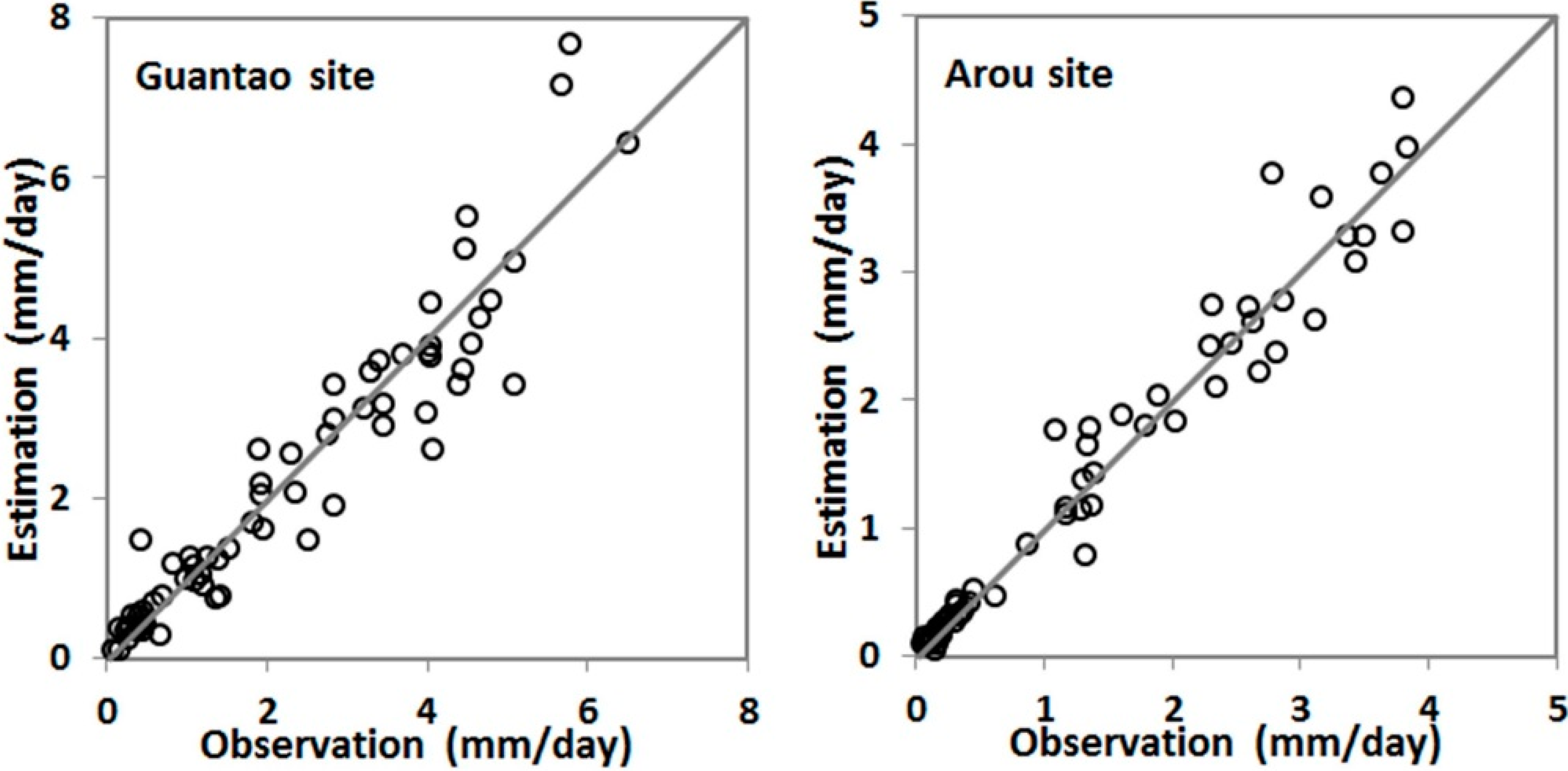
 Figure 4. Figure 4 shows that the ET estimates from the optimum method were close to observational values.
Figure 4. The comparisons of clear-sky ET estimates from the optimum method with in situ observations.
Remotesensing 07 03400 g004
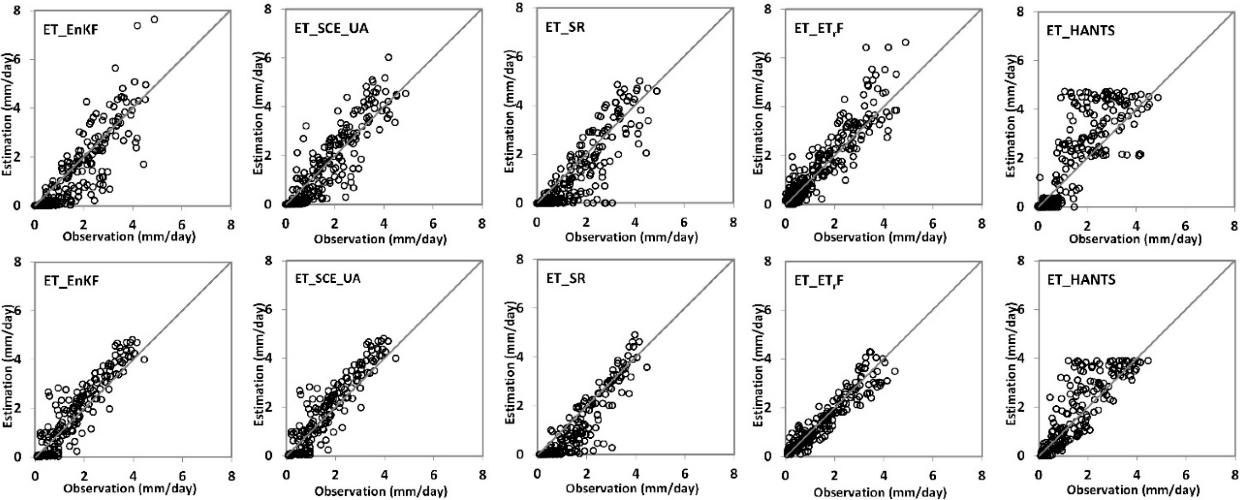
The continuous daily ET was reconstructed with discrete accumulated clear-sky daily ET values measured by EC instruments at the Guantao and Arou sites. The cloudy-day ET temporal reconstruction results from the developed data assimilation methods (ET_EnKF and ET_SCE_UA), ET_SR, ET_ETrF, and ET_HANTS method, were compared with the ET observations (see Figure 5). As shown, the data assimilation methods and the ET_ETrF method performed the best, as indicated by the scattering about the 1:1 line. The ET_SR method underestimated the cloudy-day ET significantly, and the ET_HANTS method overestimated.
Figure 5. The comparisons of cloudy-day ET between the model estimations and observations. (Guantao site result (top); Arou site result (bottom)).
Remotesensing 07 03400 g005
The statistics of each temporal reconstruction method are shown in Table 5. Over the whole time period, the RMSEs of most of the temporal reconstruction approaches were within 1.0 mm/day, except for the ET_HANTS method at the Guantao site (1.06 mm/day). The ET_ETrF method produced the lowest RMSE values, which were 0.61 and 0.37 mm/day at Guantao and Arou, respectively. MRE values of ET_SCE_UA method were around zero (−5.4% and −2.6% at the Guantao and Arou sites), indicating the lowest ET estimation bias. Of the two data assimilation methods, the ET_SCE_UA approach outperformed the ET_EnKF. As indicated in Section 2.3.1, the ET_SCE_UA approach can make full use of four neighbored clear-sky ET observations to update the model parameters, while the ET_EnKF method only uses one previous ET observations. Thus, the ET_SCE_UA approach can produce lower errors than ET_EnKF method. The performances of these methods were also analyzed during periods of vegetation growth and dormant vegetation, as shown in Table 5. The periods of vegetation growth usually had larger RMSEs than periods of vegetation dormancy, and over the entire period, because the ET value was larger in summer than the other seasons, which was caused by higher solar radiation. The MRE values of most methods were closer to zero during periods of vegetation growth than periods of dormant vegetation, except for the ET_HANTS method. The data assimilation, ET_SR, and ET_ETrF methods were all based on Penman-Monteith equation. Since the key parameter (surface resistance) of the Penman-Monteith equation is parameterized by leaf area index, it may get more accurate results for periods of vegetation growth than periods of vegetation dormancy [25].
Table 5. The statistics of temporal reconstruction approaches at the Guantao and Arou sites.
SiteSeasonStatisticsET_EnKFET_SCE_UAET_SRET_ETrFET_HANTS
GuantaoVegetation, growingMRE (%)−7.4−0.2−13.89.641.1
RMSE (mm/day)1.140.811.200.801.53
R (-)0.750.840.730.830.40
Vegetation, dormantMRE (%)−53.8−22.4−56.114.0−28.0
RMSE (mm/day)0.430.510.440.410.44
R (-)0.850.790.850.820.84
OverallMRE (%)−18.3−5.4−23.610.724.9
RMSE (mm/day)0.810.660.850.611.06
R (-)0.870.910.850.910.83
ArouVegetation, growingMRE (%)12.70.0−19.7−6.521.5
RMSE (mm/day)0.600.480.800.450.98
R (-)0.900.940.880.900.59
Vegetation, dormantMRE (%)−3.2−31.8−73.5−19.1−39.2
RMSE (mm/day)0.510.330.520.300.30
R (-)0.570.630.510.680.76
OverallMRE (%)9.6−2.6−25.410.512.9
RMSE (mm/day)0.570.410.660.370.73
R (-)0.930.960.910.950.88
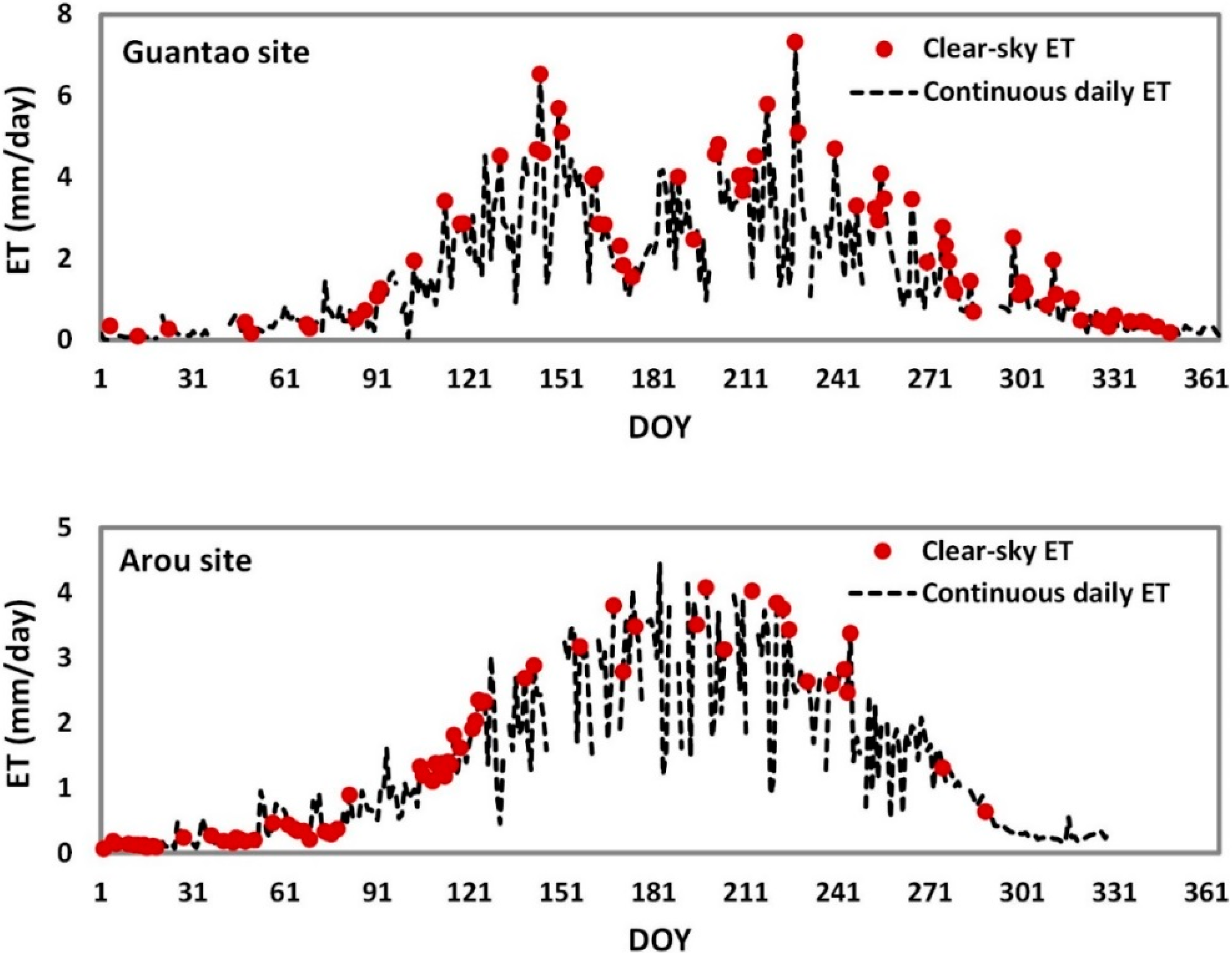
No soil moisture or precipitation data were used in any of the temporal reconstruction approaches. However, soil moisture may increase suddenly due to precipitation and thermal remote sensing is not able to detect this change during rainy days. The variations of soil moisture will lead to change in ET distributions. Thus, errors may be cut down by developing ET temporal reconstruction methods that can assimilate microwave soil moisture (e.g., SMAP), or precipitation observations. For the ET_HANTS method, the cloudy-sky ET can be estimated based on clear-sky ET observations. However, the clear-sky ET is usually higher than cloudy-sky ET, which is a result of larger values of solar radiation. Without an input for forcing data (e.g., solar radiation, precipitation), the ET_HANTS method cannot detect a sudden decrease in ET caused by clouds. Thus, the estimated cloudy-sky ET from ET_HANTS is usually larger than in situ measurements, as was found here and is indicated by Figure 5. Moreover, the ET_HANTS method produced smooth seasonal variation of cloudy-sky daily ET. Thus, the scattering from the ET_HANTS method was sparser than the others (see Figure 5). The surface resistance in the ET_SR method with cloudy-sky conditions was obtained with the clear-sky values and ancillary parameters (LAI, m(Tmin) and m(VPD) functions). Because threshold values of m(Tmin) and m(VPD) were constructed based on vegetation types globally [25], they may not suitable for all specific land cover and climatic condition and should be calibrated with local observations.
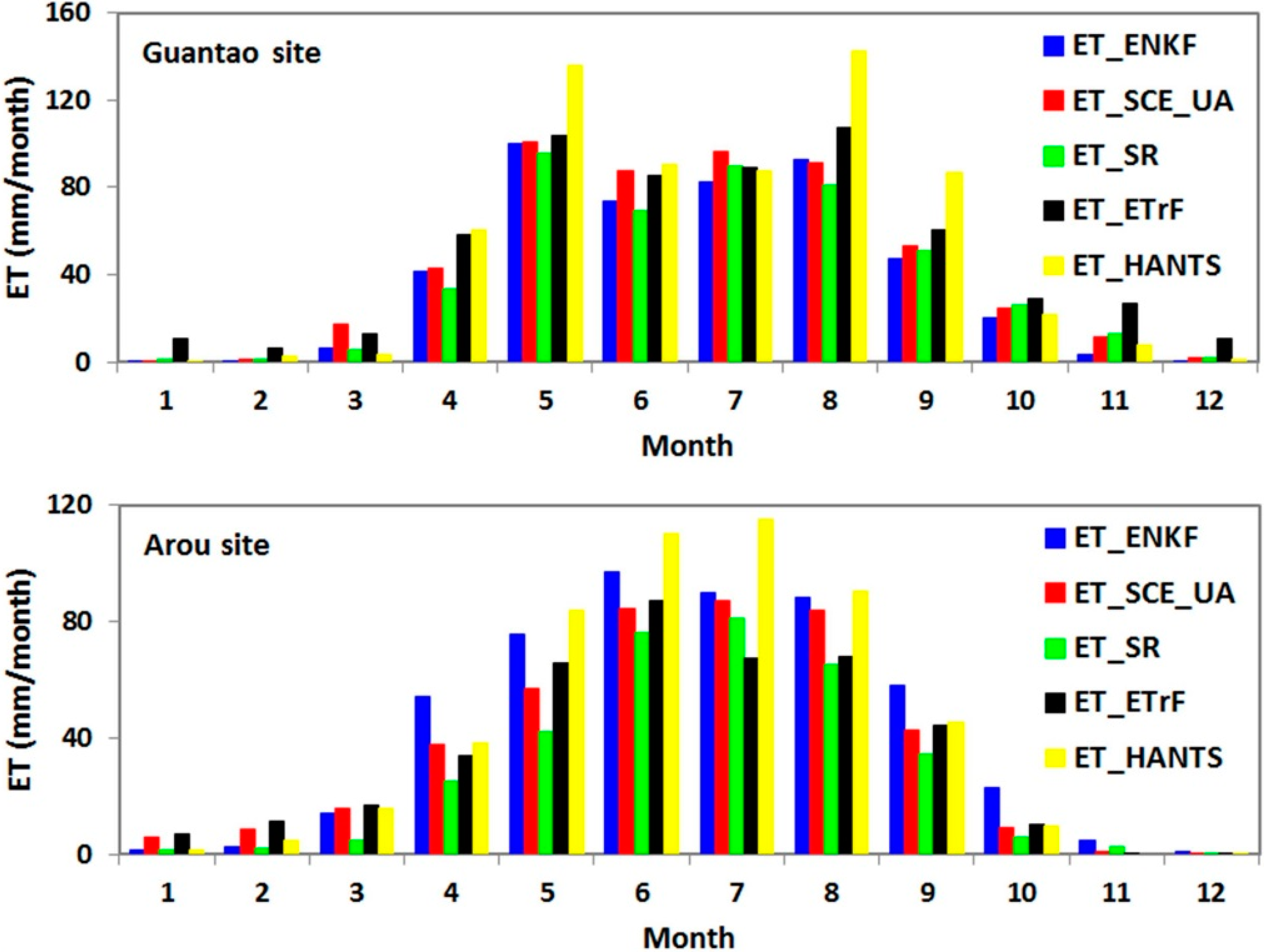
Figure 6. The monthly ET variations from five temporal reconstruction approaches.
Remotesensing 07 03400 g006
The monthly variation of ET at the Guantao and Arou sites is shown in Figure 6. From Figure 6, the five methods show similar trends. At the Guantao site, all the methods display dual-peak ET values, caused by different growth patterns of winter wheat and summer corn. The low ebb of the ET estimates is indicative of a crop rotation period, where the winter wheat was cut down and the summer corn was at the early stages of growth. The ET_HANTS method estimated an ET that was larger than the other methods for May and August, which are the months of peak ET for both winter wheat and summer corn. The ET_HANTS overestimated the ET by 24.9% (see Table 5), which was caused by the large error for these two months at the Guantao site. At the Arou site, all methods depict a single-peak ET trend throughout the year. The ET_HANTS overestimated the ET by 12.9%, which was caused by the large error from May to August.

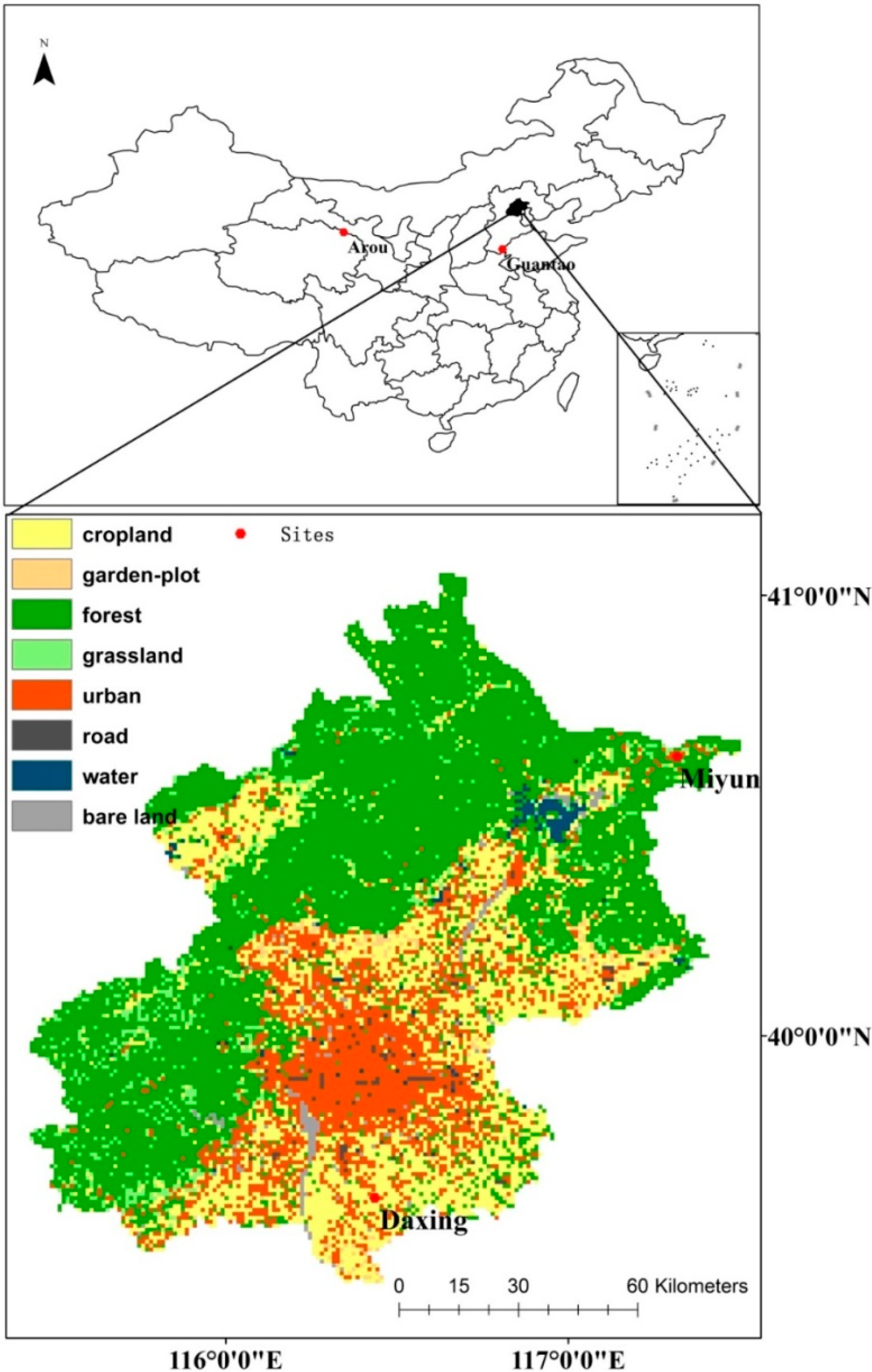
4.2. Regional Application

In this study, the regional instantaneous clear-sky ET values were estimated by the remotely sensed ET model proposed by Liu et al. [5]. The instantaneous ET estimates were upscaled to daily values with the combination of the SolRad and ConETrF methods (the “optimum method”). The ConEF method was also applied for comparison. Over land surface covered with vegetation (cropland, garden-plot, forest, and grassland in Figure 2), the SolRad and ConETrF methods were used for ET upscaling, during periods of vegetation dormancy and growth, respectively. Over land surface without vegetation (urban, water, road, and bare land), the SolRad method was used for ET upscaling over the entire year. In Beijing, the season of vegetation growth is from day of year (DOY) 100–283, for garden-plot, forest, and grassland areas, but for cropland, the season of vegetation growth is from DOY 100–161 and 182–283, according to vegetation phenology. As discussed in Section 4.1, the ET_ETrF and ET_SCE_UA methods performed the best out of the ET temporal reconstruction approaches. Thus, those approaches were selected to produce the continuous daily ET with upscaled clear-sky daily ET for the Beijing area. The ET_SR method was also applied in Beijing for comparison. The comparisons between model estimates and the LAS observations are shown in Figure 7 and Figure 8.
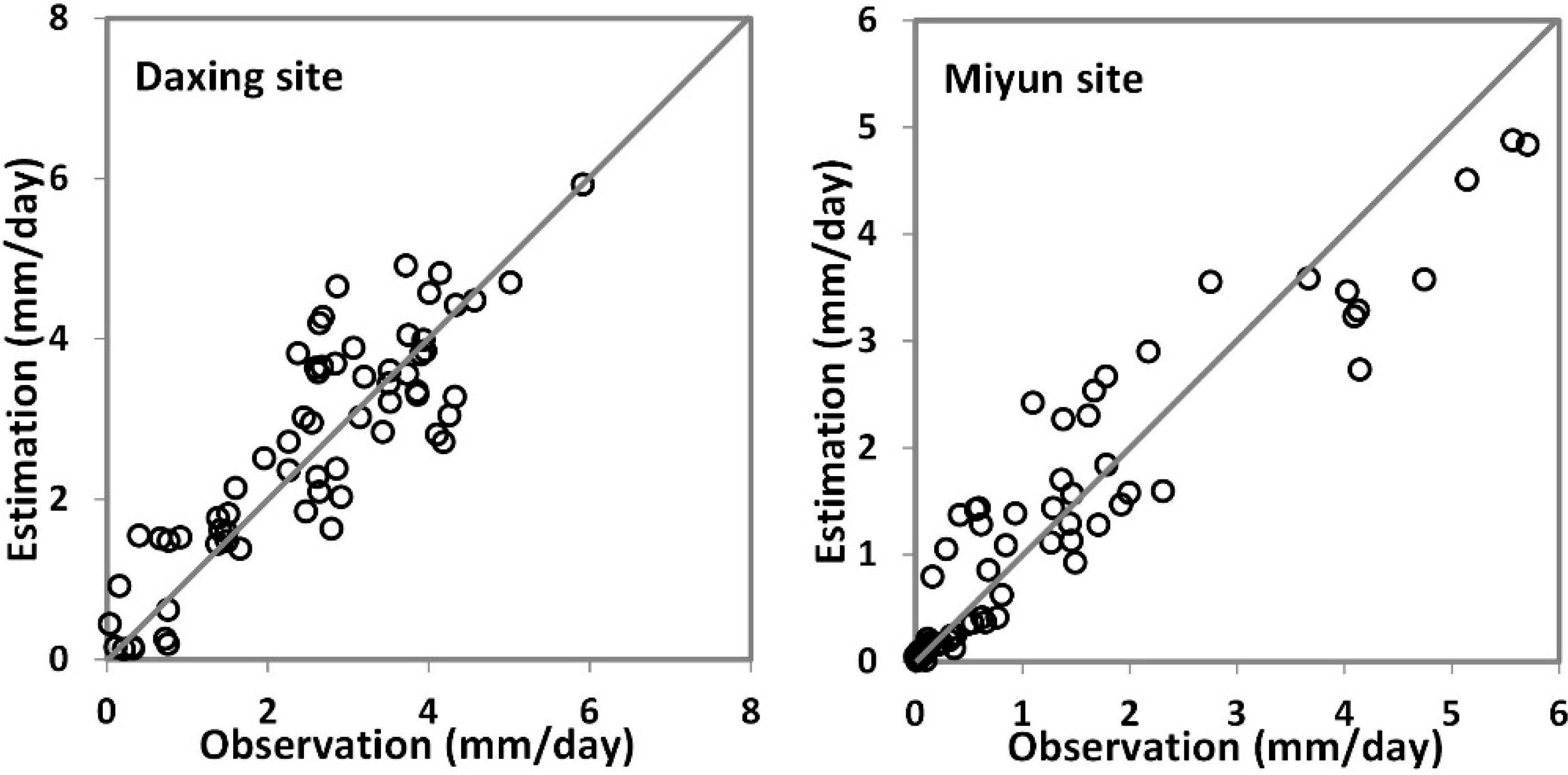
Figure 7 shows the temporal upscaling results of the instantaneous ET estimates with the optimum method. The model estimates were close to LAS daily ET observations and the scatter plots approximately form 1:1 lines. At the Daxing site, the MRE (RMSE) value was 5.4% (0.72 mm/day). The corresponding MRE (RMSE) for the Miyun site was 0.3% (0.54 mm/day). Thus, the optimum method showed minor bias and low RMSE values at the two sites, which indicates that the optimum method is a suitable thermal ET upscaling method.
Figure 7. The comparisons of clear-sky daily ET estimates from the optimum method with LAS observations.
Remotesensing 07 03400 g007
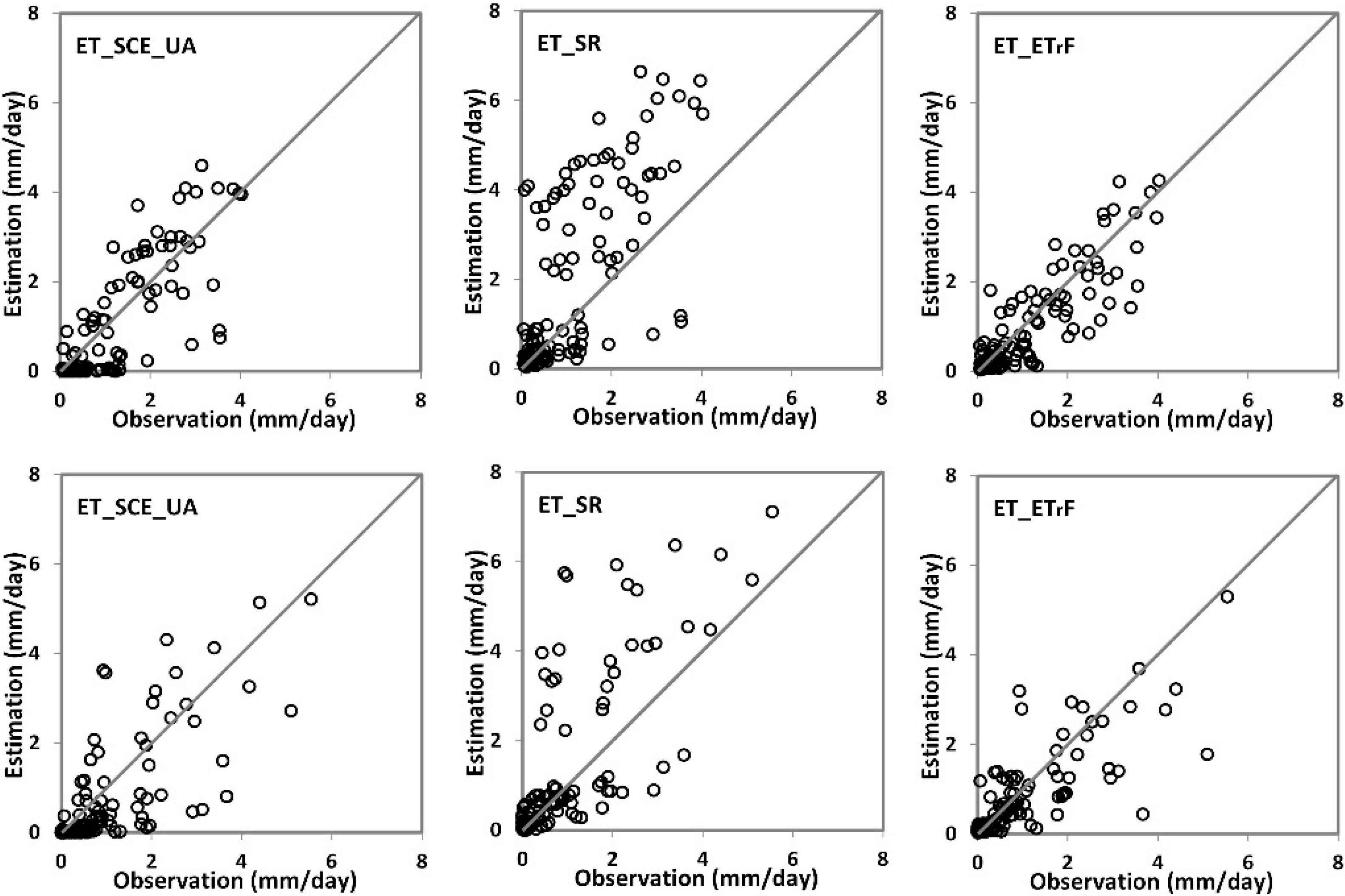
The continuous daily ET was reconstructed based on the discrete clear-sky daily ET upscaling results. The comparisons between reconstructed cloudy-day estimates and LAS observations are shown in Figure 8. Compared with observations, the scatter plots from the ET_SCE_UA and ET_ETrF methods are close to 1:1 lines. The ET_SR method overestimated the continuous daily ET compared with observational values. The statistics of the temporal reconstruction approaches are summarized in Table 6. The ET_ETrF and ET_SCE_UA methods produced lower RMSEs and MREs, and showed higher correlations than the ET_SR method. The ET_ETrF method performed the best at both the Daxing and Miyun sites. At the Miyun site, the ET_ETrF method underestimated the continuous daily ET when the value was larger than 3 mm/day (Figure 8), which was caused by the underestimation of clear-sky ET, derived from the remotely sensed model and the upscaling method (Figure 7).
Figure 8. The comparisons of cloudy-day ET between model estimates and in situ observations. (Daxing site result (top row); Miyun site result (bottom row)).
Remotesensing 07 03400 g008
Table 6. The statistics of temporal reconstruction approaches at the Daxing and Miyun sites.
Site NameStatisticsET_SCE_UAET_ETrFET_SR
DaxingMRE (%)−14.43−12.9872.34
RMSE (mm/day)0.740.561.60
R (-)0.830.870.73
MiyunMRE (%)−23.98−16.2442.74
RMSE (mm/day)0.890.751.32
R (-)0.740.770.74
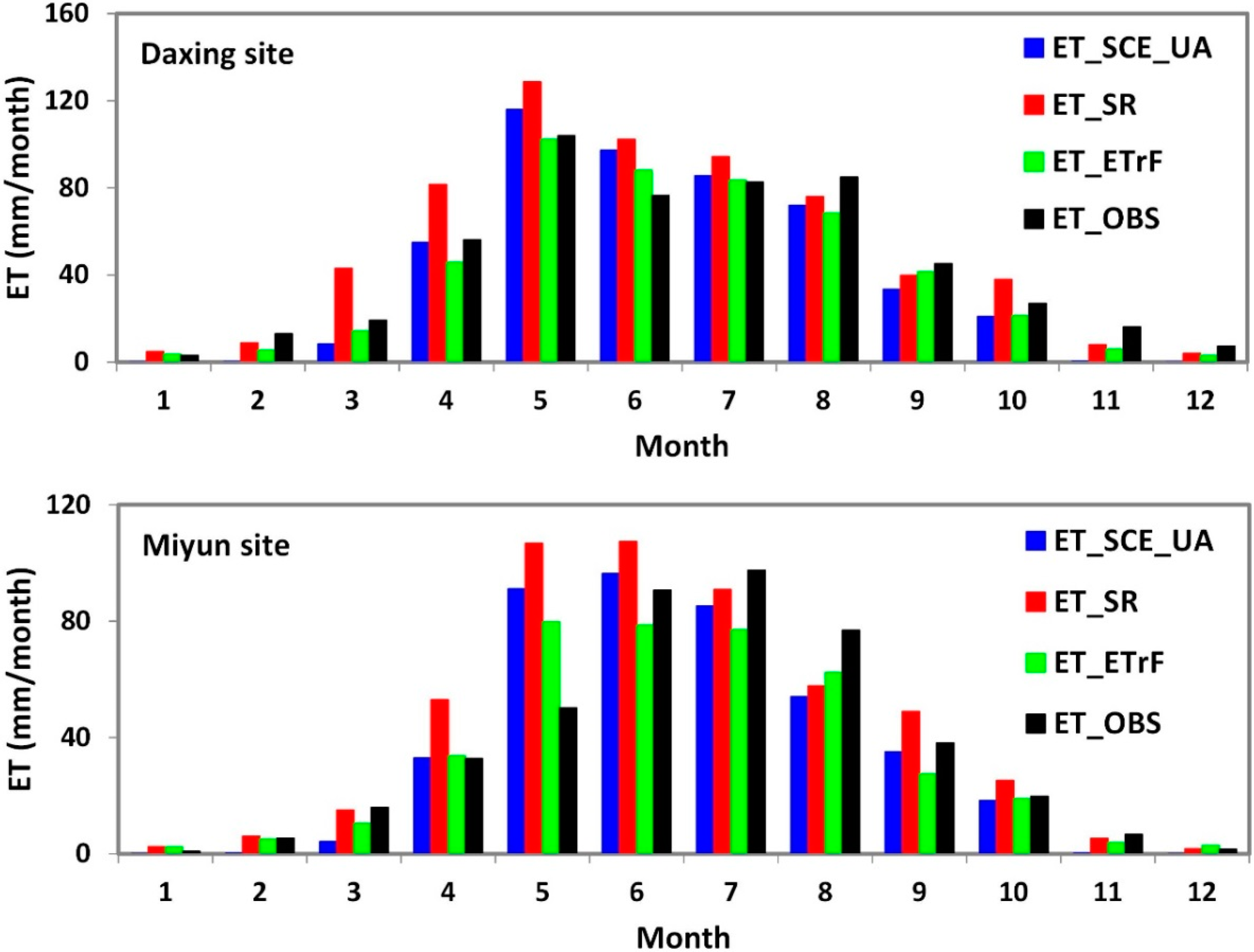
The comparisons of monthly accumulated ET estimates and LAS observations are shown in Figure 9. Results from the three methods had the same trends as the observations. The Daxing site exhibits weak dual-peak ET variation, and the Miyun site shows single-peak ET variation. At the Daxing site, ET estimates from the three methods were higher than the observations. At the Miyun site, ET estimates from the three methods were higher than the observations from Apr. to Jun., but lower than the observations in Aug. The ET_ETrF method had the lowest RMSE values (8.2 mm/month and 12.3 mm/month), and MRE values from ET_SCE_UA were closer to zero (−7.84% and −3.56%) at the Daxing and Miyun sites, respectively.
Figure 9. The comparisons of monthly ET between model estimates and observations at the Daxing and Miyun sites.
Remotesensing 07 03400 g009
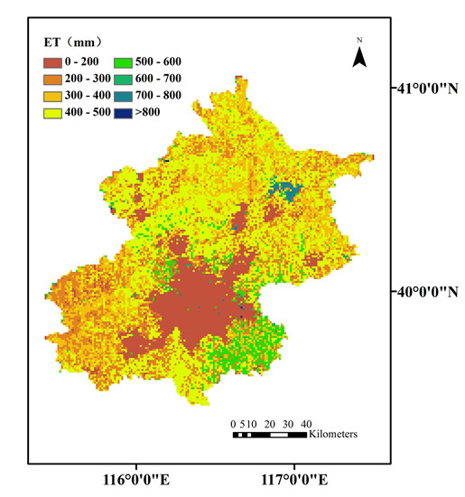
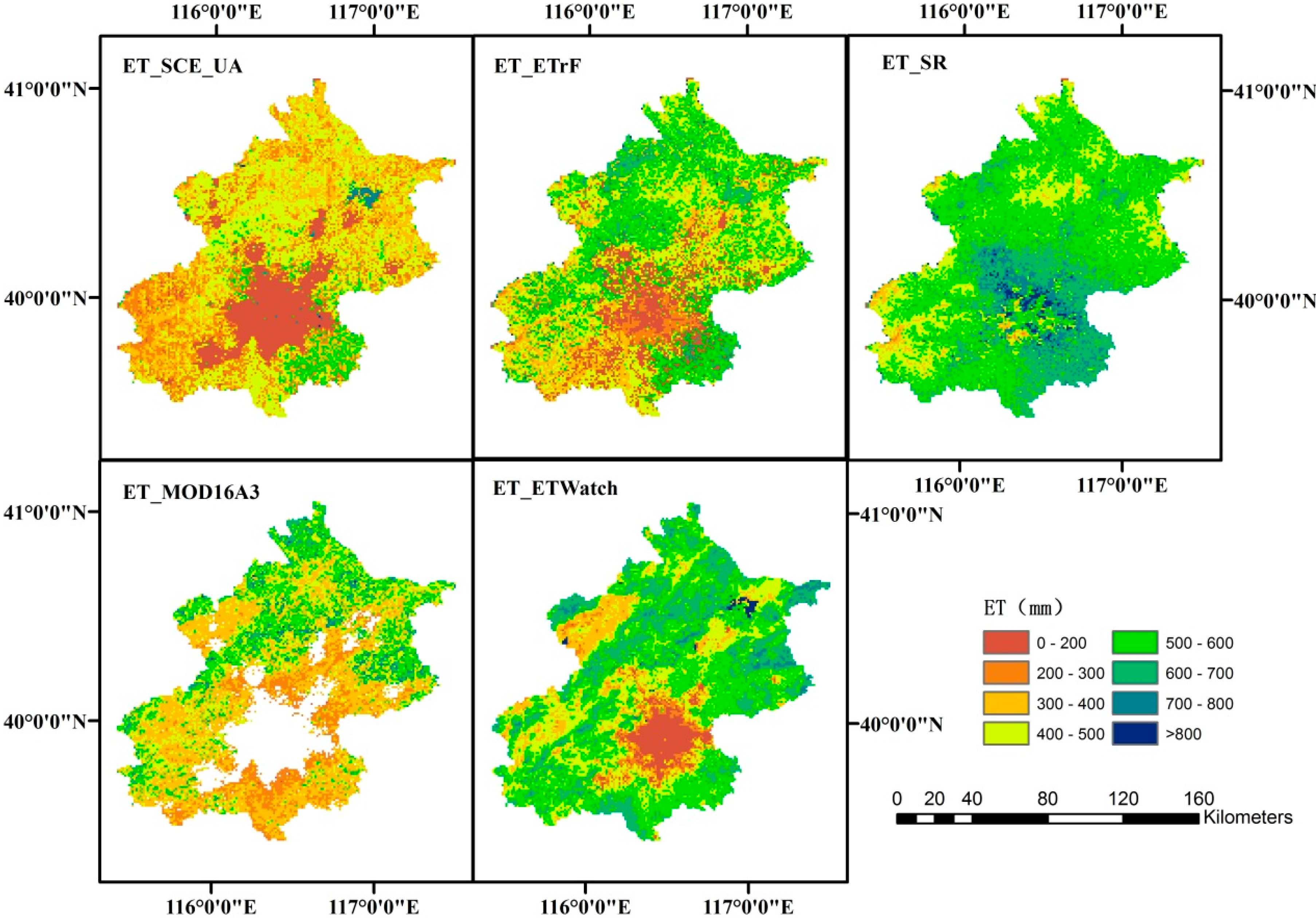
The regional annual ET estimates from the three methods are shown in Figure 10, and the ET products from MOD16A3 and ETWatch are also shown, for comparison. Over the whole region, the estimations from the ET_ETrF and ET_SCE_UA methods had the same trend as the ET products from ETWatch. In the downtown area of Beijing, ET values were smaller than in other areas, as expected, due to paved land surfaces. The cropland and forest distributed around the downtown area showed high annual ET values, caused by irrigation and vegetation transpiration. The largest annual ET values were found over open water in the Miyun reservoir area, north of Beijing. However, the ET_SR method performed poorly over some of the urban areas, which showed large ET values. The ET_SR method is also adopted by MOD16A3, but no values were obtained from urban and water areas over Beijing.
The annual ET values of different land cover types are shown in Table 7. The ET values over water, cropland, garden-plot, forest, and grassland were in the first class with larger ET from the ET_SCE_UA, ET_ETrF, MOD16A3, and ETWatch methods. Over the water area, most of the available energy is evaporated to water vapor that leads to largest ET estimates. Irrigation of vegetated lands, e.g., croplands and garden-plots, made vegetation transpiration values much larger than values from other vegetated lands that were unirrigated, e.g., unirrigated grassland. Forested land is generally located in mountainous regions, which experience high levels of precipitation, but a large portion of the rainfall becomes runoff and does not add to ET. Thus, forested land tends to have less soil water, and lower ET values than cropland and garden-plot. The smallest ET values were found in the urban areas of Beijing, because most of the land is paved, not vegetated, and precipitation is routed as storm water into the city’s sewer system. Since the Penman-Monteith method is better suited for use with densely vegetated land cover, the ET_SR method did not perform well over urban areas. The corresponding values for the ET_SCE_UA, ET_ETrF, ET_SR, and ETWatch methods were 347 mm, 356 mm, 580 mm, and 470 mm, respectively. The results from the ET_ETrF and ET_SCE_UA methods were closer to the water balance derived value (387 mm), and the ET_SR and ETWatch methods had larger errors. Thus, annual ET from the ET_SCE_UA method was in the same order of magnitude as the water balance method, and ET estimates of different land covers were more reasonable than the ET_ETrF method (ET from forest was larger than water).
Figure 10. Annual ET distributions for the Beijing area in 2009.
Remotesensing 07 03400 g010
Table 7. Annual ET over different land covers in 2009.
Land Cover TypeET_SCE_UAET_ETrFET_SRMOD16A3ETWatch
cropland405446604295483
garden plot404463626290505
forest334488534428549
grassland362338499390529
urban153146609-382
road94120504-340
water705480656-522
bare land320368608207447
The averaged ET values over vegetated land covers (cropland, garden-plot, forest and grassland) were 376 mm, 434 mm, 566 mm, 350 mm, and 516 mm for ET_SCE_UA, ET_ETrF, ET_SR, MOD16A3, and ETWatch, respectively. ET estimates were the highest from the ET_SR and ETWatch, while ET from MOD16A3 was the smallest, which indicates that ET was underestimated over the Beijing area. Moreover, ET values from forest and grassland were larger than the values from cropland and garden-plots, which did not seem reasonable for MOD16A3 ET products.

5. Conclusions

Long-term regional evapotranspiration is important for water resources planning and management and water-saving agricultural. The development of remotely sensed ET models enabled the mapping of regional ET at the time of satellite overpass. However, thermal remote sensing data are often contaminated by clouds. Thus, temporal upscaling methods are needed to upscale the instantaneous ET into daily values. Moreover, continuous daily ET should be reconstructed with discrete clear-sky ET. In this study, five temporal upscaling methods were selected to extend the instantaneous ET to daily values, and five temporal reconstruction approaches were used to generate continuous daily ET values for one year. These methods were compared extensively at two sites in China, namely, Guantao and Arou, which were selected based on distinct climate conditions. For regional application, annual ET distributions over the Beijing area for 2009 were produced with these methods, and the total annual ET was compared with the water balance method. Additionally, ET products from MOD16A3 and ETWatch were obtained for regional comparisons. LAS observations from two sites within Beijing (Daxing and Miyun) were acquired for ET estimate validations.
The five temporal upscaling methods were compared with EC measurements at the Guantao and Arou sites. Comparisons showed that the SolRad and ConETrF methods performed the best, as indicated by having produced the smallest RMSE values. The commonly used ConEF method underestimated the daily ET, due to the increasing EF in the early morning and late afternoon. The CorEF and DiEF methods attempted to correct the underestimation by adding 10% of the ET, and by using three factors that enhance daily ET estimation with instantaneous EF observation. Because reference ET can capture impacts from changes in wind and humidity, the ConETrF method was more stable than the ConEF and its related methods (CorEF and DiEF methods). Moreover, the ConETrF method produced the smallest RMSE values during the season of vegetation growth, where Penman-Monteith equation performs well. The SolRad method performed best during the season of vegetation dormancy, and for non-vegetated land cover. The combination of the SolRad and ConETrF methods, each optimized with respect to land cover and time period, produced RMSE values of 0.58 mm/day and 0.25 mm/day, at the Guantao and Arou sites, respectively. The corresponding MRE values were −3.7% and 0%. Thus, the combination of the SolRad and ConETrF methods (the “optimum method”) performed the best overall.
The five temporal reconstruction approaches were used to generate continuous daily ET values with discrete clear-sky daily ET at the Guantao and Arou sites. Through comparison, the reference evapotranspiration method (ET_ETrF), and the data assimilation method of the SCE_UA algorithm (ET_SCE_UA), were found to perform the best at the two sites. The ET_ETrF method produced the lowest RMSE values of 0.61 and 0.37 mm/day at Guantao and Arou, respectively. The MRE values of the ET_SCE_UA method were around zero (−5.4% and −2.6% at the Guantao and Arou sites), which turned out to be the lowest ET estimation biases. The surface resistance method (ET_SR) and the HANTS method (ET_HANTS) had large errors compared to observational values. The temporal reconstructed continuous daily ET values might have had larger errors than monthly ET values, because the random errors of continuous daily ET values cancelled each other out. Rainfall that occurred during cloudy-days increased the soil moisture, EF and ETrF, which may have led to errors in reconstructing continuous daily ET with discrete clear-sky ET values. In future studies, soil moisture information should be included to mitigate the variations of wet land surface conditions.
For regional application, a remotely sensed ET model was selected to calculate the instantaneous regional ET based on MODIS data. The optimum method was used to upscale the instantaneous ET to daily values. The ET_SCE_UA and ET_ETrF methods were used to reconstruct continuous daily ET based on clear-sky daily ET. The distribution of calculated annual ET over the Beijing area had a similar trend to the MOD16A3 and ETWatch products. In 2009, the annual ET values over the Beijing area for the ET_SCE_UA, ET_ETrF, ET_SR, and ETWatch methods were 347 mm, 356 mm, 580 mm, and 470 mm, respectively. The results from the ET_ETrF and ET_SCE_UA methods were closer to the water balance derived annual ET for Beijing (387 mm). The ET estimates from ET_SCE_UA were more reasonable than those from ET_ETrF over different land covers.
Although ET temporal upscaling and reconstruction methods have been compared at two typical sites and applied over the Beijing area in China, they need to be validated over broader flux sites around the world to assess broader application.

Acknowledgments

We thank the editors and four anonymous reviewers very much for their valuable comments that greatly improved the presentation of this paper. This research was jointly supported by the National Natural Science Foundation of China (91125002 and 41201330), the High-Tech Research and Development Program of China (No. 2013AA12A301), and the Fundamental Research Funds for the Central Universities (2012LYB37).

Author Contributions

Tongren Xu and Shaomin Liu prepared the manuscript. Lu Xu and Yujie Chen ran the models. Zhenzhen Jia contributed to the discussion. Ziwei Xu collected and processed the data. Jeffrey Nielson improved the English expression of the manuscript.

Conflicts of Interest

The authors declare no conflict of interest.

References

  1. Baldocchi, D.; Falge, E.; Gu, L.H.; Olson, R.; Hollinger, D.; Running, S.; Anthoni, P.; Bernhofer, C.; Davis, K.; Evans, R.; et al. FLUXNET: A new tool to study the temporal and spatial variability of ecosystem–scale carbon dioxide, water vapor, and energy flux densities. Bull. Amer. Meteorol. Soc. 2001, 82, 2415–2434. [Google Scholar]
  2. Li, X.; Cheng, G.D.; Liu, S.M.; Xiao, Q.; Ma, M.G.; Jin, R.; Che, T.; Liu, Q.H.; Wang, W.Z.; Qi, Y.; et al. Heihe watershed allied telemetry experimental research (HiWATER): Scientific objectives and experimental design. Bull. Amer. Meteorol. Soc. 2013, 94, 1145–1160. [Google Scholar] [CrossRef]
  3. Cheng, G.D.; Li, X.; Zhao, W.Z.; Xu, Z.M.; Feng, Q.; Xiao, S.C.; Xiao, H.L. Integrated study of the water–ecosystem–economy in the Heihe River Basin. Natl. Sci. Rev. 2014, 1, 413–428. [Google Scholar] [CrossRef]
  4. Su, Z. The surface energy balance system (SEBS) for estimation of turbulent heat fluxes. Hydrol. Earth Syst. Sc. 2002, 6, 85–99. [Google Scholar] [CrossRef]
  5. Liu, S.M.; Hu, G.; Lu, L.; Mao, D. Estimation of regional evapotranspiration by TM/ETM+ data over heterogeneous surfaces. Photogramm. Eng. Rem. Sens. 2007, 73, 1169–1178. [Google Scholar] [CrossRef]
  6. Tang, R.; Li, Z.L.; Tang, B. An application of the Ts-VI triangle method with enhanced edges determination for evapotranspiration estimation from modis data in arid and semi-arid regions: Implementation and validation. Remote Sens. Environ. 2010, 114, 540–551. [Google Scholar] [CrossRef]
  7. Yao, Y.J.; Liang, S.; Li, X.; Hong, Y.; Fisher, J.B.; Zhang, N.N.; Chen, J.; Cheng, J.; Zhao, S.; Zhang, X.; et al. Bayesian multimodel estimation of global terrestrial latent heat flux from eddy covariance, meteorological, and satellite observations. J. Geophys. Res. 2014, 119, 4521–4545. [Google Scholar] [CrossRef]
  8. Long, D.; Singh, V.P. A two-source trapezoid model for evapotranspiration from satellite imagery. Remote Sens. Environ. 2012, 121, 370–388. [Google Scholar] [CrossRef]
  9. Yang, Y.; Shang, S.H. A hybrid dual-source scheme and trapezoid framework-based evapotranspiration model (HTEM) using satellite images: Algorithm and model test. J. Geophys. Res. 2013, 118, 2284–2300. [Google Scholar] [CrossRef]
  10. Yang, Y.; Long, D.; Shang, S. Remote estimation of terrestrial evapotranspiration without using meteorological data. Geophys. Res. Lett. 2013, 40, 3026–3030. [Google Scholar] [CrossRef]
  11. Merlin, O.; Chirouze, J.; Olioso, A.; Jarlan, L.; Chehbouni, A.; Boulet, G. An image-based four-source surface energy balance model to estimate crop evapotranspiration from solar reflectance /thermal emission data (SEB-4S). Agric. For. Meteorol. 2014, 184, 188–203. [Google Scholar] [CrossRef] [Green Version]
  12. Shuttlewroth, W.J.; Gurney, R.J.; Hsu, A.Y.; Ormsby, J.P. FIFE: The variation in energy partition at surface flux sites. Remote Sens. Large-Scale Glob. Process. 1989, 186, 67–74. [Google Scholar]
  13. Sugita, M.; Brutsaert, W. Daily evaporation over a region from lower boundary layer profiles measured with radiosondes. Water Resour. Res. 1991, 27, 747–752. [Google Scholar] [CrossRef]
  14. Brutsaert, W.; Sugita, M. Application of self-preservation in the diurnal evolution of the surface energy budget to determine daily evaporation. J. Geophys. Res. 1992, 97, 18377–18382. [Google Scholar] [CrossRef]
  15. Gentine, P.; Entekhabi, D.; Chehbouni, A.; Boulet, G.; Duchemin, B. Analysis of evaporative fraction diurnal behavior. Agric. For. Meteorol. 2007, 143, 13–29. [Google Scholar] [CrossRef] [Green Version]
  16. Anderson, M.C.; Norman, J.M.; Diak, G.R.; Kustas, W.P.; Mecikalski, J.R. A two-source time-integrated model for estimating surface fluxes using thermal infrared remote sensing. Remote Sens. Environ. 1997, 60, 195–216. [Google Scholar] [CrossRef]
  17. Van Niel, T.G.; McVicar, T.R.; Roderick, M.L.; van Dijk, A.I.J.M.; Renzullo, L.J.; van Gorsel, E. Correcting for systematic error in satellite-derived latent heat flux due to assumptions in temporal scaling: Assessment from flux tower observations. J. Hydrol. 2011, 409, 140–148. [Google Scholar] [CrossRef]
  18. Jackson, R.D.; Hatfield, J.L.; Reginato, R.J.; Idso, S.B.; Pinter, P.J. Estimation of daily evapotranspiration from one time-of-day measurements. Agric. Water Manage. 1983, 7, 351–362. [Google Scholar]
  19. Ryu, Y.; Baldocchi, D.D.; Black, T.A.; Detto, M.; Law, B.E.; Leuning, R.; Miyata, A.; Reichstein, M.; Vargas, R.; Ammann, C.; et al. On the temporal upscaling of evapotranspiration from instantaneous remote sensing measurements to 8-day mean daily-sums. Agric. For. Meteorol. 2012, 152, 212–222. [Google Scholar] [CrossRef] [Green Version]
  20. Trezza, R. Evapotranspiration Using A Satellite-Based Surface Energy Balance with Standardized Ground Control. Ph.D. Thesis, Utah State University, Logan, UT, USA, 2002. [Google Scholar]
  21. Delogu, E.; Boulet, G.; Olioso, A.; Coudert, B.; Chirouze, J.; Ceschia, E.; le Dantec, V.; Marloie, O.; Chehbouni, G.; Lagouarde, J.P. Reconstruction of temporal variations of evapotranspiration using instantaneous estimates at the time of satellite overpass. Hydrol. Earth Syst. Sci. 2012, 16, 2995–3010. [Google Scholar] [CrossRef] [Green Version]
  22. Colaizzi, P.D.; Evett, S.R.; Howell, T.A.; Tolk, J.A. Comparison of five models to scale daily evapotranspiration from one-time-of-day measurements. Trans. ASABE 2006, 49, 1409–1417. [Google Scholar] [CrossRef]
  23. Tang, R.L.; Li, Z.L.; Sun, X.M. Temporal upscaling of instantaneous evapotranspiration: An intercomparison of four methods using eddy covariance measurements and MODIS data. Remote Sens. Environ. 2013, 138, 102–118. [Google Scholar] [CrossRef]
  24. Cammalleri, C.; Anderson, M.C.; Kustas, W.P. Upscaling of evapotranspiration fluxes from instantaneous to daytime scales for thermal remote sensing applications. Hydrol. Earth Syst. Sci. 2014, 18, 1885–1894. [Google Scholar] [CrossRef] [Green Version]
  25. Mu, Q.; Heinsch, F.A.; Zhao, M.; Running, S.W. Development of a global evapotranspiration algorithm based on MODIS and global meteorology data. Remote Sens. Environ. 2007, 111, 519–536. [Google Scholar] [CrossRef]
  26. Mu, Q.Z.; Zhao, M.S.; Running, S.W. Improvements to a MODIS global terrestrial evapotranspiration algorithm. Remote Sens. Environ. 2011, 115, 1781–1800. [Google Scholar] [CrossRef]
  27. Wu, B.F.; Yan, N.N.; Xiong, J.; Bastiaanssen, W.G.M.; Zhu, W.W.; Stein, A. Validation of ETWatch using field measurements at diverse landscapes: A case study in Hai Basin of China. J. Hydrol. 2012, 436, 67–80. [Google Scholar] [CrossRef]
  28. Allen, R.G.; Tasumi, M.; Trezza, R. Satellite-based energy balance for mapping evapotranspiration with internalized calibration (METRIC)-Model. J. Irrig. Drain. Eng. 2007, 133, 380–394. [Google Scholar] [CrossRef]
  29. Teixeira, A.H.D.C.; Bastiaanssen, W.G.M.; Ahmad, M.D.; Bos, M.G. Reviewing SEBAL input parameters for assessing evapotranspiration and water productivity for the Low-Middle Sao Francisco River basin, Brazil Part B: Application to the regional scale. Agric. For. Meteorol. 2009, 149, 477–490. [Google Scholar] [CrossRef]
  30. Verhoef, W. Application of Harmonic Analysis of NDVI Time Series (HANTS). In Fourier Analysis of Temporal NDVI in the Southern African and American Continents; Azzali, S., Menenti, M., Eds.; DLO Winand Staring Centre: Wageningen, The Netherlands, 1996; pp. 19–24. [Google Scholar]
  31. Roerink, G.J.; Menenti, M.; Verhoef, W. Reconstructing cloudfree NDVI composites using Fourier analysis of time series. Int. J. Remote Sens. 2000, 21, 1911–1917. [Google Scholar] [CrossRef]
  32. Jia, L.; Xi, G.; Liu, S.; Huang, C.; Yan, Y.; Liu, G. Regional estimation of daily to annual regional evapotranspiration with MODIS data in the Yellow River Delta wetland. Hydrol. Earth Syst. Sci. 2007, 13, 1775–1787. [Google Scholar]
  33. Bennett, A.F. Inverse Methods in Physical Oceanography; Cambridge Univ. Press: New York, NY, USA, 1992. [Google Scholar]
  34. Reichle, R.H. Data assimilation methods in the Earth sciences. Adv. Water Resour. 2008, 31, 1411–1418. [Google Scholar] [CrossRef]
  35. Evensen, G. Sequential data assimilation with a nonlinear quasi-geostrophic model using Monte Carlo methods to forecast error statistics. J. Geophys. Res. 1994, 99, 10143–10162. [Google Scholar] [CrossRef]
  36. Duan, Q.Y.; Gupta, V.K.; Sorooshian, S. Shuffled complex evolution approach for effective and efficient global minimization. J. Optimiz. Theory App. 1993, 76, 501–521. [Google Scholar] [CrossRef]
  37. Han, X.; Li, X. An evaluation of the nonlinear/non-Gaussian filters for the sequential data assimilation. Remote Sens. Environ. 2008, 112, 1434–1449. [Google Scholar] [CrossRef]
  38. Reichle, R.H.; McLaughlin, D.B.; Entekhabi, D. Variational data assimilation of microwave radiobrightness observations for land surface hydrology applications. IEEE Trans. Geosci. Remote Sens. 2001, 39, 1708–1718. [Google Scholar] [CrossRef]
  39. Reichle, H.R.; Mclaughlin, D.B.; Entekhabi, D. Hydrologic data assimilation with the ensemble Kalman filter. Mon. Wea. Rev. 2002, 130, 103–114. [Google Scholar] [CrossRef]
  40. Huang, C.L.; Li, X.; Lu, L. Retrieving soil temperature profile by assimilating MODIS LST products with ensemble Kalman filter. Remote Sens. Environ. 2008, 112, 1320–1336. [Google Scholar] [CrossRef]
  41. Bateni, S.M.; Liang, S. Estimating surface energy fluxes using a dual-source data assimilation approach adjoined to the heat diffusion equation. J. Geophys. Res. 2012, 117, D17118. [Google Scholar]
  42. Xu, T.R.; Liu, S.M.; Liang, S.L.; Qin, J. Improving predictions of water and heat fluxes by assimilating MODIS land surface temperature products into the common land model. J. Hydrometeorol. 2011, 12, 227–244. [Google Scholar] [CrossRef]
  43. Xu, T.R.; Liang, S.L.; Liu, S.M. Estimating turbulent fluxes through assimilation of geostationary operational environmental satellites data using ensemble Kalman filter. J. Geophys. Res. 2011, 116, D09109. [Google Scholar]
  44. Xu, T.R.; Bateni, S.M.; Liang, S.; Entekhabi, D.; Mao, K.B. Estimation of surface turbulent heat fluxes via variational assimilation of sequences of land surface temperatures from Geostationary Operational Environmental Satellites. J. Geophys. Res. 2014, 119, 10780–10798. [Google Scholar]
  45. Gu, J.; Li, X.; Huang, C.L.; Okin, G.S. A simplified data assimilation method for reconstructing time-series MODIS NDVI data. Adv. Space Res. 2009, 44, 501–509. [Google Scholar] [CrossRef]
  46. Xiao, Z.Q.; Liang, S.; Wang, J.D.; Chen, P.; Yin, X.J.; Zhang, L.Q.; Song, J.L. Use of general regression neural networks for generating the GLASS leaf area index product from time-series MODIS surface reflectance. IEEE Trans. Geosci. Remote Sens. 2014, 52, 209–223. [Google Scholar] [CrossRef]
  47. Alavi, N.; Warland, J.S.; Berg, A.A. Filling gaps in evapotranspiration measurements for water budget studies: Evaluation of a Kalman filtering approach. Agric. For. Meteorol. 2009, 141, 57–66. [Google Scholar] [CrossRef]
  48. Allen, R.G.; Pereira, L.S.; Raes, D. Crop Evapotranspiration (Guidelines For Computing Crop Water Requirements). FAO Irrigation and Drainage Paper No. 56. Available online: http://www.fao.org/docrep/X0490E/X0490E00.htm (accessed on 20 March 2015).
  49. Saltelli, A.; Bolado, R. An alternative way to compute Fourier amplitude sensitivity test (FAST). Comput. Stat. Data Anal. 1999, 26, 445–460. [Google Scholar] [CrossRef]
  50. Liu, S.M.; Xu, Z.W.; Zhu, Z.L.; Jia, Z.Z.; Zhu, M.J. Measurements of evapotranspiration from eddy-covariance systems and large aperture scintillometers in the Hai River Basin, China. J. Hydrol. 2013, 487, 24–38. [Google Scholar] [CrossRef]
  51. Li, X.; Li, X.W.; Li, Z.Y.; Ma, M.G.; Wang, J.M.; Xiao, Q.; Liu, Q.; Che, C.; Chen, E.X.; Yan, G.J.; et al. Watershed allied telemetry experimental research. J. Geophys. Res. 2009. [Google Scholar] [CrossRef]
  52. Liu, S.M.; Xu, Z.W.; Wang, W.Z.; Jia, Z.Z.; Zhu, M.J.; Bai, J.; Wang, J.M. A comparison of eddy-covariance and large aperture scintillometer measurements with respect to the energy balance closure problem. Hydrol. Earth Syst. Sci. 2011, 15, 1291–1306. [Google Scholar] [CrossRef]
  53. Yang, K.; Wang, J. A temperature prediction-correction method for estimating surface soil heat flux from soil temperature and moisture data. Sci. China Ser. D. 2008, 51, 721–729. [Google Scholar] [CrossRef]
  54. McVicar, T.R.; van Niel, T.G.; Li, L.T.; Hutchinson, M.F.; Mu, X.M.; Liu, Z.H. Spatially distributing monthly reference evapotranspiration and pan evaporation considering topographic influences. J. Hydrol. 2007, 38, 196–220. [Google Scholar] [CrossRef]
  55. Jia, Z.Z.; Liu, S.M.; Xu, Z.W.; Chen, Y.J.; Zhu, M.J. Validation of remotely sensed evapotranspiration over the Hai River Basin, China. J. Geophys. Res. 2012, 117, D13113. [Google Scholar] [CrossRef]

