1. Introduction
The importance of floods as environmental drivers has long been recognised by many scientific disciplines (geomorphology, biology, ecology,
etc.). They entail different environmental and natural processes which provide connectivity between rivers and their floodplains, playing a key role in structuring vegetation communities and altering aquatic biota, developing floodplain habitats, forming channel morphologies, and replenishing aquifers and groundwater reservoirs within many different ecosystems [
1,
2,
3]. However, floods are also one of the most significant natural disasters which can cause severe economic and social losses [
4,
5,
6,
7,
8]. Predictive global climate change models indicate that altered precipitation patterns and the increasing number of extreme rainfall events will amplify the magnitude and frequency of future flood events [
9,
10]. Furthermore, increased rapid urbanisation and civilisation along flood plains has led to increased numbers living in historically-flooded zones [
11,
12]. Indeed, the requirement to better understand its drivers and mechanisms has been recognised today as a priority issue [
13]. Moreover, European policies have also recently begun to recognise the issue of reducing exposure and vulnerability to flooding [
14].
Being able to map and monitor flooded areas in a timely, accurate and also cost-effective manner is of fundamental importance to disaster managers and national authorities alike, as access to such information can aid in improving flood management and mitigating its catastrophic effects [
15,
16]. For example, such information is needed by local authorities during the emergency phase in order to locate and identify affected areas, and to consequently organise rescue and damage-mitigation actions [
17]. Real-time flood extent mapping is also fundamental in flood risk preparedness, allowing emergency responders to react and manage fast-moving events, and to target their limited resources at the highest priority areas [
18,
19].
Field-based methods of flooded area mapping are limited in terms of the spatial extent of flooded areas, and can be both labour intensive and costly [
20]. Earth Observation (EO) and Geographic Information System (GIS) technologies provide fundamental tools for observing and investigating the dynamics of certain phenomena. With respect to flood mapping, key advantages of this technology include its relatively low or no acquisition and mapping costs, whilst also allowing mapping over large, often otherwise inaccessible regions, in a time repetitive manner. Furthermore, EO data can be combined with GIS to provide an effective set of tools for analysing and extracting spatial information to support decision making reliably and consistently [
21,
22,
23]. This integration with EO datasets provides an excellent framework for data collection, storage, synthesis measurements and analysis, all of which are essential in flooded area mapping investigations. On the other hand, one of the main drawbacks of the use of this technology, which may undervalue the possible usage of such data for flood mapping, is that due to a fixed satellite’s orbit it is nearly impossible to obtain remotely sensed data concurrent with a flood event.
The application of satellite data to flood mapping began with multispectral optical sensor Landsat-1 [
24,
25]. Both optical and radar remote sensing data have been combined with a wide range of image processing techniques demonstrating the potential use of those data in flooded area cartography. Optical instruments on board either near-polar or geostationary satellites are able to offer medium to high spatial and often high spectral resolutions at the cost of low revisit times (e.g., Landsat TM, ASTER, SPOT). However, the use of optical satellite imagery during or immediately after a flood event is often limited by the presence of clouds [
26]. Some optical instruments (e.g., MODIS, MSG-2, ENVISAT) have lower spatial resolutions (from a few kilometres up to a few hundreds of metres) and temporal resolutions (from a few hours up to a few tens of minutes) that are high enough to guarantee timely, frequent and updated situation reports. However, they are again limited by the presence of clouds. Notably, there are some methods which have been proposed that attempt to reduce the effect of clouds and cloud shadows when detecting water from EO. Such methods have showed promising results and have the potential to significantly improve the accuracies provided by optical imagery in such situations [
27].
Flood delineation can also be accomplished with image analysis from active EO sensors, in particular, synthetic aperture radar (SAR) instruments. Several studies have illustrated the appropriateness of this type of EO data to map inundated areas [
15,
28,
29]. On the one hand, these sensors have certain advantages. For example, they provide their own illumination source, can record data independently of day and night time, and they also possess the ability to penetrate cloud cover [
30]. Due to the specular backscattering characteristics of active radar pulses on plain water surfaces and the resulting low signal return, the use of SAR data for high-resolution flood mapping is also comparatively straightforward [
28]. On the other hand, SAR data exhibit important limitations when trying to achieve accurate results. The signal must be homogeneous in space and time, a reduction of the speckle noise is often required, different polarisations should be considered, and a correct combination of multi-temporal data must be implemented [
31]. Furthermore, water surface waves and emerged vegetation increase the roughness of SAR imagery, which can complicate the delineation of flooded areas [
20]. It should also be noted that the high cost of acquiring SAR data can also be a limiting factor in its applicability to map inundated areas, particularly so when compared to freely available optical sensor data. Due to the generally coarse spatial resolution of radar systems in orbit, their use in flood mapping is hampered by the high uncertainty of the signal received by the radar system, providing further limitations to their use. The use of passive microwave systems can also be difficult given the large angular beams of such systems resulting in spatial resolutions as large as 20–100 km. Optical data, despite their sensitivity to cloud cover, is still very appealing in flooded area extraction scenarios, often providing very accurate high spatial resolution maps [
32]. A number of methods have been recently utilised in the application of optical EO data to map inundation levels [
12,
15,
16,
33]. Recent developments in supervised machine learning techniques and in particular kernel methods [
34] and Support Vector Machines (SVMs, [
35]) have proven to be very successful in various EO-based applications related to mapping land cover and its changes from either anthropogenic activities or natural hazards [
36,
37,
38,
39,
40]. These techniques are generally very robust to noisy data by controlling the trade-off between model complexity and training errors and they are able to deal with non-linear decision functions when needed. Many practical studies have benefited from such methods (for a comprehensive review see [
34]). SVMs have been widely applied in pixel-based image classification studies, in particular for hyperspectral images [
34,
41,
42], with some investigators even proposing schemes for the operational deployment of this technique (e.g., [
43]). However, many studies aiming at categorising high to very high resolution multispectral images additionally include spatial context features for spatially smoothing the signal and increasing between-class distance by the relevance of the filters themselves [
44,
45]. SVMs in particular have also been used successfully for change detection and multi-temporal classification thanks to their ability to handle high dimensional spaces [
37,
39,
40,
46]. These techniques are generally very robust to noisy data by controlling the trade-off between model complexity and training errors and they are able to deal with non-linear decision functions when needed [
47,
48]. The many variants of the algorithm have also been successfully applied to remote sensing problems, such as local Fisher’s discriminant analysis (FDA—[
49]) to kernel FDA (known also as generalised discriminant analysis, [
47]).
However, to our knowledge, little attention has been paid so far in exploring the use of the regularised kernel Fisher’s discriminant analysis (rkFDA) in flooded area mapping from optical imagery. This technique inherits the benefits from both the standard regularised discriminant analysis and from the non-linear FDA, by exploiting the flexibility of kernel methods jointly with model regularisation. These features make the rkFDA a notable classifier that has already provided performances close or superior to that of the SVMs [
50]. In addition, rkFDA have been successfully employed for multi-temporal flooded area mapping in an area of homogeneous land cover (James River, South Dakota—[
32]). Nevertheless, analysis of the rkFDA classification technique for flooded area mapping is limited, and has only been previously applied to an agricultural region in USA. To our knowledge, evaluating the accuracy of this technique over a fragmented and heterogeneous European region, in particular in the semi-arid climate of the Mediterranean, has not previously been examined. Notably, it would thus be interesting to assess if the accuracy of this technique is transferable to other global regions. Given the already promising performance of SVMs in applications related to natural hazards, it would be undoubtedly very interesting to compare the rkFDA technique against SVMs in terms of detecting and mapping flooded areas from optical imagery such as that from Landsat sensors. Particularly, the use of freely distributed EO datasets from Landsat TM sensor which has already shown to be particularly successful in mapping inundation areas [
10,
15,
51,
52,
53,
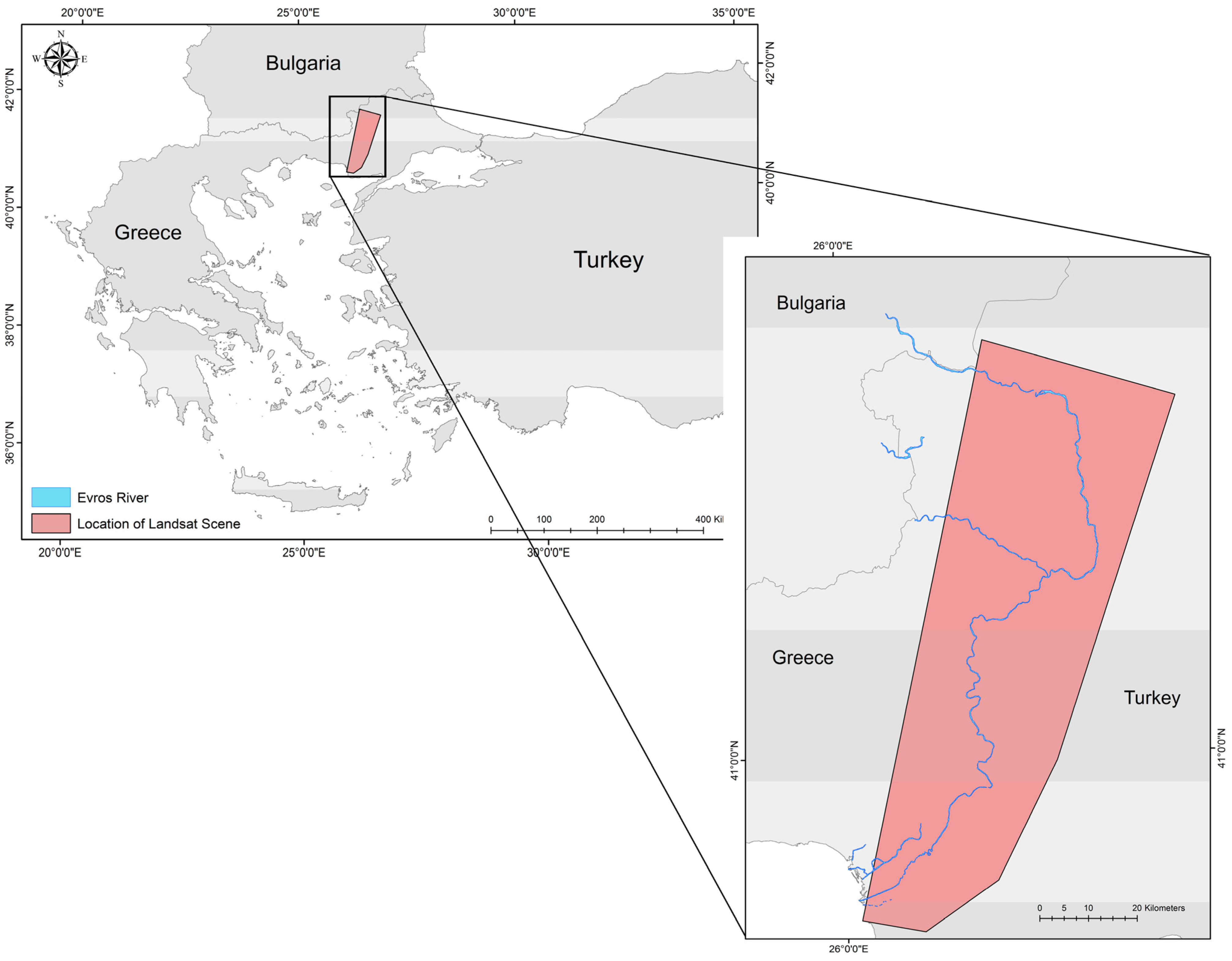
54]. In this context, this study aims to compare the performances of the SVMs and rkFDA methods in extracting flood areas in a fragmented and highly heterogeneous Mediterranean environment. As a case study, the Evros/Maritsa River floodplain located on the border of Greece and Turkey is used.
3. Methodology
In this study, both the SVMs and rkFDA were chosen as classifiers for building different supervised architectures for obtaining classification of the flooded area using Landsat TM images. The motivation of using kernel-based classifiers such as the SVMs and the rkFDA used herein was their intrinsic ability in dealing with non-linear classification problems. They also provide tools to easily control over-fitting during training of the classifier, in contrast to many neural networks architectures which may be hard to train. The remainder of this section describes in detail the models and the steps taken in extracting the flooded areas from the Landsat imagery.
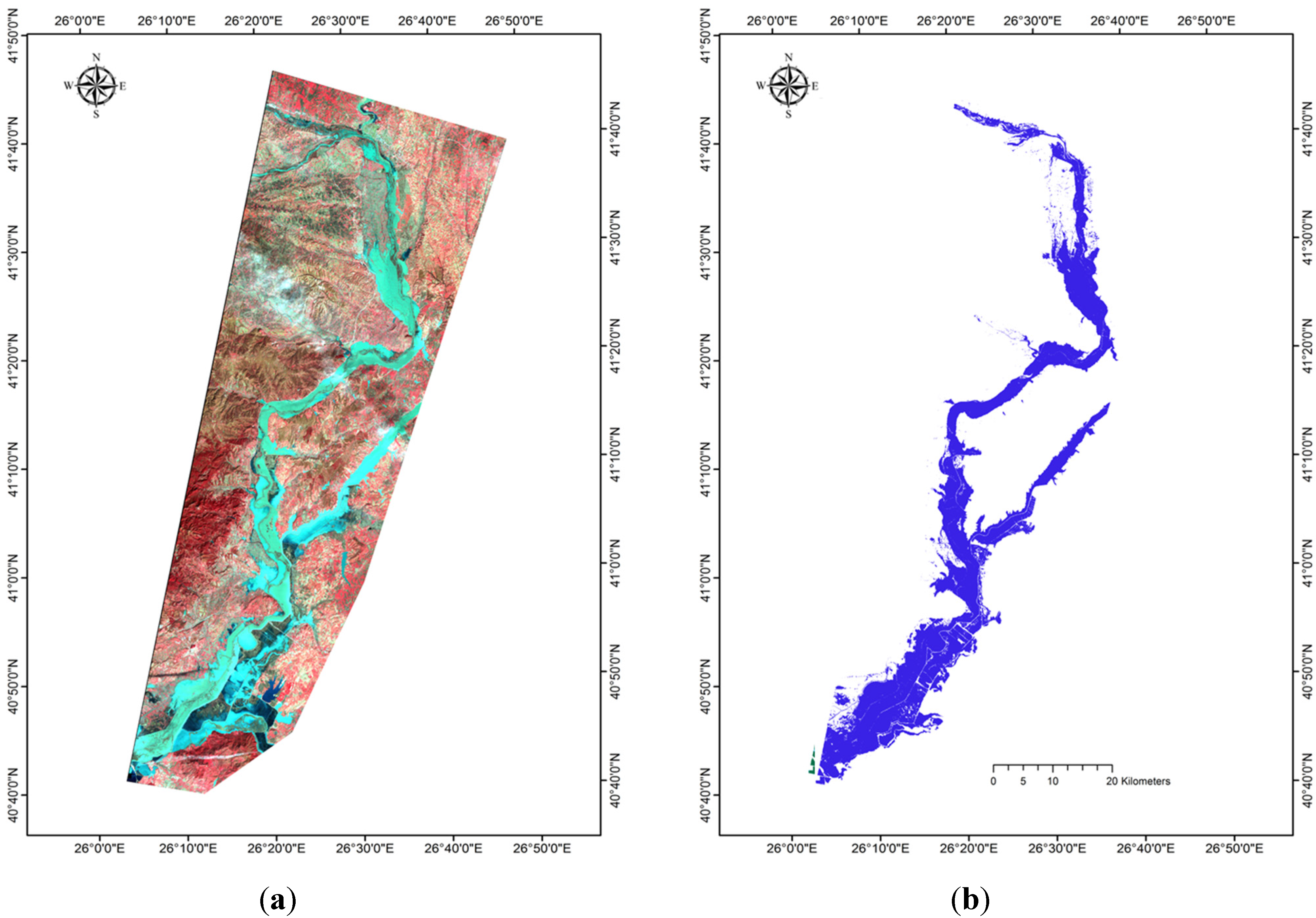
Figure 2.
(a) False colour composite (RGB = 4-3-2) of the post flood Landsat TM imagery acquired on February 19, 2010, flooded area in cyan; (b) Flooded area reference estimate obtained from the Greek Payment Agency (OPEKEPE).
Figure 2.
(a) False colour composite (RGB = 4-3-2) of the post flood Landsat TM imagery acquired on February 19, 2010, flooded area in cyan; (b) Flooded area reference estimate obtained from the Greek Payment Agency (OPEKEPE).
3.1. Support Vector Machines
Support Vector Machines (SVMs) are a non-linear and non-parametric large margin classifier implementing Vapnik’s structural risk minimisation principle [
35,
64]. SVMs separate the samples of different classes by finding the separating hyperplane related to maximal margin minimising the hinge loss function [
65]. Such a solution guarantees a minimal generalisation error. By using non-linear kernel functions (e.g., Gaussian Radial Basis Function (RBF), polynomial) the SVMs implicitly work linearly in a higher dimensional space, corresponding to a non-linear solution in the input space. Such mapping into the higher dimensional kernel space is implicitly performed by a kernel function k(•,•), evaluating the dot product between mapped samples[
64]. For the standard binary SVMs formulation implemented in this paper, the hyperplane f(x) = w'x + b optimally separating the
N training examples x belonging to two classes y ∈ {−1, +1}, is found by minimising:
The slack variables ξ allow some training errors, guaranteeing robustness to noise and outliers.
C corresponds to a user selected hyperparameter controlling the complexity of the model, acting as a trade-off parameter between non-linearity and number of training errors. This quadratic optimisation is solved by introducing Lagrange multipliers α to obtain the following dual form:
When the optimal solution of the latter optimisation is found,
i.e., the
α, labels of unknown test samples x
t are predicted by the side of the margin in which they lie by the following expression:
Note that standard SVMs are sparse in the
α coefficients, so the final solution may be equivalently expressed only by the samples having a corresponding non-zero α. These samples are called support vectors, and are the ones lying on or inside the separating margins f(x) = 1 and f(x) = −1, as depicted by the black examples in
Figure 3.
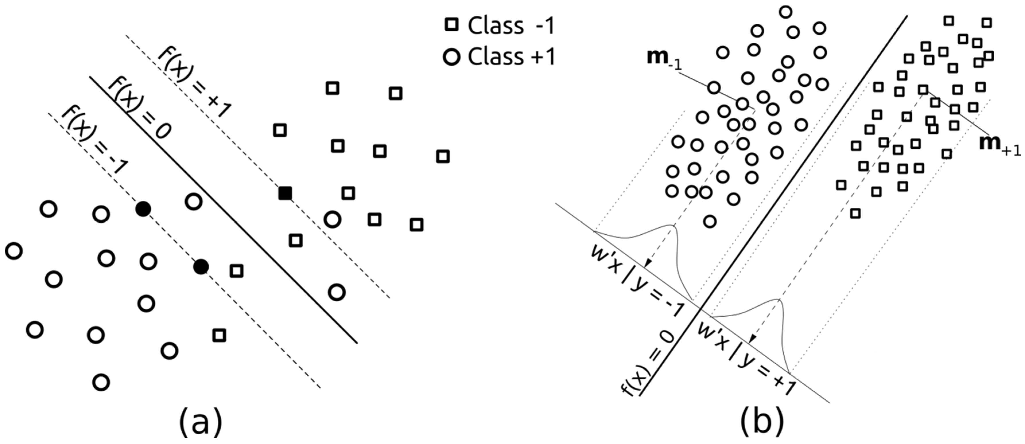
Figure 3.
Graphical representation of the employed methods, (a) Support Vector Machines (SVMs) and; (b) Fisher’s Discriminant Analysis (FDA). For SVMs, black examples denote unbounded support vectors.
Figure 3.
Graphical representation of the employed methods, (a) Support Vector Machines (SVMs) and; (b) Fisher’s Discriminant Analysis (FDA). For SVMs, black examples denote unbounded support vectors.
3.2. Kernel Fisher’s Discriminant
The kernel Fisher’s discriminant classifier is the non-linear version of the Fisher’s discriminant analysis ([
47,
66]). The linear FDA aims at finding a uni-dimensional projection of the training pixels {x
i, y
j} that maximally separates the samples belonging to the two classes y ∈ {−1, +1}, as illustrated in
Figure 3. The decision function is expressed as for the SVMs,
i.e., a linear form f(x) = w'x + b. The optimal direction
w is found by optimising the following Rayleigh ratio:
where
Sb and
Sb are the between and within-class scatter matrices, as:
where
c denotes the class index so that m
c is the average of class
c and
nc indicates the number of examples belonging to it. The optimal
w obtained defines the projection of the samples where the distance between the class averages is maximised, and the average distance of each sample to its centre of mass is minimised. The decision function’s bias term
b is defined implicitly by
b = 0.5 (
m1 −
m−1), respectively. As for SVMs, the sign of the decision function provides the label of the test samples
xt.
For the kernel-based extension, the within and between scatter matrices are reformulated by using kernel functions. By implementing such transformation, the Rayleigh ratio to be optimised in the higher dimensional kernel space is:
where:
m
cφ is the average of the pixels belonging to class
c computed in the kernel feature space as m
cφ = 1/
nc K1
c with 1
c the vector of class indicator (1 if the sample belongs to class
c and 0 otherwise). Note that the kernel matrix has entries K
ij = k(x
i,x
j). As for the non-linear SVMs, kFDA builds on the assumption that by working with samples mapped in some higher dimensional space, a linear separation is achievable, which in turn corresponds to non-linearity in the original input space.
To solve the ratio maximisation problem for the kFDA, one can introduce the Lagrange multipliers
λ and equating to 0 the derivative of the obtained expression with respect to the weight vector
w. Then, one can solve the generalised eigenvector problem Q
α =
λR
α and retaining the eigenvectors
α corresponding to the largest eigenvalues
λ [
58,
67]. Since the problem of estimating covariance structures in a possibly infinite dimensional kernel space using a finite set of samples is ill-posed, R has to be regularised to ensure its non-singularity [
47,
48,
68]. The introduction of a regularisation parameter
ρ is made as R
regu = R + ρ I, where I is the identity matrix of size
N ×
N and
ρ is the penalty parameter to be tuned by the user. The regularised kFDA (rkFDA) solves the generalised eigenvector problem by replacing R with R
regu. When classifying a previously unseen test pixel x
t, its class is given by the sign of the decision function:
The FDA classifier may be seen as a first supervised dimensionality reduction step, maximising the class separability, followed by a minimum Euclidean distance classification. The classifier first finds the subspace in which classes are optimally discriminable, and then a decision function is built by thresholding the line linking the centre of mass of the two classes. The accuracy thus relates to the algorithm ability to find the proper orientation and position of the decision function.
3.3. Flooded Area Classification
Before image classification, each Landsat TM spectral channel of the acquired image was rescaled to zero mean and unit standard deviation. It is important to note that even if the relative importance of the channels is changed, the classifier will converge to an optimal solution. To see this, it suffices to see the form of the decision function, in which the contribution of each sample to the final solution is weighted by the
α term. Thus, by changing the scaling of the input space, the
α will change accordingly, providing the same solution, up to a scaling factor. Furthermore, by using kernels, the scaling of the data is implicitly taken into account by selecting appropriate kernel functions and corresponding hyperparameters. Still, data scaling may influence the speed of convergence of the solver used to train the model [
69].
In this paper, we encoded the flooded area mapping as a binary classification problem. Specifically, we recoded the target class “flood” as being labelled as {y = +1|flood} and the “not flooded” class as {y = −1|not flooded}. By taking N labelled pixels vectors we could then form a learning set X composed by N pairs {(x1, y1 ), ... , (xn, yn )}, yi ∈ {−1, +1}, where yi is the label corresponding to pixel xi. We employed a Gaussian RBF kernel of the form k(xi,xj) = exp(−||xi − xj||2 )/2σ2, for both SVMs and rkFDA. To optimise the free parameters of the classifiers, we employed a five-fold cross validation scheme, to tune the kernel bandwidth and penalisation C of the SVMs, and the bandwidth and ρ of the rkFDA, respectively. For both classifiers, we employed different training sets sizes, in order to test the sensitivity of the system to the learning set size. This number was varied in {10, 50, 100, 200, 250, 500, 1000} pixels for each class. Note also that the test set, on which the generalisation ability was evaluated, was kept fixed by randomly selecting the 70% of all the available labelled samples prior to the experiments. We then extracted the training samples from the remaining 30%. The experiments were repeated 10 times with independent realisations of the training set.
To provide a comparison with a baseline flooded area extraction method, the approach relying on the Normalised Difference Water Index (NDWI) from [
70,
71] was implemented. In our setting, we estimated the threshold on the NDWI using the well-known Otsu’s histogram thresholding method [
72]. We also tested a fully supervised thresholding strategy, providing very similar results. SVMs’ classification was implemented using the MATLAB interface of the LibSVM library [
73]. For the rkFDA, we solved the generalised eigenvector problem using the MATLAB built-in ARPACK library, exploiting an iterative deflation scheme. The remaining parts of the classifications steps were implemented in MATLAB R2010b. Post-processing of the maps and visualisation was carried out by using the ArcGIS 10.2 software platform. The execution time for both rkFDA and SVMs was comparable. For the experiments relying on 200 training samples illustrated in
Table 1, the execution time (including model selection, prediction on the whole image and accuracy assessment) was in the order of 5 min on a standard laptop setup (a quad core system, i7, with 16 GB RAM).
Table 1.
Average error matrices of the three classification methods using models trained on 200 pixels per class. Accuracy values are expressed in (%). F—Flooding, NF—Not flooding, UA—User’s Accuracy, PA—Producer’s Accuracy, OA—Overall Accuracy, K—Kappa coefficient.
Table 1.
Average error matrices of the three classification methods using models trained on 200 pixels per class. Accuracy values are expressed in (%). F—Flooding, NF—Not flooding, UA—User’s Accuracy, PA—Producer’s Accuracy, OA—Overall Accuracy, K—Kappa coefficient.
| rkFDA | SVMs | NDWI |
|---|
| Linear | Linear | |
|---|
| | F | NF | UA | | F | NF | UA | | F | NF | UA |
| F | 3,500,651 | 27,250 | 99.23 | F | 3,484,453 | 20,244 | 99.42 | F | 3,493,275 | 85,151 | 97.62 |
| NF | 144,008 | 729,572 | 83.52 | NF | 160,206 | 736,578 | 82.14 | NF | 151,384 | 671,671 | 81.61 |
| PA | 96.05 | 96.4 | | PA | 95.6 | 97.32 | | PA | 95.85 | 88.75 | |
| OA | 96.11 | AA | 96.23 | OA | 95.9 | AA | 96.46 | OA | 94.63 | AA | 92.30 |
| K | 0.871 | | | K | 0.866 | | | K | 0.818 | | |
| RBF | RBF | | | | |
| | F | NF | UA | | F | NF | UA | | | | |
| F | 3,485,275 | 6690 | 99.81 | F | 3,476,370 | 5205 | 99.85 | | | | |
| NF | 159,384 | 750,132 | 82.45 | NF | 168,289 | 751,617 | 81.71 | | | | |
| PA | 95.63 | 99.12 | | PA | 95.38 | 99.31 | | | | | |
| OA | 96.23 | AA | 97.35 | OA | 96.06 | AA | 97.35 | | | | |
| K | 0.877 | | | K | 0.873 | | | | | | |
3.4. Accuracy Assessment
The computation of error matrix statistics, namely the overall accuracy (OA), user’s (UA) and producer’s (PA) accuracy, and the Cohen’s Kappa (K) statistics, were used to assess the different classification methods’ performance (Equations (9)–(12); [
74]). OA expresses the probability that a pixel is correctly classified by the thematic map and is given as percentage (%), which is also interpreted as a measure of the overall classification accuracy. K measures the actual agreement between reference data and the outcome of the classifier used to perform the classification, versus the chance of agreement between the reference data and a random classifier. The percentage of correctly classified ground classes by the analyst is expressed by the PA, which defines the measure of pixels omitted from its reference class (omission error). Likewise, UA expresses the percentage of pixels of a category that do not “truly” belong to the reference class, but are committed to other ground truth classes (commission error) [
75]. In computing the above statistical measures, approximately 4.4 million validation pixels (
i.e., 70% of the whole reference map shown in
Figure 2b) were employed. To ensure consistency in our comparisons, the same set of validation points was used in evaluating the accuracy of all thematic maps produced from the implementation of the different classifiers.
In addition, the flooded area map derived from each classification method was compared against the reference flooded area estimate. Flooded area detection accuracy was thus evaluated following the rationale of Kontoes
et al. [
76], where, following this approach, accuracy of the flooded area estimates were expressed in terms of detected area efficiency (DAE), skipped flooded area rate (SFA, omission error) and false flooded area rate (FFA, commission error). These accuracy metrics were calculated on the basis of the following formulae:
In the above equations, DFA is the Detected Flooded Area (common area between the generated flooded area polygon and the reference polygon), FFA is the False Flooded Area (the area included in the generated flooded area polygon but not in the reference polygon) and SFA is Skipped Flooded Area (the area included in the reference polygon but not in the generated polygon).
Note that our validation map includes mixed pixels and flooded pixels covered with emerged vegetation. In our implementation, as we do not have a flag indicating those pixels, mixed flooded pixels were included in both training and testing sets. However, by selecting those samples at random and by repeating experiments using multiple training sets realisation, their effect on the classification procedure is averaged out when estimating the accuracy metrics.
4. Results
The statistical measures used in evaluating the accuracy of the derived flooded area maps produced by the different techniques implemented are summarised in
Table 1. The corresponding thematic maps derived from the implementation of these classifiers to the TM post-flood imagery are also illustrated in
Figure 4 and
Figure 5. Note that these maps were obtained by employing 200 pixels per class, thus a total of 400 examples for the binary flood mapping task. This number has been chosen in order to assess the behaviour of the system in a best-case scenario, which makes the comparisons of the derived flood maps fair. Note that the number of training samples can be increased by photointerpretation with little effort. The accuracy obtained with unsupervised flood area detection based on the NDWI automatic thresholding is illustrated in
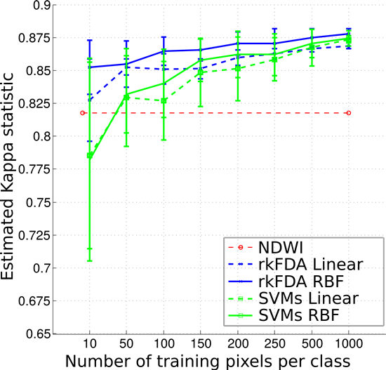
Figure 6. This plot shows that this strategy performs comparably to the rkFDA and SVMs models trained on 10–100 pixels, although being significantly less accurate when training supervised models with more samples. Furthermore, by employing larger training sets only minor improvements in accuracy are observed.
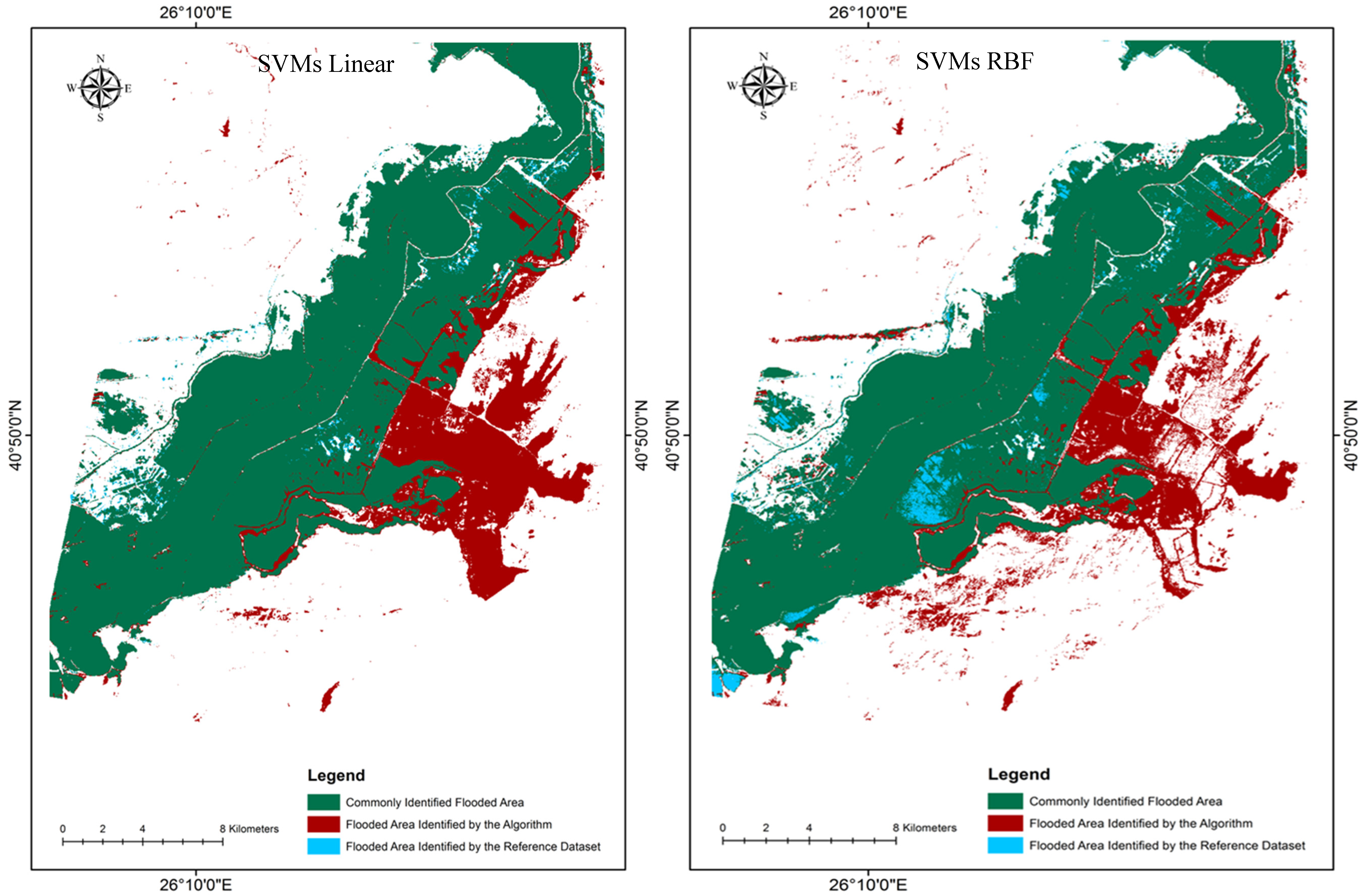
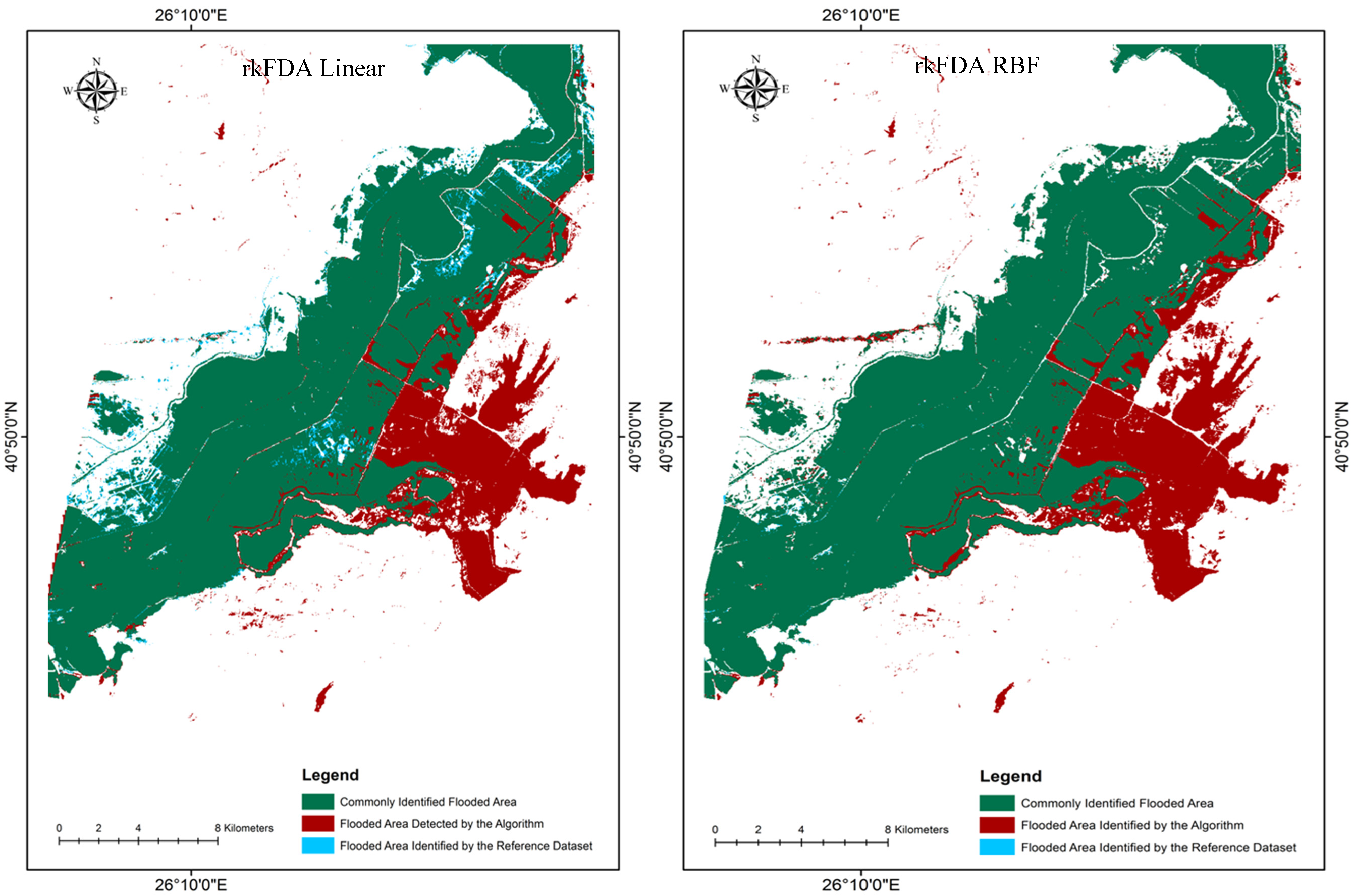
A visual comparison of the derived flooded area maps from the different methods investigated (
Figure 4 and
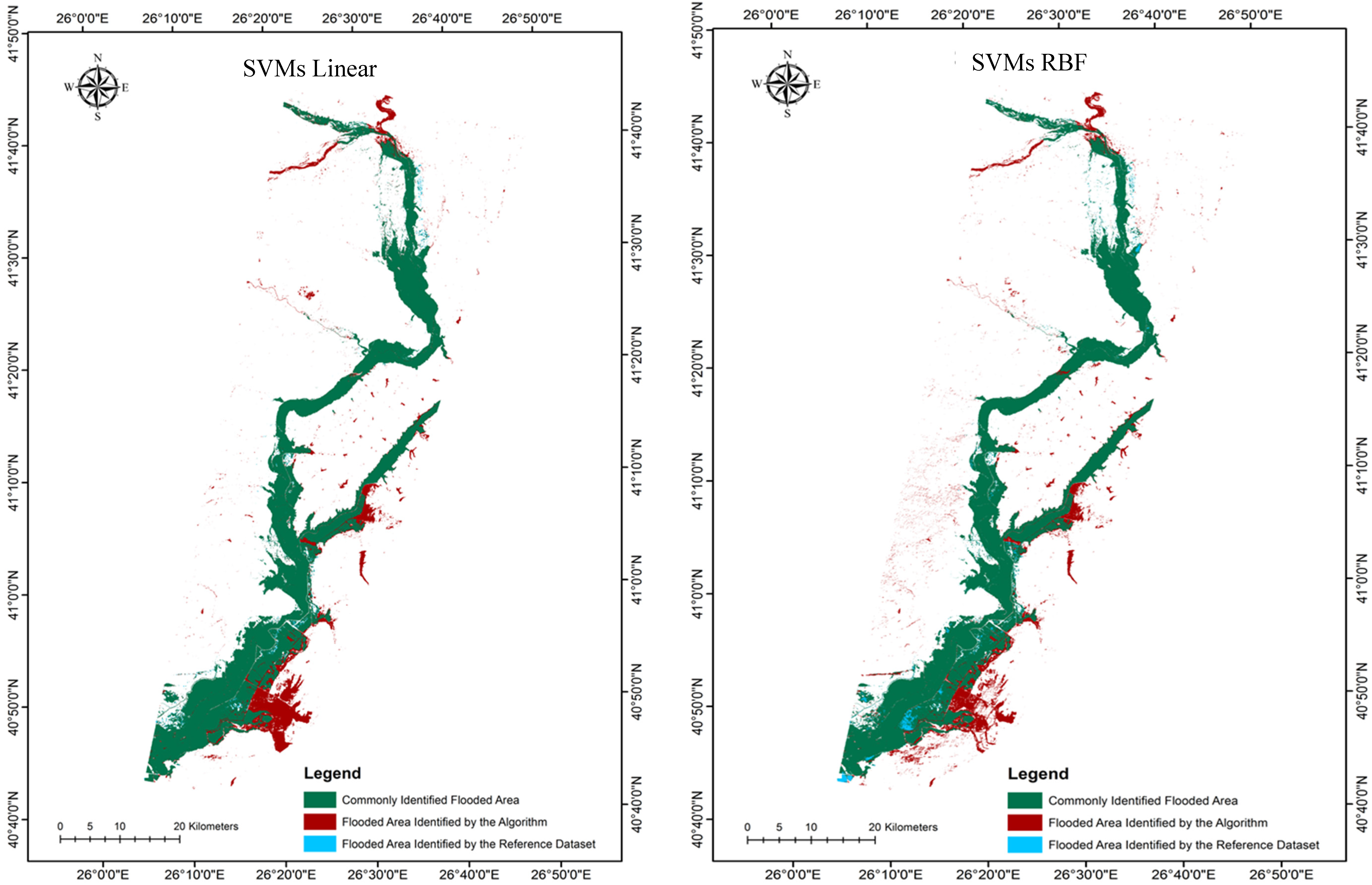
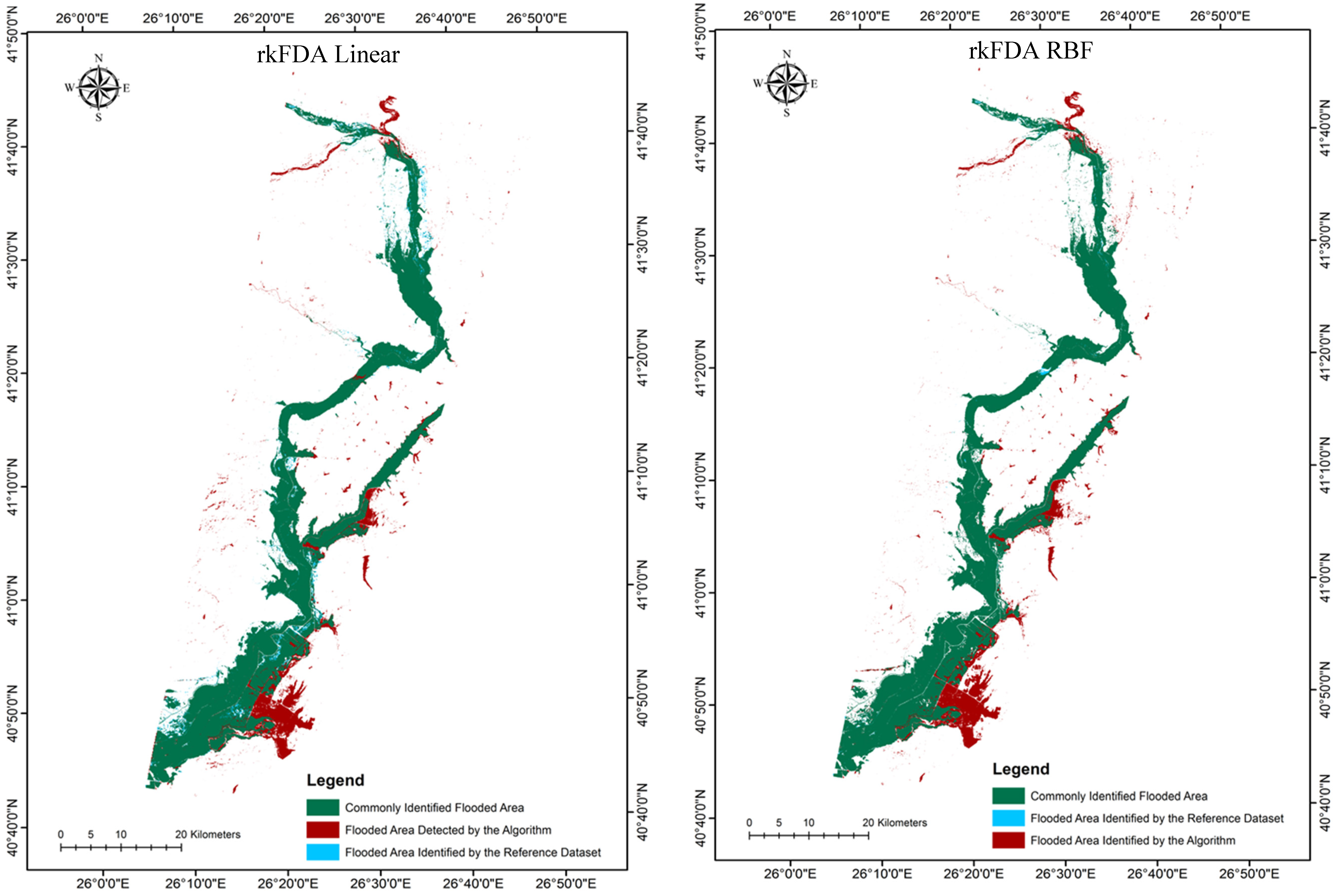
Figure 5) shows that there are a number of outlying pixels identified as flooded areas visible in all estimations that are not actually present on the validation map. The majority of these outlying pixels are located to the south east of the flooded area and are most prominent in the SVMs non-linear estimation.
Figure 4.
Flooded area maps derived from the implementation of the different classification algorithms and parameterisation scenarios implemented.
Figure 4.
Flooded area maps derived from the implementation of the different classification algorithms and parameterisation scenarios implemented.
Figure 5.
Subset of the southern region of the flooded area maps from each classification scheme.
Figure 5.
Subset of the southern region of the flooded area maps from each classification scheme.
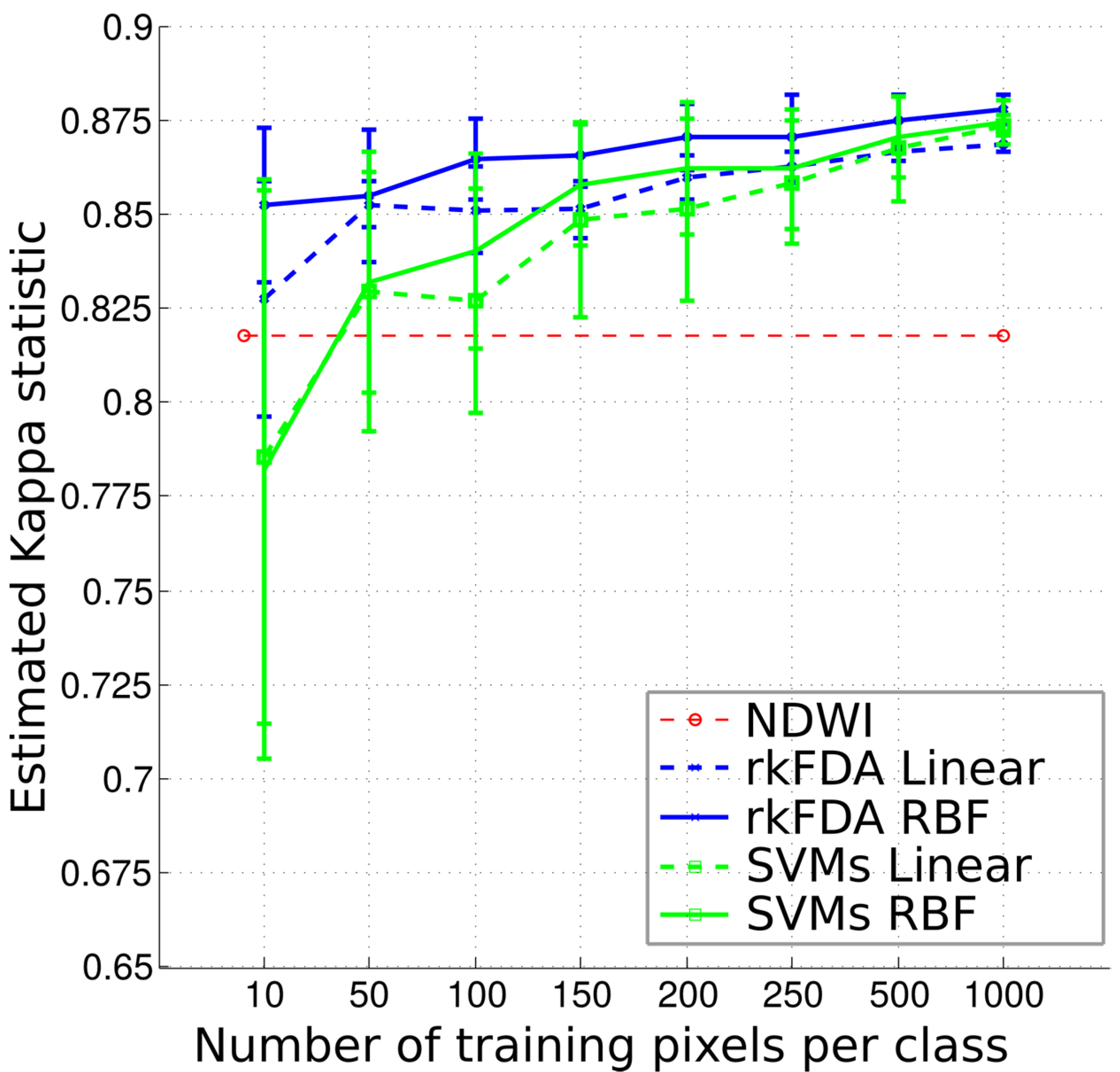
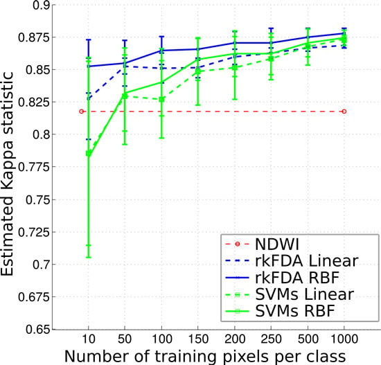
Figure 6.
Classification accuracy as measured by the K coefficient as a function of the training samples employed.
Figure 6.
Classification accuracy as measured by the K coefficient as a function of the training samples employed.
In terms of absolute accuracy assessment, OA and K results were 95.9% and 0.866 for the linear SVMs, 96.11% and 0.871 for the linear rkFDA, 96.1% and 0.873 for the non-linear SVMs, and 96.23% and 0.877 for the non-linear rkFDA. These values signify high accuracy for all flooded area maps and a low variance between the accuracies of the different classification methods. On the basis of the OA and K results alone (
Table 1), the rkFDA performed slightly better than the SVMs for both the linear and non-linear algorithms. Furthermore, non-linear algorithms were more accurate for both classification methods. NDWI thresholding provided less accurate results, in particular for the detection accuracy of the “not flooded” class. Results suggest that the most accurate mapping method when using 200 training examples per class resides in the non-linear kFDA classification (OA 96.23% and K 0.877). However, the difference between classification methods was minor.
As can also be seen from the UA comparisons, for both classification methods false alarm rates are reduced by the SVMs, showing an increase of 0.04% in accuracy using non-linear and 0.19% using linear algorithms depicted by the “flood” class user accuracies. Furthermore, the SVMs classifier performed better in detecting the “not flood” class, yet with a minor difference in terms of variance in comparison to the other technique. Even if the rkFDA classification performs less accurately in detecting false alarms, it provides a higher detection ratio for the flooding class, corresponding to fewer missed detections of the flooded area, with an increase of 0.25% using non-linear and 0.45% using linear algorithms in PA. However, missed detection performance for the SVMs is very close. The SVMs and the rkFDA performed similarly on all the computed scores, except for the PA of the nonlinear classifiers which increased by 1.99% and 2.72%, respectively. As mentioned, the NDWI PA score was largely outperformed by the two classifiers (10.37% and 10.56%, respectively) indicating that it is significantly less reliable in detecting unflooded areas. Globally, the average per-class accuracy (AA) is ~1% higher for the nonlinear models over the linear ones and ~5% over the NDWI thresholding. Linear models appear to be more conservative in the prediction of flooded pixels (detection rate higher than the non-linear scheme) in both classification techniques as reflected in the higher user accuracies. It also clearly appears that NDWI based methods provide lower scores for the considered training set sizes.
The overall accuracy values may seem very close, but are biased by the very large number and unbalanced number of samples per class. These differences in accuracy become more striking when looking at
Figure 6, illustrating the evolution of the K coefficient as the size of the training set grows. As a first observation, as the number of samples employed to train the classifiers increases, the accuracy grows. However, when employing 150 or more samples per class, the Kappa coefficient shows a stable accuracy, and only the standard deviation of the outcomes decreases. Furthermore, for small sample sizes, the SVMs show a generally lower accuracy and higher standard deviations. On the contrary, the rkFDA, and in particular the non-linear variant, shows a very stable behaviour, also providing high accuracy for the tested situation, compared to the situation exploiting more than double the training samples. In this setting, being unsupervised, the NDWI shows a constant accuracy.
Apart from the evaluation on the basis of the error matrix statistics (UA, PA—
Table 1), the classified flooded areas were assessed against the reference flooded area estimate. Absolute differences in flooded area estimates between the reference and the SVMs classifications methods varied from 1.2%–2.7% and between the reference and the rkFDA classifications from 1%–3.6%, respectively, indicating a close agreement between the reference polygon and each classification output. Notably, highest agreement in the total flooded area estimates was observed in the case of the rkFDA RBF implementation, followed by the SVMs Linear, SVMs RBF and rkFDA linear classifications, respectively.
As illustrated in
Table 2, highest DFA was also observed for the case of the rkFDA RBF classifier implementation, with a common flooded area of 674.74 km
2. Evidently, in terms of skipped flooded area (SFA), results were proportional to the common flooded area estimates; similarly, the best result
i.e., the lowest rate of skipped area (0.032%) was obtained in the case of the rkFDA RBF scenario (6.49 km
2), also evidenced in the omission error percentage (0.010%). Comparably low SFA and omission errors were also evident for the SVMs linear classification (SFA = 8.37 km
2, Omission Error = 0.012%), whereas the highest rate was attributed to the rkFDA linear scenario with 24.78 km
2 (omission error = 0.036%) of skipped flooded area. Evaluation of the subset of the study area illustrated in
Figure 5 also clearly depicts an increase in flooded area identified by the reference polygon but not the algorithm for both the SVMs linear and rkFDA RBF classifications in comparison to the other two. Yet, in terms of falsely detected flooded area (FFA, commission error), no clear trends in observations were evident, apart from the fact that the rkFDA linear classification algorithm reported the lowest FFA of all scenarios. This is again clearly evidenced in the south eastern region of the study area subset in
Figure 5.
Table 2.
Summary of the flooded area comparisons between our reference dataset and those derived from the implementation of the different classifiers to the Landsat-TM images.
Table 2.
Summary of the flooded area comparisons between our reference dataset and those derived from the implementation of the different classifiers to the Landsat-TM images.
| Classification Algorithm | Detected Flooded Areas (km2) | False Flooded Areas (km2) | Skipped Flooded Areas (km2) | Detection Efficiency Rate (%) [DFA/(DFA + SFA)] | Commission Error (False Alarm Rate) (%) [FFA/(DFA + FFA)] | Omission Error (%) [SFA/(DFA + SFA)] |
|---|
| SVMs Linear | 672.86 | 150.36 | 8.37 | 0.988 | 0.221 | 0.012 |
| SVMs RBF | 662.65 | 144.64 | 18.58 | 0.973 | 0.212 | 0.027 |
| rkFDA Linear | 656.45 | 129.87 | 24.78 | 0.964 | 0.191 | 0.036 |
| rkFDA RBF | 674.74 | 143.92 | 6.49 | 0.990 | 0.211 | 0.010 |
5. Discussion
The implementation of the SVMs and rkFDA classifiers combined with Landsat TM imagery resulted in satisfactory mapping of the flooded area extent in most cases, despite the complex and highly fragmented landscape of our Mediterranean study site. These results confirm those of studies utilising similar techniques [
32,
77]. In both cases, NDWI-based flood mapping was outperformed. However, note that the latter has been implemented in a fully automated manner (
i.e., no training samples were used) and, consequently, its results were competitive, in particular when very few training examples are available for learning. On the basis of results obtained herein from the classification accuracy assessment metrics, variance in performance between the classification methods examined was minimal. SVMs outperformed the rkFDA in false alarm detection rates, meaning that in that respect rkFDA was more accurate in identifying the flooded areas present in the image. However, the difference in OA was indeed minimal using both linear and non-linear algorithms (<1%). Conversely, the rkFDA classification showed higher accuracy in detection of “flooded” pixels, corresponding to fewer missed detections of the flooded area and displayed results comparable to object based approaches [
15,
26,
78]. The reason behind the higher detection rate given by the rkFDA is its ability to explicitly transform the data so that the two classes are maximally separated. This possibly results in a better class separation if the training samples used are representative of the underlying data structure. For SVMs, as they optimise a global binary trade off, the training accuracy is more balanced between the two classes. Overall, the rkFDA classification for flood mapping showed accuracies and performances close to the ones provided by the SVMs, and in the majority of cases improved slightly on these results. More interestingly, the rkFDA consistently provided better results than SVMs for small sample situations. The more variable behaviour of the SVMs may be attributed to how the model exploits the samples during training. In fact, a separating hyperplane is constructed from a small set of pixels, which strongly depends on the representativeness of such a set in relation to the underlying data distribution. In other words, if such a set contains a large proportion of outliers or noise, the separating hyperplane cannot approximate well the true data distribution and consequently provides a separating margin which performs unevenly in terms of generalisation. As the number of samples employed increases, the underlying data distribution is better approximated empirically and SVMs show performances close to an optimal classifier.
The rkFDA shows a much more accurate and stable behaviour in small sample situations. In its linear version, the FDA takes advantage of a prior assumption made on the data, that is, the Gaussianity of the class-conditional distributions (see Equations (4) and (5)). In the case of flood mapping, the “flooding” class forms a small normally distributed cluster, due to the additive imaging noise. The “not flooding” class is much more heterogeneous, as it corresponds to a composition of many different spectral classes and it may be seen as distributed following a Gaussian mixture. By working with kernels, we implicitly extend the same assumption into a higher dimensional space, in which linear rather than nonlinear relationships have to be modelled. As illustrated in Huang
et al. [
45], if the samples of this class cover the underlying data variability, their projection into the kernel space follows a unimodal normal distribution. In this case, the non-linear rkFDA takes advantage of this assumption by further imposing a Gaussian model over the class (Equations (6) and (7). This may be seen as imposing a prior over the class-conditional distribution (the within-class covariance), acting as an additional regularisation term. Coupled to the empirical regularisation of the within class scatter matrix, the rkFDA shows an interesting robustness with respect to small sample situations.
A posteriori, we may also state that the variability of the “not flooded” class, assuming that the “flood” class can be easily modelled, starts to be best depicted from employing 50 training samples per class, as illustrated by the reduced standard deviation of the accuracy plot of
Figure 6. However, note that depending on the data at hand and since different classification problems may require different modelling tools or different assumptions, these observations may not be generalisable to arbitrary tasks. Observing flood extent delineation from a uni-temporal perspective reduces the task to a binary classification of flood extent against the rest, where standard single image classification methods can easily detect pure pixels [
32]. However, issues related to mixed pixels and water colour can limit the effectiveness of a uni-temporal model in more fragmented environments. Although nonlinear methods have shown superior ability in correctly classifying mixed pixels and emerged vegetation, as illustrated by the larger accuracy measures; this particular aspect deserves a specific study, provided an appropriate ground truth map is available. One possible solution to this issue is to carefully include a covering of the observed variability of the data (paying attention to all the spectral channels) in the training set samples. This way, the statistical distribution between training and test samples is maximally matched and the learning algorithm may unbiasedly learn the correct decision function.
Additional improvements may be given by considering a multi-temporal approach, which can exploit the multi-temporal dependences to solve the mixed and ambiguous pixels exhibited by a single image setting. In most situations, it is not possible to differentiate permanent standing waters from flood waters using only a uni-temporal image as source of information. The only situation in which permanent standing waters are discriminable from the flood waters, from a uni-temporal perspective, is when there is a spectral difference (
i.e., different water colours induced by different turbidity levels). In these situations, a classifier may be trained to differentiate waters if enough training samples are available for both water classes. If the two kinds of waters are very similar in spectrum, or turbid waters cover also permanent standing waters, there is no possibility to differentiate them on the basis of a single acquisition. Including a multi-temporal approach, in addition to specifically annotated data, would help address such issues and would avoid the misleading inclusion of the permanent standing water bodies as flooded regions, which may require additional non-linearity within the models [
32]. A further limitation of a uni-temporal approach is the fact that floods are wave phenomenon and all satellites have their repeating intervals. Generally, the time of acquisition of satellite data does not coincide with the time of flood peak which is related to the maximum inundation area [
79]. This lack of timeliness may undervalue the possible usage of uni-temporal satellite data for flood mapping. However, a number of studies have shown such methods to be successful [
32,
53,
80]. Notably, a study by [
80] indicated that it is possible to successfully use remotely sensed data acquired days after a river’s crest to capture most of the maximum extent of a flood. In their study, an image acquired nine days after the flood event captured over 90% of the flood extent identified in a classification from two days following the event. Such results indicate the use of remotely sensed data acquired days after a river’s crest to capture most of the maximum extent of a flood should somewhat reduce the requirement to have concurrent remotely sensed data.
Non-linear models drastically reduced the false alarm rate and improve the “not flood” detection, while also coping with the high spectral variance of within-class heterogeneity explaining the higher accuracies exhibited by the non-linear models. The rkFDA classification method appears to be an effective and robust method for flooded area mapping. However, on the basis of our study results, it seems that it cannot be guaranteed that rkFDA is generally more accurate than SVMs when implemented in other scenarios or in landscapes that contain different spectral classes and mapping characteristics to the study site. This is something requiring further investigation. In our experiments, a McNemar test showed that maps obtained with nonlinear models are statistically better than linear counterpart (p < 0.001), conditioned on the method (e.g., linear SVMs versus non-linear SVMs or linear rkFDA versus nonlinear). Note that linear and non-linear SVMs trained on 10 and 50 training examples were not statistically dissimilar. Similarly, McNemar test illustrated that rkFDA maps are statistically better than the SVMs, conditioned on the fact that the algorithm is linear or nonlinear. However, note that a mean test over the K values for the 10 different outcomes showed that all the methods, given a specific training set size, were not statistically superior. NDWI results statistically inferior for training sets larger than 150 samples. Possible reasons for the inferior performance from the NDWI thresholding for the detection of the “not flooding” class are to be searched in the high degree of mixing between the “flood” and “not flood” distributions. Furthermore, this mixing can be increased by the nature of the “not flood” class. Since this land cover is composed by different spectral classes with possible heterogeneous responses in the NDWI domain, the mixing between distributions may further increase, resulting in a bad separability between boundary regions (e.g., wet non-flooded areas and low depth flooded areas).
In terms of computational complexity, the methods examined herein were comparable, resulting in similar running times. For both SVMs and rkFDA, time complexity is mainly controlled by the number of training samples. By reducing this number, classification maps may be obtained faster, but obviously losing accuracy. In such applications, the user is often required to manually annotate regions of the image corresponding to the spectral classes to be discriminated. A possible strategy to obtain compact and informative training sets is to select areas which show different visual aspects of the same class, such as different water colours, or carefully including all the possible ground covers of the “not flooding” class [
81]. In general, results obtained for the SVMs, rkFDA and NDWI are in line to what is observed in the EO domain [
47,
82]. This confirms the suitability of the adopted tools for flood mapping, as discussed.
6. Conclusions
In this paper, the behaviour of two contemporary and very promising machine learning techniques was explored for mapping flooded areas when implemented with freely distributed EO datasets. Investigation was implemented in a complex and challenging Mediterranean landscape using Landsat TM imagery acquired shortly after the flooding event. In particular, we assessed the effectiveness of SVMs in flooded area extraction and also provided an alternative to them, the regularised kFDA. To our knowledge, very few similar studies have been performed in the past, if any, particularly so in a highly fragmented landscape such as that of the Evros River basin.
Results from our study showed very interesting properties in terms of the ability of the classifiers to capture the flooded areas. Differences in the assumptions about class separation are reflected in the different reported repartition of users’ and producers’ accuracies, suggesting rkFDA to be slightly more accurate than the SVMs and clearly outperforming NDWI-based flood detection. When looking at the overall accuracy differences seemed minor. However, it should be noted that other accuracy measures were significantly lower for the NDWI based approach: for instance, NDWI producer accuracy for the “not flooded” class was around 10.5% less accurate than the rkFDA and SVMs. Furthermore, the average per-class accuracy was 92.30% for the NDWI, 96.23% for the linear rfFDA, 96.46% for the linear SVMs, while 97.35% and 97.35% for the nonlinear classifiers, respectively. Therefore, supervised classifiers exhibited a significant improvement over the NDWI thresholding. Finally, notably, the K index was also 0.05–0.06 lower for the NDWI, which may be regarded as significant. Generally, the overall accuracy is not the optimal metric to assess the applicability of a classifier, as it is biased by large unbalanced classes. Overall, the NDWI was outperformed by both classifiers. However, due to pixel-wise classification, spurious errors and small patches of false alarms, mainly caused by under-representation of such areas into the training set corresponding to the unflooded areas, can provide limitations to the accuracy of these techniques. To solve these problems, future research is required towards the direction of dealing with intelligent and automatic sampling strategies to better represent the class statistics into the training set. Possible approaches may be found in coupling clustering or mixture models to learn the statistical distribution of the data with supervised classifiers. In future work, it will also be worth exploring specific feature extraction strategies for flooded area mapping. Specifically, focus should be placed on extracting information correlated with the flooded areas (e.g., NDWI) and providing multi-scale smoothing to include the spatial correlation of the flood area into consideration. Furthermore, taking into consideration the complexity of the study site characteristics, performance of the techniques examined here demonstrates the feasibility of their use in flooded area mapping of other fragmented heterogeneous landscapes globally.
The use of machine learning models for classification of pixels into flooded and not flooded classes resulted in accurate maps by both examined techniques, which provide a reliable source of information for decision makers and local policy agencies. Our study contributes to a better understanding of the suitability of the examined machine learning approaches in natural hazards mapping and floods in particular. This is extremely important, given that floods are one of the most significant natural disasters in our planet affecting and often threatening different aspects of human life. Furthermore, our study advocates as well the appropriateness of the examined machine learning approaches for use with freely distributed Landsat imagery for mapping flooded areas in a cost-effective, semi-automatic and rapid manner. This is of considerable scientific and practical value to the wider scientific community, given the continued open access of observations from this satellite globally.


