Statistical Modeling of Soil Moisture, Integrating Satellite Remote-Sensing (SAR) and Ground-Based Data

Abstract

We present a flexible, integrated statistical-based modeling approach to improve the robustness of soil moisture data predictions. We apply this approach in exploring the consequence of different choices of leading predictors and covariates. Competing models, predictors, covariates and changing spatial correlation are often ignored in empirical analyses and validation studies. An optimal choice of model and predictors may, however, provide a more consistent and reliable explanation of the high environmental variability and stochasticity of soil moisture observational data. We integrate active polarimetric satellite remote-sensing data (RADARSAT-2, C-band) with ground-based in-situ data across an agricultural monitoring site in Canada. We apply a grouped step-wise algorithm to iteratively select best-performing predictors of soil moisture. Integrated modeling approaches may better account for observed uncertainty and be tuned to different applications that vary in scale and scope, while also providing greater insights into spatial scaling (upscaling and downscaling) of soil moisture variability from the field- to regional scale. We discuss several methodological extensions and data requirements to enable further statistical modeling and validation for improved agricultural decision-support.

1. Introduction

1.1. Challenges in Modeling Soil Moisture Using Satellite, Remote-Sensing Data

There are substantial challenges in modeling soil moisture and integrating remote-sensing and ground-based data reliably, given significant spatial and temporal measurement variability and model prediction uncertainty. While soil moisture estimation from Synthetic Aperture Radar (SAR) polarimetry (or scatterometer) data is a topic that has been investigated for over 30 years, with numerous papers having been written and statistical approaches developed, SAR and models using such data are nonetheless continuing to be re-configured, improved and extended given the wider availability of SAR data and to address a rapidly growing demand in its use in a broad set of industrial and environmental applications [1]. More reliable predictions of soil moisture are needed when optimizing crop water use and validating satellite remote-sensing/earth observational information [2,3]. Agricultural crop irrigation scheduling, disaster response and water management during droughts or flooding extreme events, soil erosion and pollution monitoring making use of hydrological models, all require reliable predictions of daily and field-scale soil moisture.

Soil moisture is a key variable used to calibrate complex agroecosystem models and for forecasting crop yield at the regional scale, and increasingly hydrological and agroecosystem models are being used in environmental decision support and policy-making. Yet, despite its broad importance, field-scale soil moisture data are often not available or closest neighbor values are used when modeling hydrological and biochemical processes or when calibrating regional-scale predictions generated by complex agroecosystem models. This is, in part, due to constraints and limitations in acquiring and assembling such data over large regions and across sufficient time-periods; the acquisition process is not only costly, but labour intensive, and has high variability when upscaled from the field, to landscape, up to the regional-scale [4–6]. Instead of relying on direct soil moisture information validated against remote-sensing data, auxiliary predictions are often substituted based on indirect, interpolative or extrapolative assumptions that may not be statistical accurate, nor readily verifiable. Coupled with such challenges, there is also a lack of sufficient understanding that is required to optimally: (1) predict soil moisture across sites or regions where data are sparse or not available, and (2) generate predictions that are robust under different environmental and land-management conditions, given high observed variability at the field-scale, as well as, high stochasticity linked with changing weather patterns and the timing and severity of rainfall events.

Soil moisture is a process that is strongly time and space dependent. Nonetheless, there are advantageous properties of soil moisture variability that enable one to use available data, obtained at specific locations, to predict for unobserved times and spatial locations, namely: (1) a deterministic relationship between the high “dielectric constant” of water and variation in horizontal and vertical “backscatter” in remote sensing (hereafter denoted by RS) data; (2) reproducible spatial-temporal patterning and trends that arise, for example, from spatial variation in soil type and characteristics and/or seasonal patterns of stochastic rainfall events, and (3) significant dependence between soil, vegetation, climate/atmospheric, topographic and other environmental variables in time and space.

1.2. Research Objectives

In this paper, we present a flexible, integrated statistical-based modeling approach to improve the robustness of soil moisture data predictions. We apply this approach in exploring the consequence of different spatial correlation assumptions and choice of leading predictors and model structures. Previous investigations that have applied statistical models have not included variable (covariate) selection, spatial correlation aspects, and propagation uncertainty [7–12]. We demonstrate our approach using a multi-site data across an agricultural study area in Canada. This selected data was associated with conditions of high environmental variability and homogeneous terrain and thus provided a strong “stress-test” for predictive-based modeling. Our aim was to generate new findings and insights on the: (1) selection of different predictor variables from a set of competing ones linked with available RS data, expert knowledge and semi-empirical algorithms, and (2) selection of different models with differing spatial correlation assumptions. A statistical modeling approach that integrates variable and model-based selection offers greater flexibility to enable models to be more broadly applied across a wide range of applications. The approach we describe also deals with overfitting in the multivariate context. We utilize a broad set of statistical validation measures (e.g., AIC, BIC and DIC criterion), including cross-validated RMSE (CVE) and correlation (CVR) for evaluating the performance of model soil moisture predictions.

The paper is structured as follows: Section 2 includes a summary of the data collection methods. Section 3 defines our statistical modeling approach and the procedures we applied for selecting, optimizing and evaluating the performance of different sets of predictors, covariates, model structures, and spatial dependence. Section 4 presents results on predictor selection and validity, the relative performance of different statistical model structures and the relative influence of spatial correlation on model performance. In Sections 5 and 6 we summarize our findings, their implications and the importance of applying statistical-based modeling that enables automated selection of predictors, covariates, model structural and spatial correlation for optimizing soil moisture predictions and obtaining robust, cross-validated model performance statistics, integrating SAR and gound-based data. We also outline our future work and goals.

2. Study Region and Data Sources

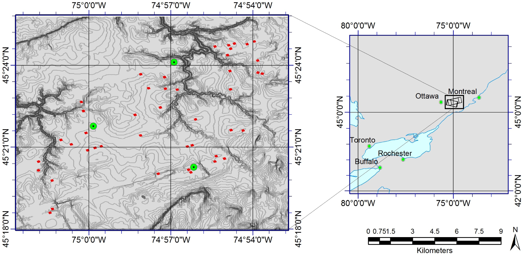
The study was conducted in an agricultural area located in the county of Prescott-Russel in eastern Ontario near Ottawa, Canada, centered at 45.37°N, 75.01°W. This agricultural research site was established by Agriculture and Agri-Food Canada (AAFC) in 2006, in a region of non-irrigated dryland agriculture and under private land ownership, approximately 50 km east of Ottawa. Field size averages 20 ha (relatively small) with a crop mix of corn, soybean, cereal and pasture-forage. The growing season is May through to September.

RADARSAT-2 (MacDonald, Dettwiler and Associates Ltd., MDA) data supplied to the Government of Canada (GC)/Agriculture and Agri-Food Canada (AAFC) was obtained with images acquired over 25 × 25 km areas during three field campaigns on 5, 16 and 23 May (i.e., early in the growing season) in 2008. RADARSAT-2 is an Earth observation satellite that was successfully launched in 2007 for the Canadian Space Agency (CSA). It is equipped with a fully polarimetric, synthetic aperture radar (SAR), operating at C-Band (5.3 GHz). Fine-quadpole beam modes (FQ19, FQ11, FQ16) were applied in the 5, 16, 23 May RADARSAT-2 acquisitions, respectively. Hereafter, we refer to each of the three observation days as Time 1, Time 2 and Time 3, respectively. Field measurement campaigns for soil moisture were carried out on SAR data acquisition dates.

A total of 44 sampling sites (within 42 fields) were used (Figure 1). Each sampling site had a plot area of 120 × 120 m, or roughly 12 × 12 fine quad-mode SAR pixels (i.e., a nominal spatial resolution of ~8 m). Near-surface volumetric (i.e., in-situ) soil moisture was measured at depths of 6 cm within ±3 h of each RADARSAT-2 acquisition, using a Delta-T Soil Moisture Sensor, hand-held impedance probe, with a non-site specific soil calibration factors used, and an accuracy of ±0.05 cm³/cm³. For each site, 16 sampling points were selected that were separated 30 m apart. Replicate measurements (3) were obtained within a 1 m radius of each of these sampling points in an attempt to capture moisture variations within the top, middle, and bottom of a soil ridge [13,14]. This sampling plan yielded 48 soil moisture measurements per site. These measurements were pooled to provide representative mean estimates of the observed soil moisture variation at each of the 44 sites. Surface roughness measurements were taken at each site using a 1 m needle profiler, consisting of a tripod mounted with a digital camera. These measurements were aligned to the look direction of the radar, and selected to be representative of the entire site area (i.e., field). Ground-based photos were processed using a MATLAB™ application to extract root-mean-square height (h_RMS) and correlation length (CL). Crop residue cover, tillage, soil type, and slope were also measured. Further information on the SAR data acquisition and processing and ground-based sampling are provided in [14].

Table 1. Summary of the relevant SAR and ground-based measurement variables and mathematical notation for the Casselman agricultural monitoring site.

Variable	Description	Units
	Response variable:
m	volumetric soil moisture (cm3/cm3) in percentage	(%)
	Satellite variables:
σhh	co-polarized horizontal backscatter coefficient (linear)	(cm−2)
σvv	co-polarized vertical backscatter coefficient (linear)	(cm−2)
σhh	10 log10(σhh)	(dB)
σvv	10 log10(σvv)	(dB)
dvh	10 log10{σvv/σhh} = σvv − σhh	(dB)
dvh2	10 log10 {(σvv)1.27/σhh} = (1.27)σvv − σhh	(dB)
θ	Incidence angle	(o)
	Ground variables:
CL	surface correlation length	(cm)
hRMS	root mean square of surface distances to the mean	(cm)
ST	percentage of dominant soil type (sand or clay)	(%)

provides a summary of the data set and the measurement variables, alongside their mathematical notation for reference purposes.

Estimates of volumetric soil moisture percentage (m), incidence angle (θ), backscatter coefficients (σ_vv, σ_hh) and surface roughness parameters (h_RMS and CL) at the Casselman site are provided in

Table 2. In-situ measurement of volumetric soil moisture (m), incidence angle (θ), backscatter coefficents (σ_vv, σ_hh) (mean values are quoted to 4 significant figures to show standard deviation, SD) and surface roughness parameters (h_RMS and CL) for the Casselman study region. Estimated 95% quantile ranges are also provided for each variables, for each day of observation: Time 1 (5 May), Time 2 (16 May), Time 3 (23 May), along with minimum and maximum values.

(Mean ± SD)	m (%)	θ (o)	σvv(dB)	σhh(dB)	hRMS(cm)	CL(cm)
Time 1	22 ± 9.2	39 ± 0.39	−12.65 ± 3.3	−12.98 ± 3.2	2.3 ± 1.7	16 ± 12
Time 2	16 ± 6.4	31 ± 0.36	−13.46 ± 2.5	−13.48 ± 2.5	1.6 ± 0.74	15 ± 10
Time 3	24 ± 6.7	36 ± 0.34	−9.559 ± 2.2	−9.833 ± 2.7	1.7 ± 0.71	14 ± 9.3
(Min, Max)	m (%)	θ (o)	σvv (dB)	σhh (dB)	hRMS(cm)	CL(cm)
Time 1	(15, 33)	(39.0, 39.6)	(−16, −9)	(−17, −9)	(1, 4)	(5, 32)
Time 2	(10, 25)	(31.1, 31.7)	(−15, −10)	(−15, −10)	(1, 3)	(7, 30)
Time 3	(17, 31)	(35.9, 36.5)	(−12, −7)	(−14, −7)	(1, 3)	(7, 26)

. Here, we adopt the notation convention for SAR backscatter coefficients in dB units having subscripts σ_vv, σ_hh whereby linear values are denoted with superscripts. This is based on the relationship prescribed by, σ_dB = 10 · log₁₀ σ^o, where σ^o is a linear value having a superscript index, and σ_dB is the corresponding log value having a subscript index. 95% quantile ranges (i.e., 2.5% and 97.5% quantiles) for each of the continuous variables for each of the time points are included. Incident angle was smallest at Time 2. Mean soil moisture and its variability across the sites was substantially less at Time 2 coinciding with the second repeat SAR acquisition.

3. Statistical Modelling Methodology

3.1. Broad Range of Model Assumptions and Predictive Accuracy

There are a wide variety of existing models that can be used to predict soil moisture and integrate satellite, RS imagery data—from simpler deterministic and semi-empirical models to probabilistic optimization methods (e.g., feed-forward neural networks (ANNs), Bayesian, Nelder-Mead gradient-based approaches) [15,16]. Theoretical radiation-transfer models, such as the small perturbation model (SPM), the physical optics model (PO) and the geometrical optics model (GO) predict the radar backscatter in response to changes in surface roughness or surface (< 5 cm) soil moisture [17]. Because the soil dielectric constant is highly correlated with moisture content (i.e., the dielectric constant of dry soil is about 2–3 and the dielectric constant of water is about 80) one can apply indirect, mathematical inversion/matrix methods to predict soil moisture. However, many of these methods perform poorly when used to predict soil moisture for natural surfaces (i.e., that depart from bare soil) using radar backscatter data due to their restrictive assumptions [17]. To circumvent these problems, semi-empirical models were developed to predict soil moisture and surface roughness from radar imagery [17,18]. These models use co-polarized back-scatter coefficients, in the horizontal transmit-receive (HH) and/or vertical transmit-receive polarization (VV) to predict soil moisture as they are less sensitive to system noise and cross-interference than the weaker cross-polarized coefficients (i.e., HV and VH). Semi-empirical models assume that the backscatter coefficient is dependent on the soil dielectric constant, and a variable relationship between the dielectric constant and soil moisture. Agricultural sites and their water, soil, weather characteristics are typically very dynamic and heterogeneous. Nonetheless, soil moisture retrieval often employs semi-empirical models—in Canada, they have been also previously applied, their assumptions inter-compared, and combined to extend their range of validity [14]. Selecting empirical models in different applications depends both on available data and model-based assumptions and statistical uncertainty. The accuracy of empirical and other models for moisture retrieval changes with sample size/available data as well as site characteristics and conditions—such that they can be limited in their wide application. Models may also ignore the influence of many other relevant sources of variation in agricultural fields, such as the tillage direction, variation in the spatial correlation length of soil moisture variability across different fields, and the influence of landscape topography on the degree and range of spatial dependence in soil moisture variability on a seasonal basis. Model propagation of uncertainty is often not considered. Surface roughness and incident angle are often tuned or adjusted for, but semi-empirical equations, such as the Dubois model (see [17]), may limit the inclusion of additional variables that may lead to more accurate and robust prediction.

Bryant et al., (2007) have previously demonstrated how roughness effects on radar backscatter are very complex depending on the configuration of the sensor, and the relationship between root-mean-square-height (h_RMS) and surface correlation length (CL) (i.e., the maximum extent of spatial correlation in surface roughness function in SAR horizontal look-direction), and that the degree of error in soil-moisture measurements can vary tremendously (e.g., < 1% to 82%), depending on whether CL is derived from h_RMS or whether it is measured in the field [19]. Generally, in experimental studies, there is no relationship between these two independent parameters, however, recent studies have offered empirical, semi-empirical and theoretical approaches for deriving CL directly from a measurement of h_RMS and to parameterize radar scattering models like the Integral Equation Model (IEM) for surface roughness requiring only the measurement of h_RMS [19–21]. Rahman et al., (2008) demonstrate regional-scale mapping of surface roughness and soil moisture (using a multi-angle approach and the Integral Equation Model (IEM) retrieval algorithm for sparsely vegetated landscapes), eliminating the need for field measurements [22]. A recent review of state-of-the-art with respect to measuring, analysis and modeling spatio-temporal dynamics of soil moisture at the field scale, Vereeeken et al., (2014) finds that ground-based and high-resolution satellite RS data of soil moisture is well suited for near real-time management of agricultural fields and operational, agricultural decision-making, but that more modeling research needs to be placed to understand more complex model-based data collection and adaptive sampling strategies. This is needed, alongside a better understanding scaling (upscaling/downscaling) of soil moisture, to better quantify soil moisture patterns, fluxes and extreme values using statistical models and approaches, while also integrating and optimizing predictors and model performance metrics [23].

3.2. An Integrative, Flexible Predictive Modeling Approach

Our statistical modeling approach integrates the RS, ground-based variables and a consideration of the varying influence of hidden or unmeasured variables that mediate spatial dependence in soil moisture prediction. We refer to soil moisture as the response variable of interest at a location s, and denote it as m(s). We combine the RS variables in a row vector, denoted, X_r(s), and defined as,

$$X_r(s)=(\log ({\sigma }^{vv}(s)),\log ({\sigma }^{hh}(s)),\theta ,\log ({\sigma }^{vv}(s))\theta ,\log ({\sigma }^{hh}(s))\theta ),$$

(1)

The variables, σ^vv(s) and σ^hh(s), denote vertical and horizontal co-polarized backscatter coefficients, respectively, and θ is incidence angle. Based on physical SAR detection and configuration, the SAR backscatter coefficient can be related to the sine of incidence angle, θ with a proportionality constant that accounts for various physical properties such as brightness, surface roughness and the correlation profile shape. Instead, we specify θ, not sin(θ) in our regression modeling. This does not introduce any physical inconsistencies, arising from the equations not being periodic with respect to θ, because θ only ranges between 0 and π/2. Within this range sin(θ) is a strictly increasing function of θ and maps the interval [0, π/2] to the interval [0,1]. Replacing θ by sin(θ) was initially tested as part of our exploratory analysis, but results were very similar and thus θ was selected as the predictor for incidence angle. In the case of a large number of sampling points in time each having different SAR acquisition θ’s, one can involve the sinuosoidal (i.e., periodic) function of θ, whereby at each acquisition time (e.g., ±3 h), θ is assumed fixed. Additionally, given the values we utilize here, the small angle approximation applies, whereby θ ~ sin(θ) ~ tan(θ) within an error range of 5%–9% (i.e., approximation error for 31–39° or 0.541–0.681 radians).

We define a row vector, X_g(s) for the ground-based measurement variables, given by,

$$X_g(s)=(h_{RMS}(s),CL(s),ST(s)),$$

(2)

where h_RMS (root-mean-square height) and CL (horizontal correlation length) are measures of surface roughness and ST is the soil type (sand or clay) at the point s. The value of h_RMS is the root-mean-square difference of the surface heights compared to its mean in a small area around the point s and CL is the horizontal length of ridges present on the ground [24]. Correlation length therefore provides information on how the surface height, at one point on a surface, is related to the surface height at a different point defining a surface-height correlation function.

The statistical modeling equation, integrating both RS data (i.e., X_r(s) from Equation (1) above), and X_g from Equation (2) is then given by,

$$m(s)={\beta }_0+X_r(s){\beta }_r+X_g(s){\beta }_g+W(s),$$

(3)

where β₀ is a constant, and β_r and β_g are column vectors of regression coefficients for X_r(s) and X_g(s), respectively, and W (s) is the error term reflecting a spatial process over the area of the study. We assume W (s) is normally distributed with mean zero. We further define, W (s) ~ N(0, σ²) as a spatial correlation function denoted by C(s, s′), which can be assumed isotropic and exponential: C(s, s′) = exp(−‖s − s′‖) where ‖s − s′‖ is the distance between s, s′ on the ground (in meters).

Available data can be used to estimate the regression coefficients to generate spatial predictions for sites at which we have no observations. However, even such a model may not be sufficient in terms of accurately capturing the key relationships, because the relation between soil moisture and the backscatter coefficients may also require the inclusion of additional interaction terms such as,

$${\sigma }_{vv}(s)h_{RMS}(s),{\sigma }_{hh}(s)h_{RMS}(s).$$

The amount of available data (i.e., sampling size) typically constrains whether specific or all possible interactions can be added as additional regression terms. Here, the reliance on semi-empirical formulae for prediction is simpler and involves inputting RS variables and the ground-based variables to generate estimates of the dielectric constant (denoted as ε(s)) to track the relative influence of X_r(s) on m(s) and to tune and adjust it for any interactions with X_g(s). This assumes that ε(s) is positively correlated with m(s) [17]. Employing the simplier empirical approach, framing as a statistical regression-based model, gives,

$$m(s)={\beta }_0+\epsilon (s){\beta }_{\epsilon }+X_g(s){\beta }_g+W(s).$$

(4)

There are many other candidate models that could be considered. The Dubois model was used because this is a simpler, semi-empirical model that has been widely applied (bare soil), well-researched and has well-defined validity bounds. Here, uncertainty due to sensitivity and the contribution of variance from interactions between surface roughness (h_RMS), correlation length change (CL) and soil type (ST) are all included in this equation and can be tuned and adjusted under a prescribed set of assumptions for added flexibility. For example (see [25]) if we consider the log ratio dvh = log(σ^vv/σ^hh), the influence of the soil roughness on the dielectric constant may be minimized, given by,

$$X_1(s)=(dvh(s),\theta (s),dvh(s)\theta (s))$$

(5)

No interactions are required between X₁(s) and X_g(s), yielding the modified model,

$$m(s)={\beta }_0+X_1(s){\beta }_1+X_g(s){\beta }_g+W(s).$$

(6)

Functional dependence between the variables, σ^vv, σ^hh and h_RMS, in semi-empirical models, is established via the following term,

$$dv{h}_2=10\log ({({\sigma }^{vv})}^{1.27}/{\sigma }^{hh}).$$

(7)

dvh₂ is a derived variable representing a construct (i.e., mathematically defined ratio) of physically-based and physically-interpretable horizontal and vertical co-polarized backscattering and their relative signal contribution. One can integrate such a term into this generalizable statistical modeling approach, and consider models incorporating the following set of covariates,

$$X_2(s)=(dv{h}_2(s),\theta (s),dv{h}_2(s)\theta (s)),$$

(8)

This results in the following multi-scale statistical model,

$$m(s)={\beta }_0+X_2(s){\beta }_2+X_g(s){\beta }_g+W(s).$$

(9)

3.3. Predictors and Covariates

The effect of h_RMS on the relationship between the backscatter coefficients and the dielectric constant of soil moisture is well known [14,17,25,26]. The Dubois model is an example of an empirical model commonly applied when processing and interpreting SAR imagery [17]. This empirical backscattering model was derived from L, C and X band scatterometer data, applicable for incidence angles varying from 30° to 60°. In the Duboi model, the HH and VV backscatter coefficients are given by,

$${\sigma }^{hh}={10}^{-2.75}\frac{{\cos }^{1.5}(\theta )}{{\sin }^5(\theta )}{10}^{0.028{\epsilon }_r\tan (\theta )}{(k{h}_{RMS}\sin (\theta ))}^{1.4}{\lambda }^{0.7}$$

(10)

$${\sigma }^{vv}={10}^{-2.35}\frac{{\cos }^3(\theta )}{{\sin }^3(\theta )}{10}^{0.046{\epsilon }_r\tan (\theta )}{(k{h}_{RMS}\sin (\theta ))}^{1.1}{\lambda }^{0.7}$$

(11)

where σ^vv and σ^hh denote VV and HH backscatter coefficients respectively; k is the free space wave number given by k = 2π/λ where λ is the free space wavelength (cm).

We can omit h_RMS from the relationships with ε_r by referencing Equations (10) and (11). Raising the second equation to the power of 1.27 = 1.4/1.1 and dividing the two equations, kh_RMS sin(θ) is canceled to obtain:

$${\epsilon }_r=\frac{1}{\tan (\theta )(0.0305)}{\log }_{10}\left({10}^{2.4}\frac{{({\sigma }^{vv})}^{1.27}}{{\sigma }^{hh}}\cos {(\theta )}^{-2.3}\sin {(\theta )}^{-1.2}{\lambda }^{-0.19}\right),$$

(12)

which is a correction to the equation given in [14] (page 4, Equation (13)).

Given that the dielectric constant and soil moisture are positively correlated, Merzouki et al., (2011) provide the following relationship, where they evaluated and inter-compared the Dubois and Oh empirical scattering models [14],

$$m=0.12(\sqrt{{\epsilon }_r}-1.6).$$

(13)

Referring to Equation (12), dvh₂ = 10 log₁₀ ((σ^vv)^1.27/σ^hh) should also be positively correlated with soil moisture. Sanoa et al., (1998) advise instead to use the co-polarized ratio, σ^vv/σ^hh, so as to minimize the interaction with surface roughness [25]. Values of the dielectric constant (ε) that are obtained by solving for ε_r in Equations (10) to (12) yield estimates termed ε_r(hh),ε_r(vv), and ε_r(hh,vv) (i.e., corresponding values of the dielectric constant for co-polarized and cross-polarized alignments).

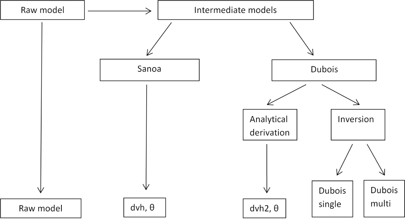
Figure 2 depicts the steps of our predictor selection procedure, the last row comprising of a total of five possible predictor groups. Dubois et al., (1995) highlight the importance of validity regions for various semi-empirical formulas and that observational parameters must lie within these regions to ensure feasible/optimal values [17]. For example, for the standard Dubois formula, the conditions are that k · h_RMS ≤ 2.5, θ ≥ 30^o, m ≤ 35% (recall k = 2π/λ). For the Casselman data-set, λ = 5.6 cm, and θ varied between 35° and 37°. Negative values of ε have no meaning. Yet, there is still no general mathematical or theoretical guarantee that ε_r is positive when inverting using these formulas, even when the validity constraints or the so-called “Dubois conditions” are satisfied.

3.4. Model Structure

A suite of statistical models were constructed by combining different covariates and sources of information (RS data, ground data, spatial correlation) to obtain best-fitting soil moisture predictions at observed and unobserved locations. There are various ways the data can be built in a statistical model. Due to limitations on the data, one may not be able to predict using all possible predictors and interaction terms; nonetheless, such a situation might lead to over-fitting, whereby, a statistical model performs very well for a training data set, but poorly for an independent set of validation data. Under-fitting can also occur when a significant influence on soil moisture is ignored. We consider two classes of models, namely: (1) models with only remotely-sensed covariates; and (2) models with both remotely-sensed and ground-based covariates. We compare results from applying these two class of models to investigate the predictive power and reliability of the remotely-sensed variables alone in predicting the soil moisture, and to investigate the relative improvement, benefit or gain in measuring ground-based variables.

We consider RS covariates, σ_vv, σ_hh, θ and the interaction terms θ × σ_vv, θ × σ_hh, which we denote as σ_vvθ, σ_hhθ. We also consider two other possible covariate forms, defined by,

$$dvh={\sigma }_{vv}-{\sigma }_{hh},$$

(14)

which is based on the recommendation of Sanoa et al., (1998) [25] and,

$$dv{h}_2=1.27{\sigma }_{vv}-{\sigma }_{hh}$$

(15)

which we have derived in reference to Equation (12). Note that in this Equation, the dielectric constant is only a function of dvh₂ and the incidence angle,

$$\epsilon ({\sigma }_{vv},{\sigma }_{hh},\theta ,h_{RMS})=f(dv{h}_2,\theta ),$$

(16)

Now, referring to Equation (13), soil moisture is a function (i.e., $h(\epsilon )=\sqrt{\epsilon }-1.6$) of the dielectric constant only, whereby soil moisture can be expressed as a function of σ_vv, σ_hh, θ and h_RMS, or, alternatively as a function g of dvh₂ and θ,

$$m({\sigma }_{vv},{\sigma }_{hh},\theta ,h_{RMS})=g(dv{h}_2,\theta ).$$

(17)

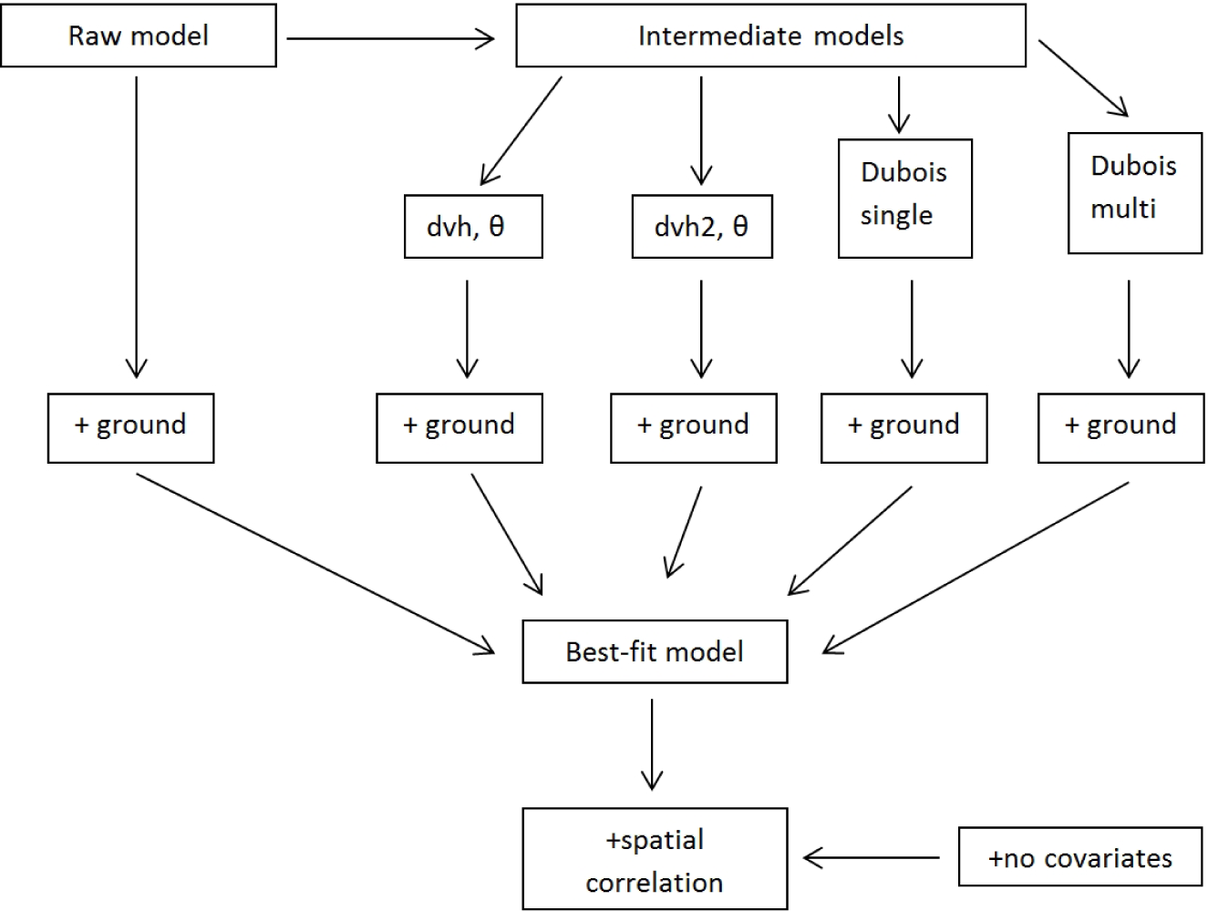
Hereafter, we refer to the variables dvh and dvh₂ as “intermediate” variables. We consider models using the dielectric constants, ε_r(hh), ε_r(vv), ε_r(hh,vv), obtained in Equations (10) to (12). For covariate selection, we first use the data at Times 1–3 separately and then consider all the time points combined. We modelled at each of the three acquisition times individually to determine the best models under variation in the ground-based sampling data and SAR configuration (e.g., incident angle), and to obtain independent estimates of model performance or prediction power across this observation time window. In this way, we compute cross-validation model error to isolate the best-fitting or “optimal” models. For the response, we can consider either the raw values of the soil moisture m, as a proportion, or its logit (Z(m) = log(m/(1 − m)). We note that there is very little difference in results obtained from analyses of m versus Z(m) and results presented here are based on m. This procedure that was applied (refer to flow diagram shown in Figure 3) to inter-compare the predictive power of competing statistical models and to select the best-fitting model consisted of several decision steps. At the highest layer, we selected the best model (in terms of prediction error as explained below) for each of the five model families; in the second layer we choose the best model for each of the families in conjunction with ground data; in the third layer, we choose the best of all the models over the families of models; and finally in the last layer we add spatial correlation.

Spatial models without any predictors were also considered (last decision layer). Note that the overall best model may not incorporate some elements, across all layers considered, for example the spatial models may not improve over a non-spatial model, despite involving the same set of predictors of soil moisture. This can be considered as a particular example of over-fitting as spatial models involve more parameters as compared to the corresponding non-spatial models. For each model, we have listed the associated unique family or set of covariates (refer to

Table 3. Table shows the covariates corresponding to every model family.

Model Family	Covariates
Raw	σvv, σhh, θ, σvvθ, σhhθ
Intermediate (dvh)	dvh, θ, dvhθ
Intermediate (dvh2)	dvh2, θ, dvh2θ
Dub. Single	εhh, εvv
Dub. Multi	εhh,vv

). The “Raw” family includes raw remotely-sensed covariates. The “Intermediate” dvh (suggested by [25]) and dvh₂ families utilize transformations on the raw covariates, recall dvh₂ is created by manipulating the Dubois Formulas as described above. Dubois Single-polarized (Dub. Single) and Multi-polarized (Dub. Multi) families utilize the Dubois Formulas and incorporate the Dubois-derived dielectric constants as covariates. Figure 2 summarizes the procedure we performed to obtain the five different families or sets of predictors.

3.5. Model for Spatial Dependence

For fitting the spatial models we used maximum likelihood and Bayesian hierarchical methods [27,28]. For the maximum likelihood method (fitted using the geoR package) the estimates of the spatial decay parameter (range parameter) were very unstable. This confirms the spatial decay parameters are weakly identifiable, as previously reported by Finely et al., (2008) [29]. The Bayesian approach (implemented in R) for implementing the spatial version of our statistical model that we employed circumvented this problem by prescribing informative priors or distributions on the range parameter.

3.6. Model Performance Statistics

The cross-validation root-mean-square error (CVE) and cross-validated correlation (CVR) were selected to compare the performance of the different statistical model structures, comprising different predictors, covariates, and spatial correlation assumptions, and were computed as follows. CVR² is termed the predictive squared correlation coefficient or leave-one-out cross-validated R² and also denoted as Q². A high CVR is a necessary but not a sufficient condition for a model to have a high predictive power (i.e., goodness of fit), because different CVR values may arise from training data sets with different sample size and spatial distributions. Thus, the CVR value should always be accompanied by descriptive statistics of the training data set used to compute it, such as CVE (also denoted RMSE) [30,32]. We computed both of these measures. While a high value of this validation statistic (CVR² > 0.5) is typically considered sufficient for proof of the high predictive ability of the model from internal cross-validation (i.e., a LOOCV procedure), low values do not necessarily indicate a sufficient reason to question the validity of a model, but relate more to the size and distribution of training data used for prediction. Cross-validation with an external (i.e., independent) set of training data can further improve the reliability of a model. However, while the calculation of CVR² by LOOCV validation is based on a well-known and accepted formula, its derivation from an external training or evaluation data set is not trivial and varies with available sample size [30]. For each site s_i, i = (1, ⋯, n) (n = 44), a leave-one-out cross-validation (LOOCV) was performed that involved excluding the data/mean values for a given site, s_i, and predicting the value at s_i, on an iterative basis so that each of the sites have been excluded once. We denote the predicted values as $\tilde{m}(s_i)$, and compute cross-validation statistics (CVE and CVR) according to,

$$CVE=\sqrt{{\displaystyle \sum _{i=1}^n{(m(s_i)-\tilde{m}(s_i))}^2}}/n,CVR=corr\left(\left(\begin{array}{c}m(s_1)\\ ⋮\\ m(s_n)\end{array}\right)\right),\left(\left(\begin{array}{c}\tilde{m}(s_1)\\ ⋮\\ \tilde{m}(s_n)\end{array}\right)\right),$$

(18)

where corr denotes correlation.

4. Results

4.1. Predictor Selection and Validity of Model Predictions

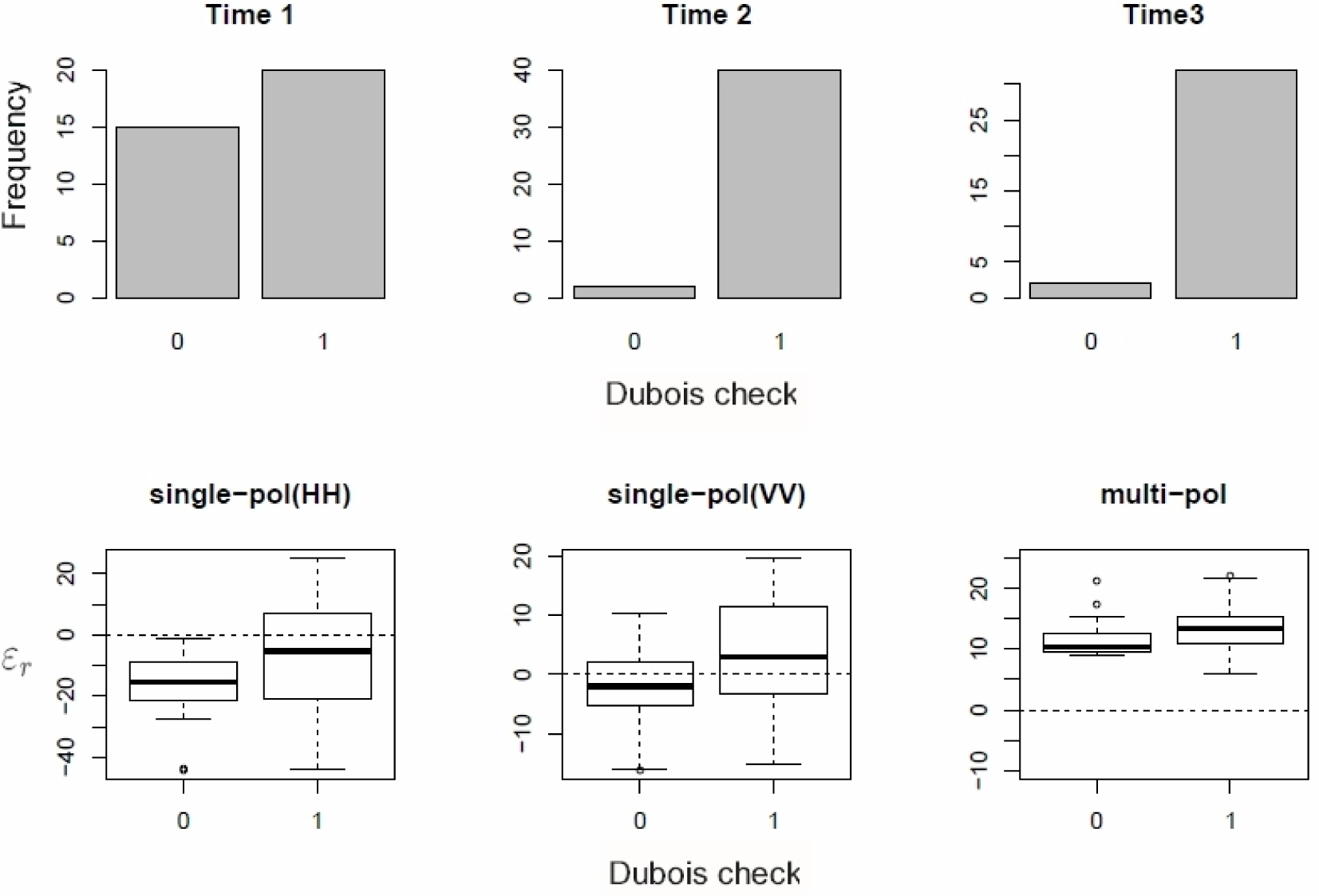
We have presented a set of competing statistical models having different covariates (i.e., the predictor variables). The simplest choice for a group of predictors is to use all the available raw RS variables and their interactions with each other. However, as the size of our data set is small (i.e., containing 44 total sampling points for three days) this choice may not necessarily be optimal due to potential over-fitting. In general, variable interactions may be non-linear and variable distributions, in different SAR soil moisture modeling applications could be directionally biased and/or highly skewed, possibly requiring different parameter and error distribution assumptions if tranformations applied do not approximate a normal or Gaussian statistical distribution (see Vereeken et al., (2014) for a detailed review of statistical features and dynamics of soil moisture patterns [23]). Figure 4 (top panels) show the frequency of the data points when the Dubois Conditions are satisfied (denoted by 1) versus when they are not satisfied (0), showing the Dubois validity conditions are not satisfied for a large proportion of measured values in the case of Time 1, but for the other Times 2 and 3, the conditions are satisified far more frequently. The bottom panels in Figure 4 depict the boxplot summaries of values of ε_r obtained from Dubois formulas: ε_r(hh), ε_r(vv), ε_r(hh,vv). We find that even for the data points for which the Dubois Conditions hold, ε_hh and ε_vv are negative for many of the data points. Contrary to this, for ε_r(hh,vv) all the values are positive, regardless of whether the Dubois Conditions are satisfied or not.

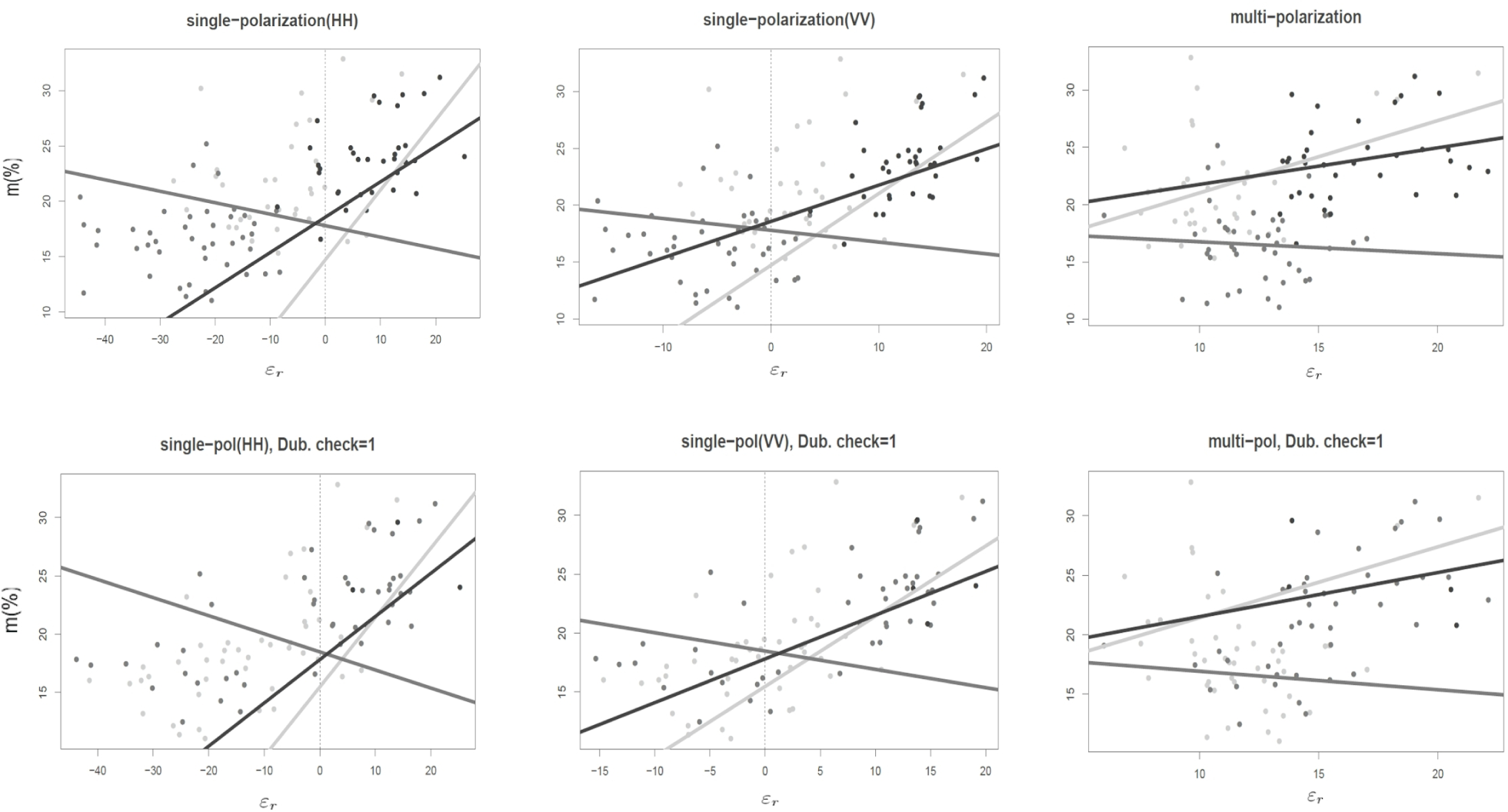
The relationship between the estimated dielectric constants, ε_r(hh), ε_r(vv), and ε_r(hh,vv), in comparison to estimated soil moisture is shown in Figure 5 (refer to top panels) for Time 1 (light grey), Time 2 (grey) and Time 3 (black). For each time, the corresponding simple regression line (relating m and ε) is provided in the corresponding color. The dotted line shows the vertical line ε = 0. It is clear that at Time 1 and Time 3 there is clear association between any of the estimated dielectric constants and the soil moisture. However at Time 2, when soil moisture estimates are consistently smaller, the relationship is weak and in the wrong direction (i.e., decreasing not increasing). Figure 5 further reveals that various associations of soil moisture with ε_r(hh), ε_r(vv) are stronger than ε_r(hh,vv). In the bottom panels, we have repeated the analysis with only the data points for which the Dubois Conditions are satisfied, and still the relationship is decreasing (negative), with no significant change and improvement to an increasing (positive) relationship.

Despite the limitations of using data from only one monitoring site and sampling data available only for three sampling days, a large change in the proportion of sampling data that satisfies validity conditions is evident. This highlights that caution must be taken when applying the Dubois or even other empirical-based formulae with fixed interval validity conditions. Instead of using or extending fixed validity assumptions and constraints imposed by empirical models, our statistical modeling approach offers the key important advantage that it is not constrained to any specific validity region, and avoids the need to independently discriminate and verify at what locations and at what times such conditions are met.

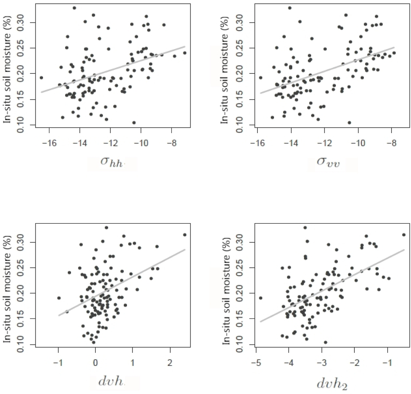
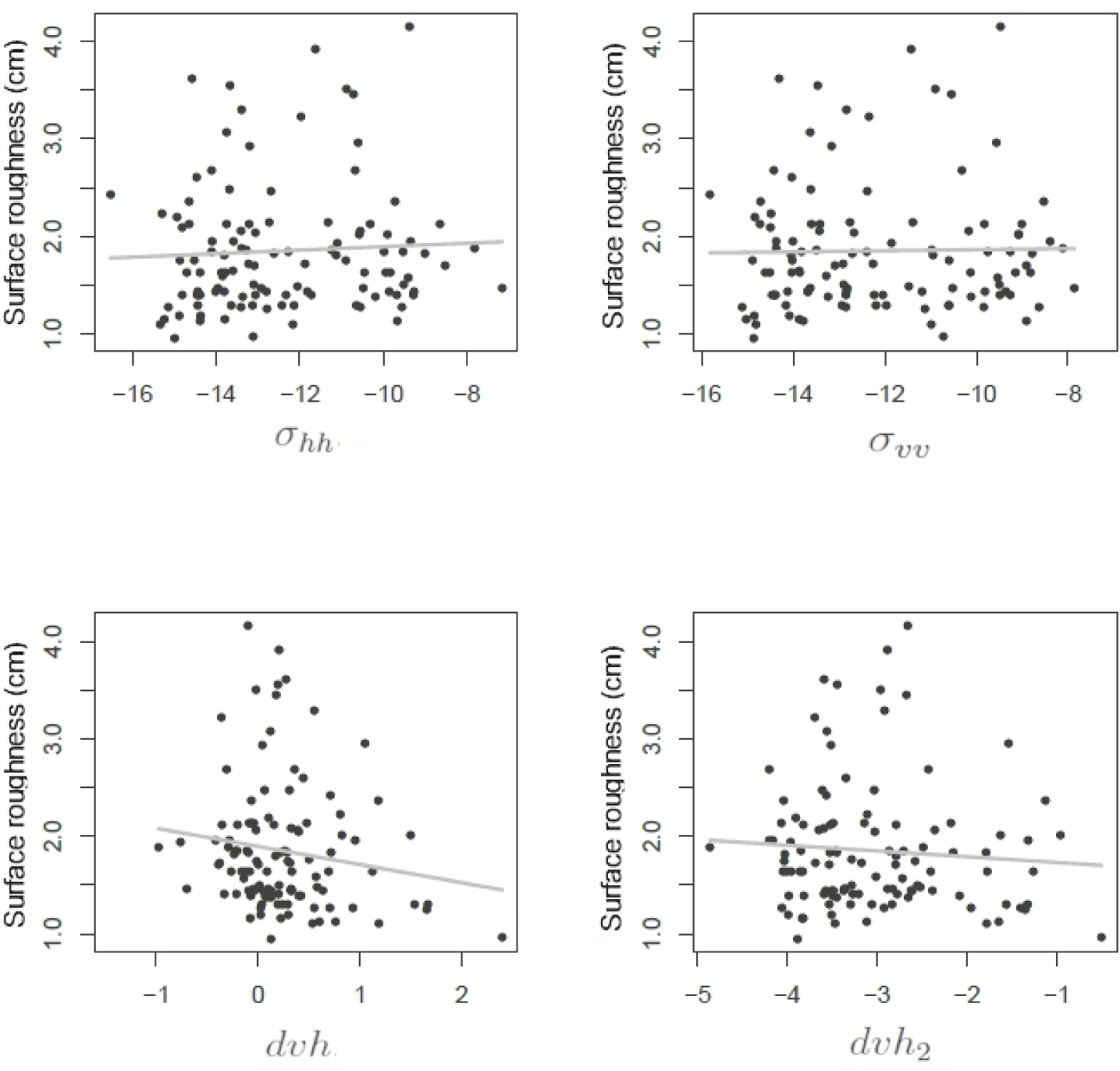
Figure 6 shows scatterplots of the backscatter coefficients (σ_hh, σ_vv) and the derived variables (dvh, dvh₂) with in-situ soil moisture (%), along with the regression line using the data from all three times. These results show a positive association between soil moisture and the predictors. Computed correlation (%) between each of these variables with both soil moisture (m) and surface roughness (i.e., root-mean-square height, h_RMS), for Times 1–3 and all the Times pooled are summarized in

Table 4. Correlation (%) between in-situ soil moisture (m)(%) and surface roughness (h_RMS) (cm) with the four leading model predictors (σ_vv, σ_hh, dvh, dvh₂), respectively. Uncertainty in these correlation estimates was estimated from standard statistical bootstrapping based on 1000 bootstrap samples. The 10th, 50th (median) and 90th quantiles are indicated, respectively, with the median values highlighted in bold.

(m, Predictors)	Time 1	Time 2	Time 3	Pooled (Times 1–3)
σvv	−9, 16, 40	−39, −18, 4	2, 24, 42	37, 47, 56
σhh	−19, −1, 21	−37, −18, 4	−6, 12, 32	30, 40, 49
dvh	30, 43, 55	−11, −3, 6	4, 13, 23	34, 40, 45
dvh2	26, 41, 52	−19, −13, 2	14, 24, 34	51, 55, 60
(hRMS, Predictors)	Time 1	Time 2	Time 3	Pooled (Times 1–3)
σvv	9, 34, 55	−24, −5, 16	1, 24, 46	−11, 1, 12
σhh	24, 47, 64	−13, 6, 26	1, 22, 41	−6, 6, 17
dvh	−45, −30, −9	−56, −44, −30	−27, −5, 19	−24, −15, −5
dvh2	−26, −3, 31	−48, −33, −14	−21, 3, 25	−18, −8, 2

. Uncertainty in the correlation values are based on standard statistical bootstrapping method based on the 10th, 50th (median) and 90th quantiles and 1000 bootstrap samples. These results indicate that dvh and dvh₂ both have a positive and significant association (i.e., with respect to percent bootstrap confidence interval) with soil moisture at Times 1 and 3 and all three Times pooled, while σ_vv and σ_hh have higher uncertainty and their confidence intervals include zero. At Time 2 we do not observe significantly positive correlation between soil moisture and any of the predictors. When pooling our data across all three Times, the largest correlation is obtained between soil moisture and dvh₂. Scatterplots of the backscatter coefficients (σ_hh,σ_vv) and the derived variables (dvh, dvh₂) with h_RMS are shown in Figure 7, with correlation values summarized in Table 4. The variable h_RMS is positively correlated with the two predictors, σ_hh and σ_vv at Times 1 and 3, with the 80% confidence interval indicating that such association is significant. For the derived variable, dvh₂, a non-significant correlation is evident at Times 1 and 3, while for both dvh, and dvh2 at Time 2 there is significant negative correlation. A non-significant correlation of a variable with h_RMS is desirable for the form of models which use dvh₂ as a predictor, but do not explicitly include h_RMS. According to this criterion, dvh₂ is the most desirable predictor for models that do not include h_RMS as a variable at Times 1 and 3.

4.2. Performance of Different Statistical Model Structures

Model validation/performance measures (i.e., cross-validation root-mean-square-error, CVE, and cross-validated correlation, CVR) for different statistical model structures (i.e., families) are summarized in

Table 5. Model selection for soil moisture estimation on the ground at Time 1 (5 Time 2 (16 May) and Time 3 (23 May). CVE in the table stands for the mean cross-validation error and CVR stands for cross-validated correlation. The best for each time point is denoted by a star.

	Model Family (Time 1)	Best Model	CVE (%)	CVR
(Remote only)	Raw	σvv, σhhθ	4.4٭	0.31
	Interm. (dvh)	dvh, θ	4.4٭	0.33
	Interm. (dvh2)	dvh2, dvh2θ	4.4٭	0.29
	Dub. Single	εhh, εvv	4.6	0.19
	Dub. Multi	εhh,vv	4.5	0.27
(+ ground)	Only ground	ST, CL	4.5	0.29
	Raw + ground	σvv, σhhθ, CL	4.3	0.38
	Interm. (dvh) + ground	dvh, ST, CL	4.3	0.40
	Interm. (dvh2) + ground	θ, dvh2, dvh2θ, CL	4.2٭	0.43
	Dub. Single + ground	εhh, εvv, CL	4.4	0.34
	Dub. Multi + ground	εhh,vv, CL	4.3	0.39
	Model Family (Time 2)	Best Model	CVE (%)	CVR
(Remote only)	Raw	θ	3.2٭	−0.02
	Interm. (dvh)	θ	3.2٭	−0.02
	Interm. (dvh2)	θ	3.2٭	−0.02
	Dub. Single	εhh	3.3	−0.73
	Dub. Multi	εhh,vv	3.3	−0.49
(+ ground)	Only ground	none	3.3	−1.00
	Raw + ground	θ	3.2٭	−0.02
	Interm. (dvh) + ground	θ	3.2٭	−0.02
	Interm. (dvh2) + ground	θ	3.2٭	−0.02
	Dub. Single + ground	εhh, ST	3.3	−0.08
	Dub. Multi + ground	εhh,vv	3.3	−0.49
	Model Family (Time 3)	Best Model	CVE (%)	CVR
(Remote only)	Raw	θ	3.3	0.27
	Interm. (dvh)	θ	3.3	0.27
	Interm. (dvh2)	θ	3.3	0.27
	Dub. Single	εhh, εvv	3.0٭	0.47
	Dub. Multi	εhh,vv	3.5	0.03
(+ ground)	Only ground	hRMS, ST	3.3	0.31
	Raw + ground	σ vv, σvvθ, σhhθ, ST, CL	2.8٭	0.58
	Interm. (dvh) + ground	θ, ST, CL	2.9	0.56
	Interm. (dvh2) + ground	dvh2, dvh2θ, ST, CL	2.8٭	0.59
	Dub. Single + ground	εhh, εvv, ST	2.8٭	0.56
	Dub. Multi + ground	εhh,vv, hRMS, ST	3.0	0.49

. Different model families are identified according to the two groups we considered: (1) models that only include remotely-sensed covariates (remote only) and (2) models that include both remotely-sensed and ground-based variables (+ ground). For each model family, models with all the possible combinations of corresponding covariates are fitted and the best model is identified as having the smallest mean squared cross-validation error. At both Times 1 and 3, models involving dvh₂ are among the best models and adding ground covariates has turned out to be useful with CL appearing in the best models at both times. At Time 2 there are no satisfactory models and the best models only include the incidence angle θ (which clearly cannot have any prediction power on its own).

Table 6. Model selection integrated data across all three observational days. The best model(s) in terms of CVE, is (are) denoted by a star.

	Model Family	Best Model	CVE (%)	CVR
(Remote only)	Raw	σvv, σhh, σvvθ, σhhθ	3.8	0.64
	Interm. (dvh)	θ, dvh, dvhθ	3.7٭	0.65
	Interm. (dvh2)	θ, dvh2, dvh2θ	3.7٭	0.65
	Dub. Single	εvv	3.9	0.60
	Dub. Multi	εhh,vv	4.6	0.32
(+ ground)	Only ground	none	5.0	0.08
	Raw + ground	σvv, σhhθ, CL	3.7٭	0.64
	Interm. (dvh) + ground	θ, dvh, dvhθ, CL	3.7٭	0.65
	Interm. (dvh2) + ground	θ, dvh2, dvh2θ, hRMS, CL	3.7٭	0.65
	Dub. Single + ground	εvv, hRMS, CL	3.9	0.61
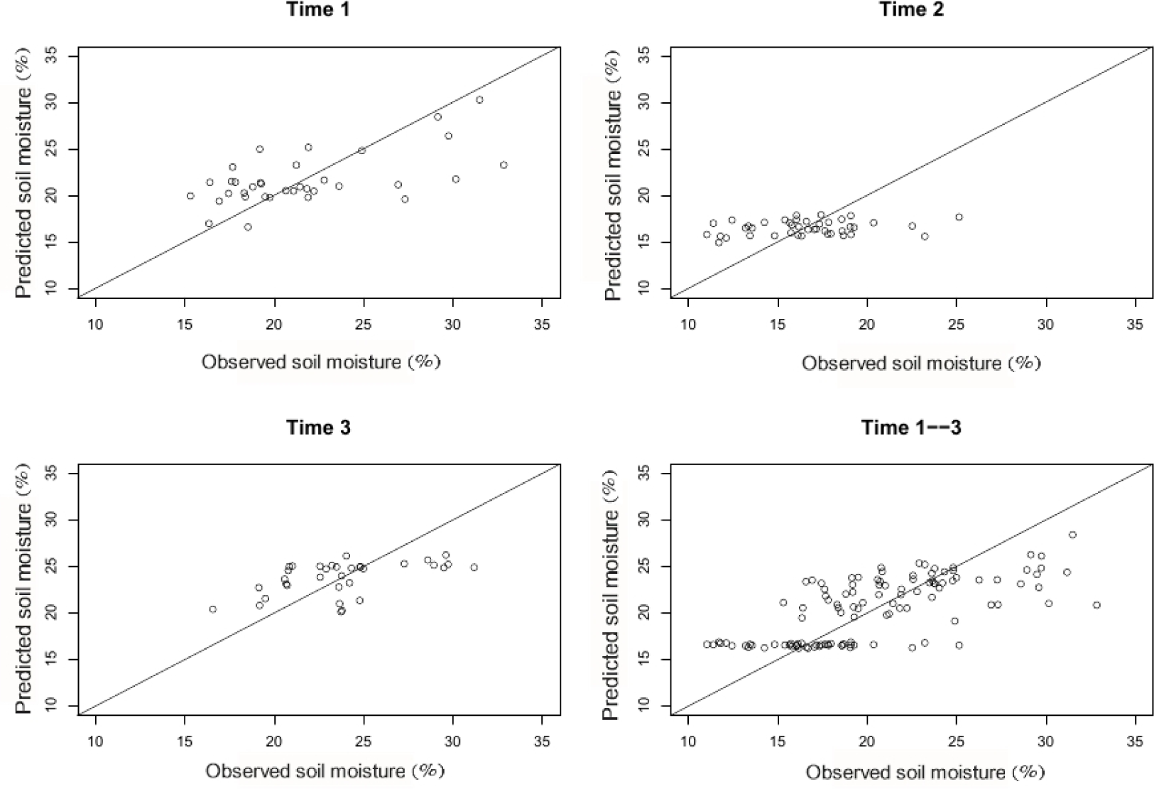
	Dub. Multi + ground	εhh,vv, CL	4.6	0.35

summarizes our results for the same covariate selection procedure, but now applied to the data pooled together across all the three times. In this case, we forced the categorical time covariate (Time 1, 2 or 3) to be a covariate in the model. This is because soil moisture varies across time and this prevents artificially selecting covariates that are confounded with time such as θ. In this case, models including dvh₂ are again among best models. However, adding the ground covariates did not improve the prediction of the soil moisture. The leave-one-out cross-validation (LOOCV) results are shown in comparison to observed data in Figure 8. For each model and data point, we take the data point out, fit the model and then predict the point which was taken out. In each panel, the LOOCV prediction is plotted against the observed value. The cross-validation correlation includes more than just the correlation between model predictions/fitted values and the full set of observations in evaluating prediction power or model performance, and a relatively high correlation indicates reasonable model performance in relation to observed inter-site variability. The results indicate that the fit at Time 2 is far from satisfactory for multi-site prediction. The top right panel shows that the predicted values at Time 2 fail to capture the increase of soil moisture on the x-axis. Also, in the bottom right plot, we note that the clustering of data along a line segment which sits below the rest of the data can be attributed to the inclusion of data from Time 2. The standard deviations (SD’s) in observed soil moisture across all sites for Time 1, 2 and 3 are 5.1, 3.3, 4.1, respectively. Comparing these estimates with the best model CVE’s (i.e., 4.2, 3.2, 2.8, respectively), indicates that a significant portion of the observed variation in soil moisture is explained by the models at Times 1 and 3, but less so at Time 2.

4.3. Influence of Spatial Correlation

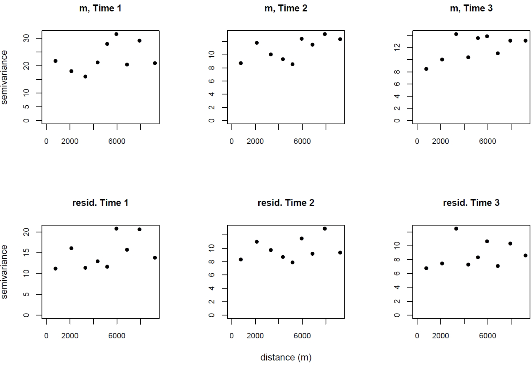
The spatial correlation of soil moisture can potentially help us improve the predictions of soil moisture across space and is considered in this context in [10,11,14]. We summarize statistical model predictions obtained from including spatial correlation in the various statistical models developed here. The top panels of Figure 9 depict the semivariogram (created by geoR package, [33]) for the raw soil moisture data, while the bottom panels depict the semivariogram for the residuals after fitting the best models at each time point. In the presence of strong spatial correlation, semivariance increases with the separation distance between the location of pairwise observation measurements. Both the raw data and the remaining noise confirm this increasing trend, but the signal for the spatial correlation is weak. A summary of results obtained from fitting the spatial models to data, both with and without predictors is provided in

Table 7. Model validation statistics, comparing the relative performance of the best-fitting spatial versus non-spatial models. The best model(s) in terms of CVE, is (are) denoted by a star.

Time	Model	CVE (%)	CVR
Time 1	spatial, no cov.	4.9	−0.09
	spatial, with cov.	4.8	0.26
	best non-spatial	4.2٭	0.43
Time 2	spatial, no cov.	2.9٭	0.25
	spatial, with cov.	3.0	0.25
	best non-spatial	3.2	−0.02
Time 3	spatial, no cov.	3.8	−0.11
	spatial, with cov.	3.2	0.45
	best non-spatial	2.8٭	0.59

. The corresponding non-spatial fits are also included for comparison purposes. We considered isotropic spatial covariance functions of the exponential and Matérn form as discussed in [34].

Given that we have a small sample size and the weakness of the spatial influence detected in the current data-set, non-isotopic spatial functions were not considered. This does not, however, rule out the possibility that the spatial influence might be stronger given more data for the Casselman site, or for data on other agricultural monitoring sites. So, spatial influences can be prominent, even if weak in our current data set, and modeling needs to be flexible in detecting this changing influence across different sampling sites. Only small deviations were detected between specifying an exponential versus a Matérn covariance function (results not shown here), and therefore we only include results for the exponential covariance function that did reveal significant influences in model prediction. Our numerical results also reveal that the spatial models only improved the CVE in the case of Time 2, the same time when predictors also did not show any prediction power in non-spatial models.

5. Discussion

Our findings demonstrate how semi-empirical models and their assumptions may not be satisfied in a large proportion of data, and furthermore, even when the conditions are satisfied, the dielectric constant using single-polarization method, often can lead to negative i.e., nonsensical soil moisture predictions. Such negative values did not result when employing the multi-polarization method however. Single-polarization values, even when negative, generated predicted patterns of soil moisture having strong correlation with observations (Figure 5). Statistical models do not suffer from these validity constraints and performance statistics that they generate provide a more sound assessment of their reliability to be applied to other regions and application contexts, than deterministic models. Prediction error (root mean square error, RMSE) from previous work that has applied the Dubois multi-polarization method is estimated at 6.2% [14]. With our statistical modeling approach, the best-performing model offers a significant improvement (i.e., a significant reduction of prediction error) within the range of 3%–4%.

Data in this modeling study was available at three time points (Time 1–Time 3) during the early weeks of the crop growing season in 2008; 5 May (Time 1), 16 May (Time 2) and 23 May (Time 3). We evaluated and compared a selected set of statistical models that do not include any ground-based covariates that are typically measured (soil type, h_RMS, CL). The first three rows of Table 3, correspond to three model families which do not depend on ground variables. In particular models including dvh and dvh₂ are constructed so that the effect of h_RMS (a ground variable) is included through other variables and direct values for this observation are not needed. We investigated whether the ground covariates can improve the predictions of these models by adding ground variables to each family. The predictions were improved for models in Time 1 and Time 3, but did not improve for Time 2. Also the best models in terms of prediction for the data combined across the three times included models with no ground predictors. For Time 1 and Time 3, models involving dvh₂ = 10 log₁₀ ((σ^vv)^1.27/σ^hh) (Dubois), were among the best models; including ground covariates such as CL improved the prediction accuracy. However for Time 2, the prediction was not satisfactory in any of the non-spatial models. Two differences between Time 2 and Times 1, 3 are the smaller incidence angle and smaller soil moisture values and spatial variability. Rainfall, evapotranspiration would be expected to induce larger differences, so that we infer that the reason why spatial dependence was detected at Time 2 was likely due to sufficiently dry conditions that made it more difficult to discriminate soil moisture variability using SAR. As indicated by Merzouki et al., (2011) in conjunction with processing and analysis of the same SAR acquisition and Casselman ground-based data, a significant accumulation of precipitation preceded the first acquisition, followed by relatively little precipitation between this acquisition and the second acquisition of 16 May. In addition, warm day time temperature aided in the drying of the top soil prior to 16 May [14]. A relatively high error in the field measurement of correlation length (CL) was likely the result of its sensitivity to profile length [35]. As outlined by Merzouki et al., (2011), relatively short lengths (1 m) were used. A much longer profile length (i.e., >10 m) might have reduced the high nugget variance, but contrasting results are reported in the literature. Also, in obtaining the current data set, shorter length was used, in part, due to practical considerations and constraints of time, labour and cost [14].

Overfitting of statistical predictions can occur when a statistical model is fit to training data but provides poor prediction using an independent data set [36]. The solution to this problem is not to include all possible covariates into the model and to detect as much variability and signal information in a given data set. This requires variable and model selection statistical techniques. Existing methods to handle and control overfitting can be organized into three categories [36]: (1) iterative selection methods (such as step-wise regression); (2) regularization methods such as Least Absolute Shrinkage and Selection Operator (Lasso), or, (3) statistical averaging methods (such as Bayesian model averaging) [37]. In this paper, we utilized the first of these approaches, devising a grouped, stepwise method that conducts an iterative search of the predictor space corresponding to a group of selected leading predictors. This extends regular stepwise methods to the multivariate case [38–40]. A widely used measure in validating soil moisture estimation algorithms in the literature is the Root Mean Squared Error (RMSE) [7,14]. Despite its popularity, this measure does not deal with over-fitting problems and can lead to eronous conclusions. Instead, alternative validation measures have been developed, namely: Akaike Information Criterion (AIC) [41], the Bayesian Information Criterion (BIC) [42] and Deviance Information Criterion (DIC) [43]. These are termed likelihood-based measures and assess overfitting, but cross-validated RMSE (CVE) and correlation (CVR) provide a measure of accuracy of predictions of a model. CVR showed more deviation and was more responsive than CVE. Possible multi-collinearity effects may need to be considered in our modeling arising from sampling points that are sufficiently close together in areas that show reduced soil moisture variability. Depending on the sites selection and their spacing arrangement, spatial correlation may be informative, because very close sites may have a stronger tendency to exhibit similar soil moisture variability. In contrast, sampling a very large area more sparsely may only capture some variations, but not all, within a full sampling extent. Higher deviations in the performance of different models would be expected for other sampling regions under different soil, climate, crop, and landscape variation. A small deviation in CVE and CVR can lead to large spatial uncertainty and error when propagated spatially and temporally (i.e., interpolation and extrapolation). Nonetheless, to capture observed daily, weekly, monthly variability in soil moisture more comprehensively, requires data across a larger time interval and number of acquisition dates. This would enable temporal components of soil moisture variability to be added to the statistical models and involved in the multivariate regressions.

Soil moisture variability at the our study site may, at certain times, be very spatially homogeneous, such that a more heterogeneous region (e.g., in terms of surface roughness, soil variation etc.) would be best for training and validating a statistical modeling approach. Li and Rodell (2013) have recently highlighted how soil moisture is often sampled over a short time period and this results in the observed soil moisture often exhibiting smaller dynamic ranges that prevents unravelling soil moisture spatial variability as a function of mean soil moisture [44]. They also provide evidence of power-law scaling in soil moisture variability driven by climate variables such as rainfall. They log-transform soil moisture values, and this might further help to improve the detection of soil moisture variability within our statistical modeling, especially at times when soil moisture variability is reduced. Our analysis identifies that one of these differences may be the reason for the poor prediction power. At Time 2 spatial correlation improved prediction accuracy (i.e., reduced model prediction error), while at Time 1 and Time 3 with weak spatial correlation, including spatial correlation did not improve prediction accuracy. At Time 2, the covariates did not show any prediction power, while the spatial model offered minor improvement and captured a greater portion of the observed variability in soil moisture. As the CVR statistic is sensitive to the sample size of our training set and its spatial distribution, higher predictive power (i.e., higher CVR) could be achieved with training data that has a higher variability in soil moisture than our training data set (e.g., at Time 3 where the value of CVR² was 0.35 < 0.50). The standard deviations (SD’s) in observed soil moisture across all sites for Times 1, 2 and 3 are 5.1%, 3.3%, 4.1%, respectively. Such low spatial variability of soil moisture makes training statistical models, assessing and interpreting their predictive performance more challenging. Comparing such observed variability with the best-model CVE estimates (i.e., 4.2%, 3.2%, 2.8% for Times 1, 2 and 3, respectively), indicates that the best models at Time 1 and 3 explain a portion of the observed spatial variability of the soil moisture, despite low observed variation in the training data set. The lower predictive performance at Time 2 may be due, in part, to the very low observed SD (i.e., 3.2%), as well as, the small incidence angle. As our results show, the pooling of data/acquisitions across times of high variability may also be necessary to sufficiently increase model predictive power.

Our results show that when integrating ground-based soil moisture data as auxiliary data with SAR remote-sensing data for model prediction (i.e., not just estimation) to achieve high predictive power from statistical models, requires a sufficiently large set of training data and spatially heterogeneous regional variability. Our findings support those of Van der Heijden et al., (2007) who have also previously determined that in remote-sensing across agricultural land, the predictive performance of statistical models is under-estimated with the CVR statistic, given its high sensitivity to the degree of spatial heterogeneity and size of the training data set used in LOOCV cross-validation [45]. SAR analyses and modeling studies vary substantially in terms of the quantity and quality of data they rely on - some reported studies utilize data collected during 2–3 months during a growing season while others have monitoring a region for up to 6 years. The number and interval of SAR acquisitions also substantially varies (e.g., 2–11 images), including the number and distribution of sampling sites (e.g., 5–50), often with very limited within-site sampling to enable a reliable determination of intra-site variance. Many SAR analysis and modeling studies have relied on coefficient of determination (i.e., R²) statistics, and in some cases, considering R² = 0.30 (i.e., instead of 0.50 or larger values) as the threshold criteria for accepting a given model for reliable estimation and/or prediction. While there is currently no broad consensus on the acceptable threshold for soil moisture prediction, as our findings show, by relying on additional cross-validated statistics, the reliability of a model can be better gauged in terms of its ability to attain prediction-based targets, thresholds and criteria. The inter-comparison of a broader set of such statistics could also help to limit additional bias introduced in the under and over-estimation of soil moisture extremes in SAR analyses, especially when predictions rely on sampling distributions, rather than more complete statistical distribution/moments information. Data availability, costs and coverage are often an area of trade-off that challenges many SAR analyses and modeling studies, so “stress-testing” models and their predictive power, as in this study, under situations of high data sparsity and high variability provides a realistic, operational situation that many practitioners and scientists confront.

6. Conclusions

In this study, we demonstrated a statistical modeling approach for improving the robustness of soil moisture predictions. We quantifed and inter-compared the predictive power of different models and variables for predicting soil moisture. This approach offers a way to consider a broad set of spatio-temporal assumptions required to identify, select, and validate alternative, competing models, predictors, covariates and spatial correlation assumptions. The approach also does not impose any rigid a priori validity bounds on its inputs, nor overriding fixed constraints in its output predictions, as is the case with many existing soil moisture retrieval methods. Leave-one-out cross-validation (LOOCV) is also integrated. We applied our approach to an agricultural region in Canada with available C-band, multi-polarization SAR data with multi-site ground-based data. Under non-ideal SAR monitoring conditions, employing both model- and predictor-based selection steps, we obtained a best-performing model with a significant reduction of prediction error to within 3%–4%. We found that ground-based data are useful for improving soil moisture prediction, but not in all situations, such as when climate conditions are highly variable, landscape is too homogeneous and/or spatial correlation of soil moisture is low. We further determined that the cross-validated statistic, CVR², was more sensitive than CVE². Our study was limited, however, by available data, namely; one study site, only three SAR acquisitions (i.e., images), and a limited range of surface roughness and soil moisture variability. In addition, high error in correlation length from the use of shorter profile length measurements was also a limitation in the data used to train the models.

The Dubois model was selected in our study as it has a mathematical closed-form solution that enables eliminating the surface roughness parameter (h_RMS) so that a closed-form equation could be derived for the reflectivity, and distinguishing two “model families”—one that includes h_RMS as a predictor and another that does not. The use of the Dubois model also enabled highlighting numerical issues with using empirical-based equations having validity constraints when coupling them within a generalized (i.e., broader and integrated) statistical-based approach. Currently, a lower sensitivity and early saturation reported for the IEM model to soil moisture under wet conditions (i.e., extreme soil moisture) indicates that there are significant challenges faced by both simpler and more complex retrieval models in estimating and predicting soil moisture under wet conditions and at the regional-scale of variability [46]. Our study utilized predictors that depend on/are linked with the Dubois equations, but also included predictors linked with a “Raw model” and “Sanoa model” branch that do not dependent on the Dubois equations. Each of these model families included many models that were compared with or without ground data and spatial correlation. By including the Oh, or the more complex IEM models into our approach, it may be possible to further reduce prediction error, and to expand its potential application and usefulness.

There are increasing demands for greater predictive power and reliability in model-based predictions. Such information can be used in commodity market forecasting and price adjustments, setting risk insurance coverage and premiums associated with extreme events (e.g., droughts, floods) affecting crops across large agricultural regions, or for geospatial intelligence and planning for early-warning disaster response. For this reason, there is a great need for a consistent methodology, which can be further adapted and tuned to integrate across data sets, models and assumptions, for generating cross-validated soil moisture predictions in an reliable and rapid (automated) way. In the future, statistical-based modeling of very large amounts of RS data on soil moisture will also be increasingly important for integrating data that is multi-scale (i.e., coarse and fine-scale) data and to increase predictive power across a wide range of monitoring conditions and constraints. To help advance soil moisture studies for model-based prediction, NASA’s Soil Moisture Active Passive (SMAP) mission was just successfully launched on 31 January 2015 SMAP Mission. SMAP has on-board a synthetic aperture radar (active) instrument operating with multiple polarizations, not in C-band like RADARSAT-2, but in the L-band range (1.20–1.41 GHz). It integrates active and passive sensors for coincident fine-scale SAR and coarser-scale measurements (9 km footprints) for producing global soil moisture maps every three days. As a way forward—the approach we have presented in this study, with further enhancement and improvement, could provide the consistent and reliable approach needed to integrate different models, predictors, covariates and spatio-temporal correlation assumptions using SMAP SAR data obtained under a wide range of climate, landscape, soil, crop conditions. In addition, linking our approach across additional agricultural regions with ground-based data remotely-streamed from wireless sensor network-based monitoring technology may provide an efficient and strategic way to obtain internal (i.e., training) and external validation data. Such technology provides semi-continuous soil moisture sampling with automated data processing that can help to further increase the usefulness and reliability of our statistical modeling approach in predicting soil moisture to aid in regional-scale decision-making [47].

References

- Gao, G. Statistical modeling of SAR images: A survey. Sensors 2010, 10, 775–795. [Google Scholar]
- Ouchi, K. Recent trend and advance of synthetic aperture radar with selected topics. Remote Sens. 2013, 5, 716–807. [Google Scholar]
- Romano, N. Soil moisture at local scale: Measurements and simulations. J. Hydrol. 2014, 516, 6–20. [Google Scholar]
- Pratola, C.; Barrett, B.; Gruber, A.; Kiely, G.; Dwyer, E. Evaluation of a global soil moisture product from finer spatial resolution SAR data and ground measurements at Irish Sites. Remote Sens. 2014, 6, 8190–8219. [Google Scholar]
- Shi, J.; Wang, J.; Hsu, A. Y.; O’Neill, P. E.; Engman, E. T. Estimation of bare surface soil moisture and surface roughness parameter using L-band SAR image data. IEEE Trans. Geosci. Remote Sens. 1997, 35, 1254–1266. [Google Scholar]
- Stein, A.; Bastiaanssen, W.G.M.; De Bruin, S.; Cracknell, A.P.; Curran, P.J.; Fabbri, A.G.; Gorte, B.G.H.; van Groenigen, J.W.; van Der Meer, F.D.; Saldana, A. Integrating spatial statistics and remote sensing. Int. J. Remote Sens. 1998, 19, 1793–1814. [Google Scholar]
- Lakhankar, T.; Ghedira, H.; Temimi, M.; Sengupta, M.; Khanbilvardi, R.; Blake, R. Non-parametric methods for soil moisture retrieval from satellite remote sensing data. Remote Sens. 2009, 1, 3–21. [Google Scholar]
- Geng, H.; Hugh, Q.; Gwyn, J.; Brisco, B.; Boisvert, J.; Brown, R. Mapping of soil moisture from C-Band radar images. Can. J. Remote Sens. 1996, 22, 117–126. [Google Scholar]
- Quesney, A.; Hégarat-Mascle, S.L.; Taconet, O.; Vidal-Madjar, D.; Wigneron, J.P.; Loumagne, C.; Normand, M. Estimation of watershed soil moisture index from ERSSAR data. Remote Sens. Environ. 2000, 72, 290–303. [Google Scholar]
- Glenn, N.F.; Carr, J.R. The use of geostatistics in relating soil moisture to RADARSAT-1 SAR data obtained over the Great Basin, Nevada, USA. Comput. Geosci. 2003, 29, 577–586. [Google Scholar]
- Meade, N.; Hinzman, L.; Kane, D. Spatial estimation of soil moisture using synthetic aperture radar in Alaska. Adv. Space Res. 1999, 24, 935–940. [Google Scholar]
- Pultz, T.; Leconte, R.; Brown, R.; Brisco, B. Quantitative soil moisture extraction from airborne SAR data. Can. J. Remote Sens. 1990, 16, 56–62. [Google Scholar]
- Adams, J.R.; Berg, A.A.; McNairn, H.; Merzouki, A. Sensitivity of C-band SAR polarimetric variables to unvegetated agricultural fields. Can. J. Remote Sens. 2013, 39, 1–16. [Google Scholar]
- Merzouki, A.; McNairn, H.; Pacheco, A. Mapping soil moisture using RADARSAT-2 data and local autocorrelation statistics. IEEE J. Sel. Top. Appl. Earth Obs. Remote Sens. 2011, 4, 128–137. [Google Scholar]
- Zribi, M.; Chahbi, A.; Lili Chabaane, Z.; Duchemin, B.; Baghdadi, N.; Amri, R.; Chehbouni, A. Soil surface moisture estimation over a semi-arid region using ENVISAT ASAR radar data for soil evaporation evaluation. Hydrol. Earth Syst. Sci. 2011, 15, 345–358. [Google Scholar]
- Paloscia, S.; Pampaloni, P.; Pettinato, S.; Santi, E. A comparison of algorithms for retrieving soil moisture from ENVISAT/ASAR images. IEEE Trans. Geosci. Remote Sens. 2008, 46, 3274–3284. [Google Scholar]
- Dubois, P.C.; van Zyl, J.; Engman, T. Measuring soil moisture with imaging radars. IEEE Trans. Geosci. Remote Sens. 1995, 33, 915–926. [Google Scholar]
- Oh, Y.; Sarabandi, K.; Ulaby, F.T. Semi-empirical model of the ensemble averaged differential mueller matrix for microwave backscattering from bare soil surfaces. IEEE Trans. Geosci. Remote Sens. 2002, 40, 1348–1355. [Google Scholar]
- Bryant, R.; Moran, M.S.; Thoma, D.P.; Holifield Collins, C.D.; Collins; Skirvin, S.; Rahman, M.; Slocum, K.; Starks, P.; Bosch, D.; et al. Measuring surface roughness height to parameterize radar backscatter models for retrieval of surface soil moisture. IEEE Geosci. Remote Sens. Lett. 2007, 4, 137–141. [Google Scholar]
- Baghdadi, N.; Abou-Chayya, J.; Zribi, M. Semi-empirical calibration of the Integral Equation Model for SAR data in C-band and cross polarization using radar images and field measurements. IEEE Geosci. Remote Sens. Lett. 2011, 8, 14–18. [Google Scholar]
- Baghdadi, N.; King, C.; Chanzy, A.; Wigneron, J.P. An empirical calibration of the integral equation model based on SAR data, soil moisture and surface roughness measurement over bare soils. Int. J. Remote Sens. 2002, 23, 4325–4340. [Google Scholar]
- Rahman, M.M.; Moran, M.S.; Thoma, D.P.; Bryant, R.; Holifield Collins, C.D.; Jackson, T.; Orr, B.J.; Tischler, M. Mapping surface roughness and soil moisture using multi-angle radar imagery without ancillary data. Remote Sens. Environ. 2008, 112, 391–402. [Google Scholar]
- Vereecken, H.; Huisman, J.A.; Pachepsky, Y.; Montzka, C.; van der Kruk, J.; Bogena, H.; Weihermuller, L.; Herbst, M.; Martinez, G.; Vanderborght, J. On the spatial-temporal dynamics of soil moisture at the field scale. J. Hydrol. 2014, 516, 76–96. [Google Scholar]
- Gadelmawla, E.S.; Koura, M.M.; Maksoud, T.M.A.; Elewa, I.M.; Soliman, H.H. Roughness parameters. J. Mater. Process. Techn. 2002, 123, 133–145. [Google Scholar]
- Sanoa, E.E.; Moran, M.S.; Huetea, A.R.; Miura, T. C and multi-angle Ku-Band synthetic aperture radar data for bare soil moisture estimation in agricultural areas. Remote Sens. Environ. 1998, 64, 77–90. [Google Scholar]
- Srivastava, H.S.; Patel, P.; Manchanda, M.L.; Adiga, S. Use of multi-incidence angle RADARSAT-1 SAR data to incorporate the effect of surface roughness in soil moisture estimation. IEEE Trans. Geosci. Remote Sens. 2003, 41, 1638–1640. [Google Scholar]
- Diggle, P.J.; Ribeiro, P.J. Model-Based Geostatistics; Springer: New York, NY, USA, 2007. [Google Scholar]
- Banerjee, S.; Gelfand, A.E.; Carlin, B.P. Hierarchical Modeling and Analysis for Spatial Data; CRC Press: London, UK, 2003. [Google Scholar]
- Finley, A.O.; Banerjee, S.; Ek, A.R.; McRoberts, R.E. Bayesian multivariate process modeling for prediction of forest attributes. J. Agr. Biol. Environ. Stat. 2008, 13, 60–83. [Google Scholar]
- Consonni, V.; Ballabio, D.; Todeschini, R. Comments on the definition of the Q2 parameter for QSAR validation. J. Chem. Inf. Model. 2009, 49, 1669–1678. [Google Scholar]
- Schüürmann, G.; Ebert, R.U.; Chen, J.; Wang, B.; Kühne, R. External validation and prediction employing the predictive squared correlation coefficient test set activity mean vs training set activity mean. J. Chem. Inf. Model. 2008, 48, 2140–2150. [Google Scholar]
- Golbraikh, A.; Tropsha, A. Beware of Q2. J. Molec. Graph. Model. 2002, 20, 269–276. [Google Scholar]
- Ribeiro, P.J.; Diggle, P.J. GeoR: Analysis of Geostatistical Data, Available online: http://artax.karlin.mff.cuni.cz/r-help/library/geoR/html/00Index.html accessed on 9 September 2014.
- Stein, M.L. Interpolation of Spatial Data: Some Theory for Kriging; Springer: New York, NY, USA, 1999. [Google Scholar]
- Verhoest, N.E.C.; Lievens, H.; Wagner, W.; Alvarez-Mozos, J.; Moran, S.M.; Mattia, F. On the soil roughness parameterization problem in soil moisture retrieval of bare surfaces from synthetic aperture radar. Sensors 2008, 8, 4213–4248. [Google Scholar]
- Hastie, T.; Tibshirani, R; Friedman, J. The Elements of Statistical Learning; Springer: New York, NY, USA, 2009. [Google Scholar]
- Raftery, A.E.; Madigan, D.; Hoeting, J.A. Bayesian model averaging for linear regression models. J. Am. Stat. Assoc. 1997, 92, 179–191. [Google Scholar]
- Hosseini, A.; Fallahnezhad, M. S.; Zare-Mehrjardi, Y.; Hosseini, R. Seasonal autoregressive models for estimating the probability of frost in Rafsanjan. J. Nut. Relat. Sci. 2012, 3, 45–52. [Google Scholar]
- Hosseini, R.; Le, N.; Zidek, J. Selecting a binary Markov model for a precipitation process. Environ. Ecol. Stat. 2011, 18, 795–820. [Google Scholar]
- Hosseini, R.; Le, N.; Zidek, J. Time-varying markov models for binary temperature series in agrorisk management. J. Agric. Biol. Ecol. Stat. 2012, 17, 283–305. [Google Scholar]
- Akaike, H. A new look at the statistical model identification. IEEE Trans. Autom. Contr. 1974, AC-19, 716–723. [Google Scholar]
- Schwartz, G. Estimating the dimension of a model. Ann. Stat. 1974, 6, 461–464. [Google Scholar]
- Spiegelhalter, D.J.; Best, N.G.; Carlin, B.P; van der Linde, A. Bayesian measures of model complexity and fit (with discussion). J. Roy. Stat. Soc. Ser. B 2002, 64, 583–639. [Google Scholar]
- Li, B.; Rodell, M. Spatial variability and its scale dependency of observed and modeled soil moisture over different climate regions. Hydrol. Earth. Syst. Sci. 2013, 17, 1177–1188. [Google Scholar]
- Van der Heijden, G.W.A.M.; Clevers, J.G.P.W.; Schut, A.G.T. Combining close-range and remote sensing for local assessment of biophysical characteristics of arable land. Int. J. Remote Sens. 2007, 28, 5485–5502. [Google Scholar]
- He, B.; Xing, M.; Bai, X. A synergistic methodology for soil moisture estimation in an alpine prairie using radar and optical satellite data. Remote Sens. 2014, 6, 10966–10985. [Google Scholar]
- Phillips, A.J.; Newlands, N.K.; Liang, S.H.; Ellert, B.H. Integrated sensing of soil moisture at the field-scale: sampling, modeling and sharing for improved agricultural decision-support. Comput. Electron. Agric. 2014, 107, 73–88. [Google Scholar]