In the comparative analysis, we consider the pixel-based SVM classification and the results given by the initial segmentation map
, after CC labeling of labeled watersheds (
Section 2.4). We also consider the results from SVM classification after spatial postregularization (PR) to reduce the noise. The SVM map is filtered using an 8-neighborohood pixel mask and majority voting. Particularly, if more than five pixel neighbors have a class label different from the one of the considered pixel, then the pixel is reclassified to this label. The filtering is repeatedly applied until stability is reached. In addition, we test the results produced by other recently proposed segmentation-based methods from remote sensing. Specifically, we examine the CaHO[
30], HSwC[
31], and marker-based M-HSEG
op [
26] methods. All these algorithms are extensions of HSEG [
6], automatically providing a unique segmentation map from the hierarchy of multi-scale maps generated by HSEG. We choose
in order to avoid the merging of non-adjacent regions. In that case, HSEG is equivalent to the HSWO algorithm [
4]. Finally, we consider the marker-based MSF [
28], which operates on a set of labeled markers. For fair comparison, in all algorithms we used the same supervised SVM map obtained from a dataset of training instances. The markers set utilized in MSF and M-HSEG
op is the same as that employed in [
20]. The dissimilarity criteria SAM, L1 used by the different methods for region merging are described in the aforementioned original works.
5.1. Indiana Image
The Indiana image is a vegetation area acquired by AVIRIS sensor over the Indian Pines site, Northern Indiana. The image has spatial dimensions of 145 × 145 pixels, a spectral range of 220 channels, and a spatial resolution of 20 m/pixel. Twenty water absorption bands have been removed [
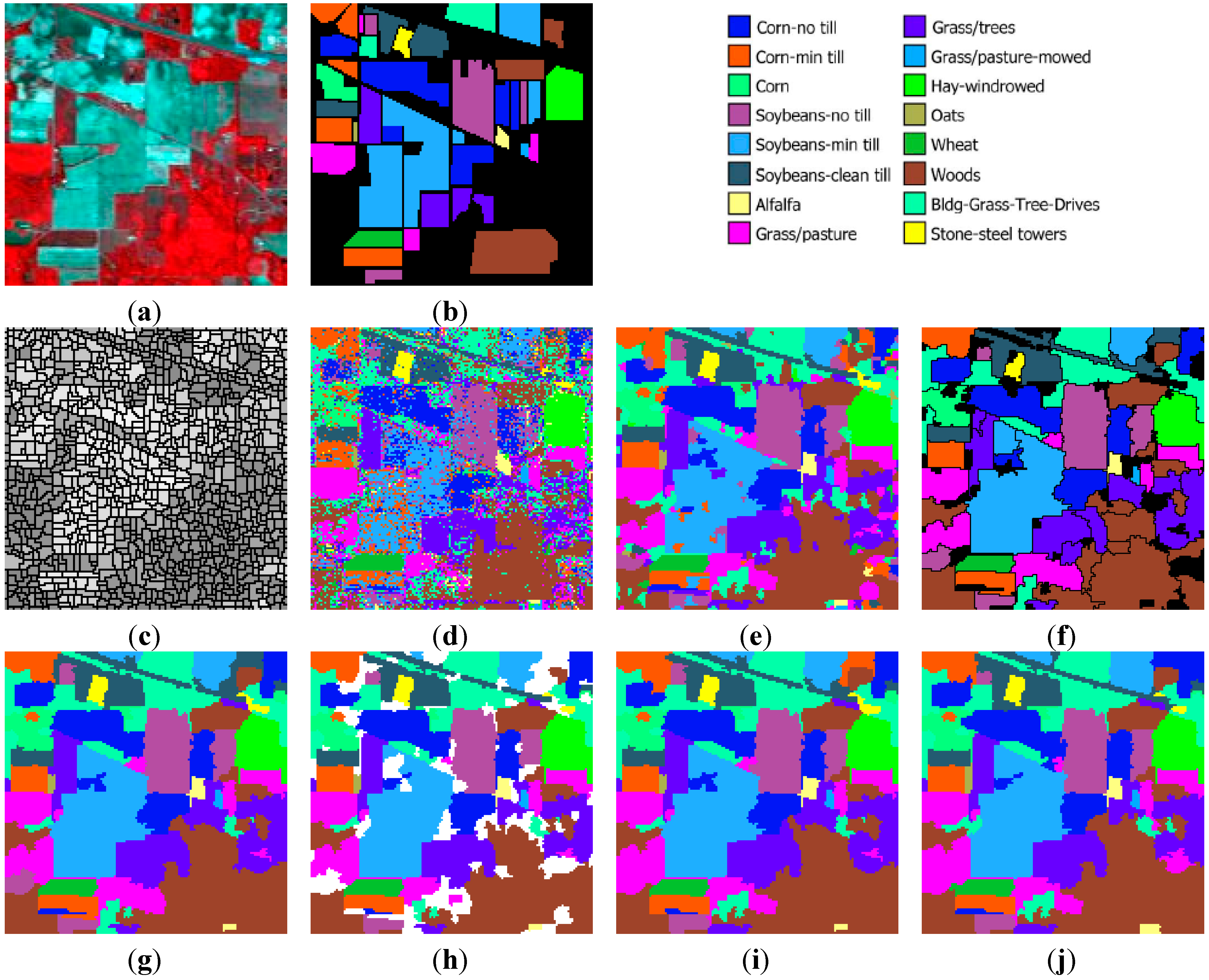
32], and the remaining 200 bands were used in the experiments. A three-band false-color composite and the reference sites are shown in
Figure 8a,b, respectively. The 16 classes of interest existing in this image (mostly different types of crop) are described in
Table 3. The training set is randomly selected from reference data, including 15 samples from the three smaller classes (alfalfa, grass/pasture-mowed, and oats), and 50 samples for the remaining classes. The remaining reference data comprised the test set.
Initially, watershed segmentation is performed as described in
Section 2.1. The resulting map is shown in
Figure 8c, where each watershed is represented by its mean spectral value on an arbitrarily chosen band (Band 120). As expected, the image is highly oversegmented, containing small, well-shaped, and compact watershed regions. This fine segmentation result forms the initial map of structural elements used as the basis for the GeneSIS operation. After the assignment of the watershed pixels to their neighboring objects, a segmentation map with 1109 initial watersheds is created.
Pixel-based classification is next performed by fuzzy output SVM using the entire space of 200 spectral bands. The RBF kernel was considered, while the optimal parameters were chosen by 5-fold cross validation:
and
. After hardening of fuzzy degrees, we obtain the supervised classification map shown in
Figure 8d. As can be seen, the majority of the fields are correctly classified. Nevertheless, there exists a strong confusion between the spectrally similar corn and soybean types, which produces many misclassifications within certain fields of the corresponding classes. Apparently, the absence of contextual information leads to a highly fragmented SVM map.
Next, we compute the membership degrees of watershed objects via decision fusion by fuzzy integral. After CC labeling we obtain map
, shown in
Figure 8e. As can be seen, although the salt and pepper effect is considerably reduced, adequate misclassifications between the spectrally mixed classes still remain. In the marker selection stage, we set
as the size of structures to be marked, in order to enable GeneSIS to recognize the smallest reference field (oats). The global threshold of fuzziness
is set to a low value, specifically
, due to the aforementioned spectral mixings. As a result, 714 watersheds are selected for marking.
In the following, we proceed to image segmentation by GeneSIS. A typical segmentation map obtained by GeneSIS is displayed in
Figure 8f. We can notice that the extracted segments cover mostly the large and homogeneous areas of the image, achieving also a good match with the respective reference fields. It is also remarkable that GeneSIS is now able to cover a whole reference field with a single extraction, without splitting it in more segments. In addition, it should be stressed that the extracted objects appear with varying shapes and irregular boundaries. Particularly, their shapes are delineated from the boundaries of watershed objects included in the BSFs, while the polygonal representation of the chromosome facilitates the extraction of non-convex objects. These are some major differences to the pixel-based version of GeneSIS, where the delineated boundaries and the shape of the objects were strongly constrained by the rectangular shape of the BSF. Finally, an interesting property of the GeneSIS approach is that it is a marker-driven but scale-free segmentation algorithm. Specifically, for each local region, OEA automatically achieves the best compromise between coverage and consistency, according to its size and homogeneity,
i.e., it adapts the segment to be extracted to the existing local scale. Hence, GeneSIS does not necessitate the prior determination of a scale parameter to control the segmentation results, contrary to other segmentation methods.
Figure 8.
Indiana image: (a) three-band false color composite, (b) reference sites, (c) watershed segmentation map, (d) classification map by SVM, (e) initial segmentation via CC labeling, (f) segmentation map after GeneSIS (black areas denote the yet uncovered small regions of the image), (g) final classification map, (h) total agreement map after 30 runs, (i) classification map after FMV-fusion, and (j) classification map after MSF-based fusion.
As a last step, the remaining components are merged to the previously extracted objects via region growing, thus obtaining the final map in
Figure 8g. This map is clearly more homogeneous compared to the initial map of CCs (
Figure 8e), since many of the previous misclassifications have been resolved. This can also be deduced by considering the number of connected components in the two maps. GeneSIS generated on average 70 CCs, considerably fewer than the 217 components appearing in the initial map of
Figure 8e.
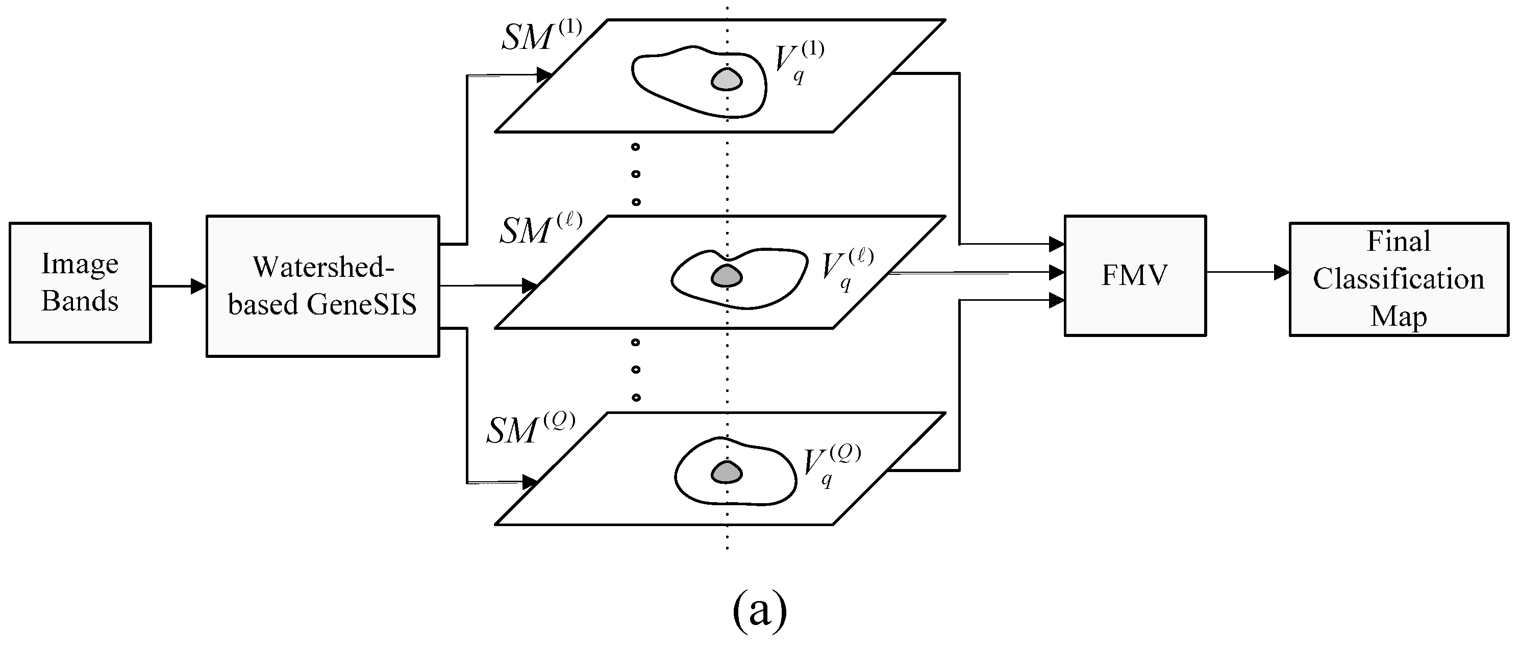
The maps resulting after the fusion of the 30 independent segmentations, using the proposed FMV and the MSF-based fusion methods, are depicted in
Figure 8i,j, respectively. Further,
Figure 8h shows the set of objects (colored areas) that are assigned to the same class by all segmentations, which are used as markers for the MSF-based fusion method. As can be noticed, these objects cover a large portion of the image, comprising mainly the large and homogeneous regions. Hence, the fusion methods operate mostly on the mixed and uncertain parts of the image (white areas in
Figure 8h).
In
Table 2 we compare the two GeneSIS-based approaches,
i.e., the previous pixel-based GeneSIS [
20] and the currently proposed region-based approach, in terms of overall accuracy (OA) and execution time. The new scheme attains better maximum and average overall accuracy, while at the same time indicating enhanced robustness, by reducing the variance of the produced accuracies. However, the main impact of the region-based representation is reflected in the execution time, since the new scheme is 62% faster than the previous one. Particularly, pixel-based GeneSIS requires 15.52 s while the region-based one needs 5.87 s, on average.
Table 2.
Average OA, standard deviation of OA, maximum OA, and execution time for the two GeneSIS versions in Indiana Image.
Table 2.
Average OA, standard deviation of OA, maximum OA, and execution time for the two GeneSIS versions in Indiana Image.
| | Average | Standard Deviation | Max | Time (s) |
|---|
| Pixel-based GeneSIS | 93.61 | 0.39 | 94.51 | 15.2 |
| Region-based GeneSIS | 94.30 | 0.34 | 95.03 | 5.87 |
Table 3 hosts the classification results given by the fusion methods and the competing segmentation algorithms of the literature for the Indiana image. The results are evaluated by means of overall accuracy (OA), average accuracy (AA), kappa coefficient k, and class-specific accuracies. In regard to the above results, the following comments are in order. (1) First, the pixel-wise SVM classification offers by far the worst accuracy compared to the other segmentation-based classification approaches. This finding justifies the need to formulate meaningful objects to be classified, instead of handling single pixels. (2) Both pixel-based and especially the new region-based GeneSIS outperform the accuracy of the initial segmentation map
by 2%–3%. This improvement implies that GeneSIS further homogenizes the input map
by creating a smaller number of segments. On the other hand, it correctly assigns the ambiguous areas of the image, which leads to higher classification accuracies. (3) Both fusion methods achieve better results than an average GeneSIS run, since their OAs are higher than the average OA obtained from the ensemble of segmentations. Especially, the MSF-based fusion method performs slightly higher than the best accuracy attained from the ensemble of 30 segmentations by GeneSIS. This indicates that, through fusion, a significant number of the disagreements existing between the different segmentations is effectively resolved. (4) The spatial PR considerably improves the accuracy of the pixel-based SVM classification. However, both region-based GeneSIS and the two fusion schemes significantly outperform the filtered SVM results by over 5%. This is due to the fact that filtering refines the image components locally, while GeneSIS evaluates much larger areas to formulate the optimal segments. (5) Compared to the other segmentation algorithms, we observe that GeneSIS achieves higher classification performance even in terms of average OA. Moreover, using the MSF-based fusion, GeneSIS offers the highest AA, which shows its ability to sufficiently handle all the classes without underestimating any of them.
Table 3.
Classification accuracies for the Indiana Image.
Table 3.
Classification accuracies for the Indiana Image.
| | SVM | FMV-Fusion | MSF-Fusion | SVM + PR | Initial Map
C | CaHO | HSwC | M-HSEG°p | MSF |
|---|
| DC | SAM | SAM | SAM | SAM | L1 |
|---|
| OA | 76.22 | 94.51 | 95.08 | 89.99 | 91.71 | 93.48 | 92.56 | 93.18 | 93.27 |
| AA | 84.03 | 94.20 | 96.52 | 93.81 | 92.96 | 96.05 | 95.71 | 89.24 | 89.20 |
| k | 73.09 | 93.73 | 94.36 | 88.59 | 90.54 | 92.55 | 91.49 | 92.17 | 92.28 |
| Alfalfa | 87.18 | 92.31 | 92.31 | 100 | 92.31 | 89.74 | 89.74 | 89.74 | 89.74 |
| Corn-notill | 72.62 | 95.09 | 96.17 | 88.95 | 93.28 | 93.21 | 88.95 | 93.64 | 92.85 |
| Corn-min | 67.35 | 88.14 | 83.93 | 80.23 | 81.76 | 85.08 | 85.59 | 88.90 | 90.18 |
| Corn | 76.09 | 97.28 | 97.83 | 98.91 | 97.28 | 100 | 100 | 100 | 100 |
| Grass/Pasture | 92.39 | 96.20 | 96.20 | 95.30 | 96.20 | 96.42 | 96.20 | 96.20 | 94.18 |
| Grass/Trees | 95.41 | 99 | 97.99 | 99.43 | 98.71 | 99 | 99.14 | 96.84 | 100 |
| Grass/pasture-mowed | 100 | 100 | 100 | 100 | 100 | 100 | 100 | 100 | 100 |
| Hay-windrowed | 97.04 | 99.77 | 99.77 | 98.86 | 99.77 | 99.77 | 99.77 | 99.77 | 99.77 |
| Oats | 80 | 60 | 100 | 80 | 60 | 100 | 100 | 0 | 0 |
| Soybeans-notill | 77.12 | 99.24 | 95.10 | 93.03 | 96.41 | 98.80 | 99.02 | 82.03 | 82.24 |
| Soybeans-min | 58.35 | 88.30 | 93.05 | 80.73 | 82.13 | 90.28 | 88.75 | 94.38 | 94.25 |
| Soybean-clean | 84.40 | 97.16 | 97.16 | 95.39 | 96.81 | 95.21 | 95.74 | 96.28 | 96.45 |
| Wheat | 99.38 | 99.38 | 99.38 | 99.38 | 99.38 | 100 | 99.38 | 99.38 | 100 |
| Woods | 88.91 | 97.91 | 97.91 | 95.66 | 96.78 | 90.84 | 90.84 | 91 | 91 |
| Bldg-Grass-Tree-Drives | 72.73 | 99.70 | 99.70 | 95.15 | 98.79 | 98.48 | 98.18 | 99.70 | 98.79 |
| Stone-steel towers | 95.56 | 97.78 | 97.78 | 100 | 97.78 | 100 | 100 | 100 | 97.78 |
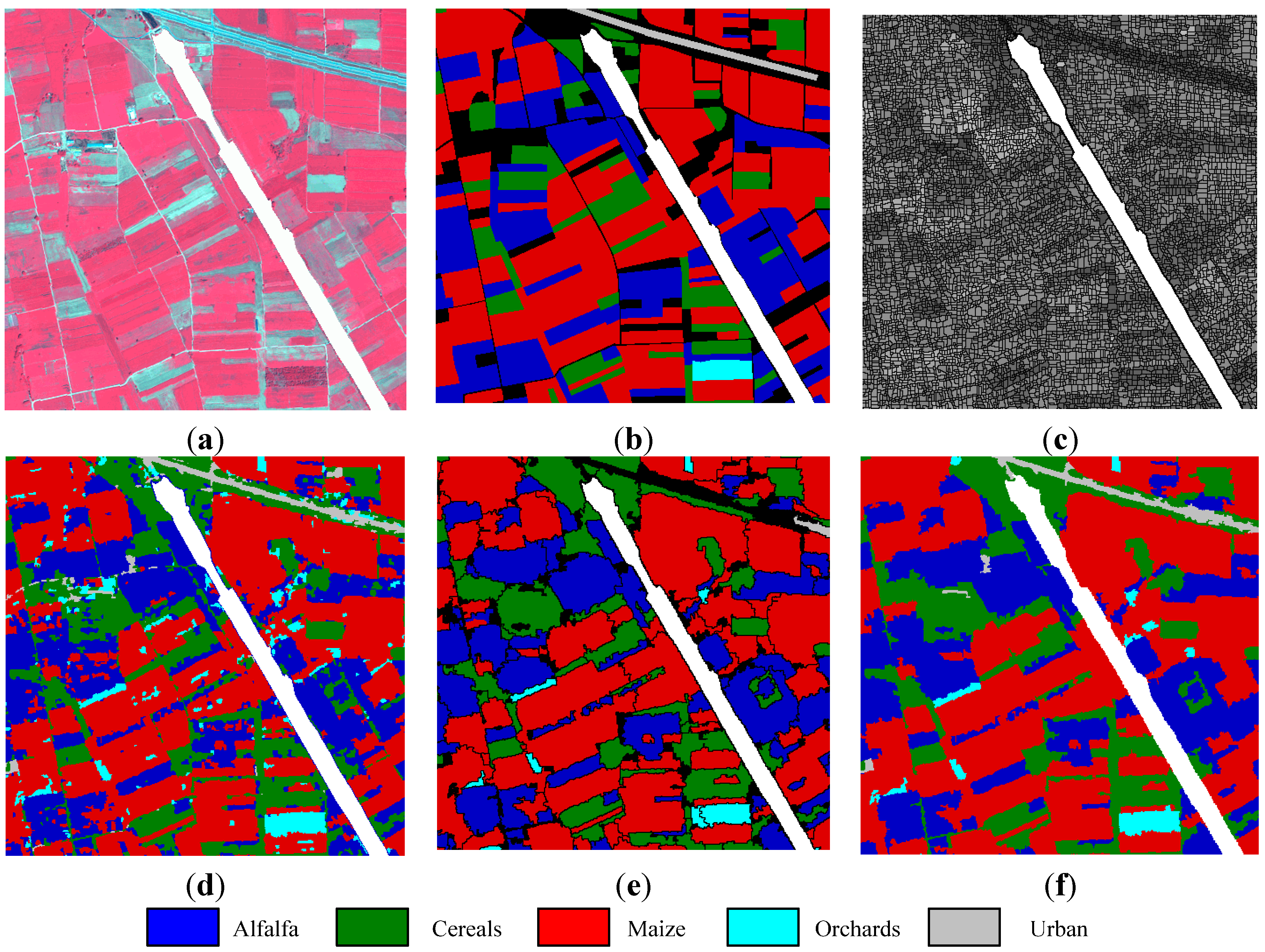
5.2. Koronia Image
Koronia image is an IKONOS bundle image acquired over a cultivated area around Lake Koronia, northern Greece. The image has four spectral channels (three visible and one near-infrared) with a spatial resolution of 4 m/pixel. Our experiments were conducted on a sub-image of
pixels, extracted from the agricultural zone nearby the lake. Five classes of interest were identified: alfalfa, cereals, maize, orchards, and urban areas, with the first three being the major ones. The reference sites are collected after extensive field survey and photo-interpretation by the experts, in combination with high-resolution orthophotos. The training set was selected randomly from the reference data and comprises 300 samples for the first three classes and 150 for the remaining two. The rest of the reference data comprised the test set, as detailed in
Table 5.
Pixel-wise SVM classification in this image is performed using an advanced space of 53 features overall, including the original four bands of the image, transformed spectral features (TSF), and textural features. Particularly, we consider the intensity (I) and hue (H) from the HIS color space, and the three data structures from Tasseled Cap transformation, suitable for vegetation representation. Furthermore, we examine 16 features from Gray-Level Co-occurrence Matrix (GLCM) and 28 wavelet features. Textural features are computed from fixed local windows around pixels of appropriate size. A detailed discussion on the derivation of the above features can be found in [
33].
Figure 9.
Koronia image: (a) three-band false color composite, (b) reference sites, (c) watershed segmentation map, (d) initial segmentation map after CC labeling, (e) segmentation map after GeneSIS (black areas denote the yet uncovered regions of the image), and (f) classification map after FMV-fusion.
For clarity in presentation, the obtained results will be depicted on a portion of
pixels of the whole study area. The three-band false color image and the reference data of this portion are shown in
Figure 9a,b, respectively. The initially oversegmented map is shown in
Figure 9c, where the watershed objects are depicted on Band 4. After the assignment of watershed pixels to their neighboring objects, the set of the initial structural elements comprises 43,565 watersheds. For the pixel-wise SVM classification, the optimal parameters
C and
γ were chosen through five-fold cross validation:
and
. After derivation of the watershed fuzzy degrees, we obtain the map shown in
Figure 9d. The visual assessment of the map shows that the majority of fields are correctly classified. However, within some large physical structures,
i.e., crop fields, there exist small patches being classified erroneously. For instance, some components within certain maize fields are wrongly assigned to the alfalfa class. By observing the size of the fields existing in the study area, the marking threshold is set to
. In this case, the global threshold of fuzziness
is set to a higher value compared to the Indiana image, specifically
, since the classification results are more precise here. As a result, 21,945 watersheds are selected for marking.
A typical segmentation after GeneSIS is shown in
Figure 9e. The extracted objects follow the size and orientation of ground truth structures, especially avoiding oversegmentation of large ground components. GeneSIS generated on average 475.5 CCs, considerably smaller than the 4178 connected components existing in the initial map
, shown in
Figure 9d. Finally, the obtained map after FMV-fusion is depicted in
Figure 9f.
In
Table 4, we present the comparative results of the two GeneSIS variants. Similar conclusions to the Indiana image can also be drawn for this case study. For the region-based GeneSIS, we notice a small increase in average and maximum OA, while the standard deviation of the results is slightly decreased. As in the previous image, the critical asset of the region-based representation lies in the substantial reduction of the average execution time, in this case by a percentage of 57%.
Table 5 summarizes the results from GeneSIS after fusion and the comparative methods. It can be seen that the proposed segmentation fusion methods exhibit similar or higher OA than the best one in the ensemble of segmentations. Both fusion methods outperform the competing methods in terms of OA and AA in the majority of the different classes. Finally, the three GeneSIS-based methods improve the results of the initial segmentation map
and the filtered SVM+PR results by a percentage of 2%.
Table 4.
Average OA, standard deviation of OA, maximum OA, and execution time for the two GeneSIS versions in Koronia Image.
Table 4.
Average OA, standard deviation of OA, maximum OA, and execution time for the two GeneSIS versions in Koronia Image.
| | Average | Standard Deviation | Max | Time (m) |
|---|
| Pixel-based GeneSIS | 82.93 | 0.19 | 83.26 | 17.07 |
| Region-based GeneSIS | 83.53 | 0.12 | 83.74 | 7.40 |
Table 5.
Classification accuracies for the Koronia image.
Table 5.
Classification accuracies for the Koronia image.
| - | SVM | FMV-Fusion | MSF-Fusion | SVM + PR | Initial Map
C | CaHO | HSwC | M-HSEG°p | MSF |
|---|
| DC | L1 | SAM | SAM | SAM | L1 |
|---|
| OA | 77.37 | 83.87 | 83.59 | 81.48 | 81.28 | 82.30 | 82.49 | 80.52 | 81.44 |
| AA | 78.94 | 85.84 | 85.93 | 83.75 | 83.05 | 82.71 | 81.57 | 84.00 | 78.54 |
| k | 64.19 | 73.71 | 73.21 | 70.29 | 69.83 | 71.31 | 71.36 | 68.43 | 69.78 |
| Alfalfa | 64.78 | 70.01 | 69.40 | 69.49 | 67.18 | 68.58 | 66.09 | 63.95 | 66.47 |
| Cereals | 81.17 | 85.43 | 85.12 | 83.77 | 83.78 | 85.07 | 85.88 | 84.78 | 83.40 |
| Maize | 81.94 | 89.82 | 89.69 | 86.25 | 87.09 | 88.00 | 89.38 | 86.76 | 87.96 |
| Orchards | 80.61 | 93.40 | 94.42 | 88.24 | 92.14 | 93.40 | 91.82 | 92.93 | 65.09 |
| Urban | 86.19 | 90.53 | 91 | 90.99 | 85.03 | 78.47 | 74.69 | 91.58 | 89.80 |
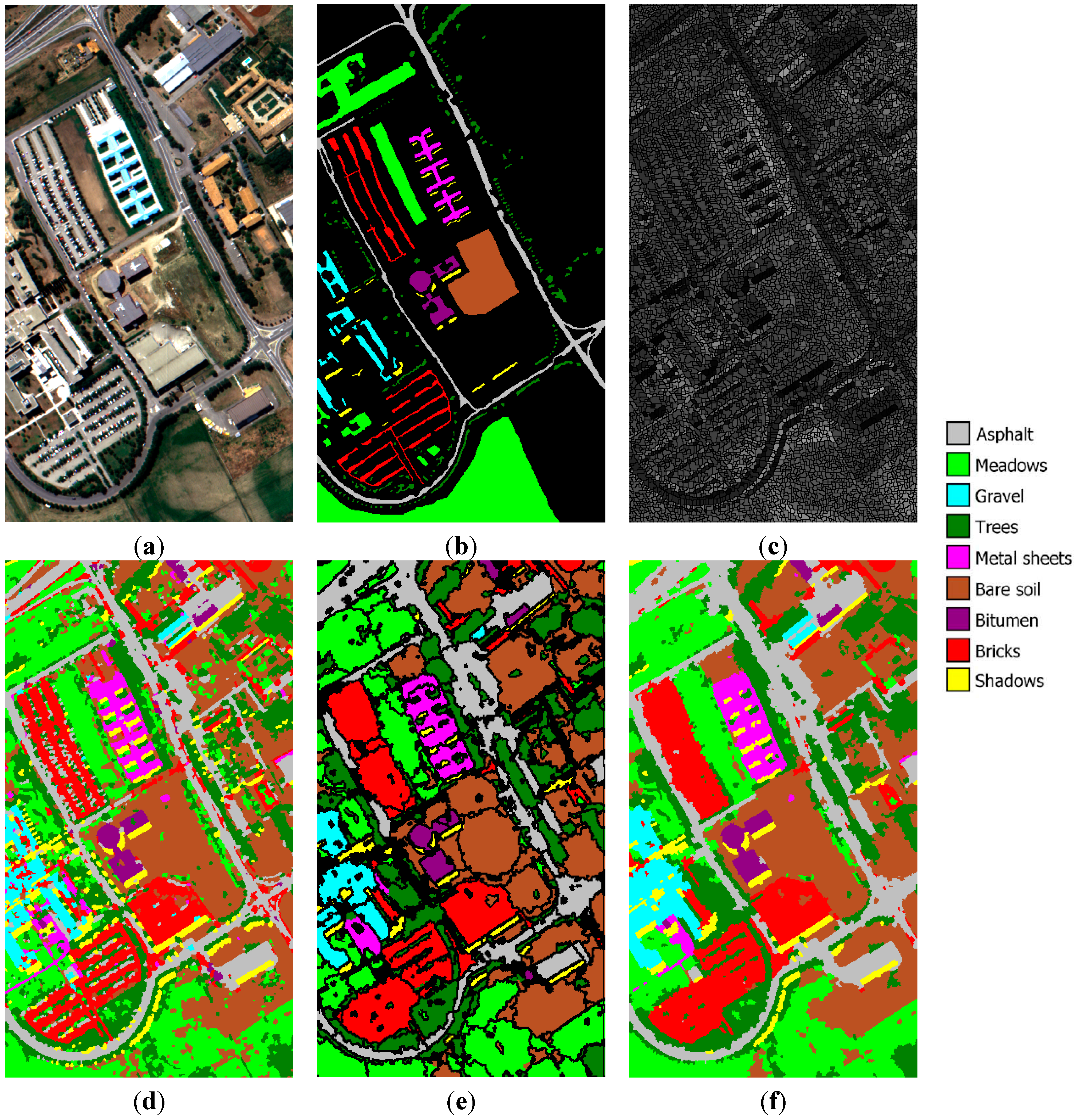
5.3. University of Pavia Image
The University of Pavia image is a hyperspectral image acquired by the ROSIS-03 sensor over the University of Pavia, northern Italy. The spatial dimension of the image is
and its spatial resolution is 1.3 m/pixel. The full spectral range of the initially recorded image contains 115 bands (ranging from 0.43 to 0.86 μm). The 12 most noisy channels were removed and the remaining 103 spectral bands were used in our experiments. The comparison of the two GeneSIS approaches are shown in
Table 6. The nine classes of interest existing in the terrain are detailed in
Table 7. For the exact number of training and test samples per class, the reader can refer to [
20]. A three band true color composite and the reference sites are shown in
Figure 10a,b, respectively.
Figure 10.
University of Pavia image: (a) three-band false color composite, (b) reference sites, (c) watershed segmentation map, (d) initial segmentation map after CC labeling, (e) segmentation map after GeneSIS, and (f) classification map after FMV-fusion.
Figure 10.
University of Pavia image: (a) three-band false color composite, (b) reference sites, (c) watershed segmentation map, (d) initial segmentation map after CC labeling, (e) segmentation map after GeneSIS, and (f) classification map after FMV-fusion.
Table 6.
Average OA, standard deviation of OA, maximum OA, and execution time for the two GeneSIS versions in University of Pavia Image.
Table 6.
Average OA, standard deviation of OA, maximum OA, and execution time for the two GeneSIS versions in University of Pavia Image.
| | Average | Standard Deviation | Max | Time (m) |
|---|
| Pixel-based GeneSIS | 88.41 | 0.22 | 88.96 | 3.92 |
| Region-based GeneSIS | 89.86 | 0.65 | 90.95 | 1.07 |
Table 7.
Classification accuracies for the University of Pavia image.
Table 7.
Classification accuracies for the University of Pavia image.
| | SVM | FMV-Fusion | MSF-Fusion | SVM + PR | Initial Map
C | CaHO | HSwC | M-HSEG°p | MSF |
|---|
| DC | SAM | SAM | SAM | SAM | SAM |
|---|
| OA | 81 | 90.49 | 89.56 | 87.19 | 86.55 | 88.45 | 87.51 | 89.96 | 88.48 |
| AA | 88.15 | 94.95 | 95.01 | 92.73 | 93.41 | 94.45 | 93.21 | 95.39 | 93.30 |
| k | 75.74 | 87.59 | 86.43 | 83.46 | 82.70 | 85.07 | 83.87 | 86.97 | 85.11 |
| Asphalt | 76.51 | 94.91 | 93.78 | 89.58 | 90.40 | 93.51 | 90.75 | 97.73 | 97.26 |
| Meadows | 73.59 | 83.42 | 81.53 | 79.03 | 76.91 | 79.22 | 78.81 | 80.80 | 78.76 |
| Gravel | 71.35 | 85.51 | 89.20 | 75.37 | 81.10 | 86.39 | 85.40 | 92.29 | 89.48 |
| Trees | 98.70 | 96.46 | 96.09 | 99.52 | 98.21 | 98.73 | 98.52 | 96.91 | 95.54 |
| Metal sheets | 99.01 | 99.91 | 99.91 | 100 | 99.46 | 99.82 | 99.82 | 99.91 | 99.91 |
| Bare soil | 91.80 | 98.88 | 98.47 | 98.08 | 97.22 | 98.21 | 97.05 | 97.88 | 97.73 |
| Bitumen | 91.54 | 99.59 | 100 | 94.90 | 98.78 | 97.35 | 98.17 | 98.88 | 99.18 |
| Bricks | 91.14 | 99.26 | 99.11 | 98.19 | 98.72 | 99.20 | 98.81 | 99.79 | 99.85 |
| Shadows | 99.75 | 96.60 | 96.98 | 99.87 | 99.87 | 97.61 | 91.57 | 94.34 | 82.01 |
The initially obtained watershed segmentation map is depicted upon Band 80 in
Figure 10c. After the assignment of watershed pixels to their neighboring objects, the set of the initial structural elements comprises 9152 watersheds. The optimal parameters
C and
γ of the pixel-based SVM classification were chosen through five-fold cross validation:
and
. The obtained SVM map is next combined with the watershed segmentation via the fuzzy integral approach, and the initial map
is obtained, as shown in
Figure 10d. As can be seen, most of the class areas are correctly classified, except mainly from the large meadows region in the lower part of the image, which is confused with the trees and bare soil. This can be interpreted by observing
Figure 10a, where it can easily be seen that this region is spectrally heterogeneous although it belongs to the same class. In order for GeneSIS to be able to recognize some small components of trees and shadows, the marking threshold parameter was set here to
. The global threshold of fuzziness
is set to a medium value
, since the classification results are of moderate precision compared to the previous two paradigms. As a result, 4735 watersheds are selected for marking. Finally, in
Figure 10e,f, we can see a typical segmentation after GeneSIS and the final map obtained after FMV fusion, respectively. Although most of the extracted segments follow the orientation and shape of the ground truth objects, there are still some misclassifications at the lower part of the image. This can be attributed to the erroneous marking of some initial objects, which were initially misclassified by the SVM.
The comparison of the two GeneSIS approaches, through
Table 6, leads to conclusions similar to those in the previous case studies. The region-based GeneSIS exhibits higher average and maximum accuracies of about 1.5%–2%, although the standard deviation of the results is increased. The most obvious effect of the region-based representation lies again in the execution time, which is on average decreased by a percentage of 73%.
Table 7 summarizes the results from GeneSIS after fusion and the comparative methods. It can be seen that the GeneSIS-based methods clearly outperform both the initial segmentation map
and the SVM+PR results. Noticeably, this latter method achieves high AAs for the small classes, while on the other hand it is unable to correctly classify the larger ones. Finally, the FMV-fusion method performs better than the competing methods in terms of OA and
k, with the exception of M-HSEG
op, which is superior in terms of AA.


 ,
, 


