Article

Index of Soil Moisture Using Raw Landsat Image Digital Count Data in Texas High Plains

1
Department of Plant and Soil Science, Texas Tech University, Lubbock, TX 79409, USA
2
Department of Plant and Soil Science, Texas Tech University and Research Center, Texas A&M, Lubbock, TX 79409, USA
*
Author to whom correspondence should be addressed.
Remote Sens. 2015, 7(3), 2352-2372; https://doi.org/10.3390/rs70302352
Submission received: 12 September 2014 / Revised: 15 January 2015 / Accepted: 29 January 2015 / Published: 26 February 2015

Abstract

:
The growth and yield of crops in the arid and semi-arid regions of the world is driven by the amount of soil moisture available to the crop through rainfall and irrigation. Various methods have been developed for quantifying the soil moisture status of agricultural crops. Recent technological advances in remote sensing have shown that soil moisture can be measured with a variety of remote sensing techniques, each with its own strengths and weaknesses. In this study, building on of the strengths of multispectral satellite imagery, a new approach is suggested for estimating soil moisture content. A soil moisture index, the Perpendicular Soil Moisture Index (PSMI), is proposed; it is evaluated using raw image digital count (DC) data in the red, near-infrared, and thermal infrared spectral bands. To test this approach, soil moisture was measured in 18 agricultural fields in the semi-arid Texas High Plains over two years and compared to corresponding PSMI values determined from Landsat image data. These results showed that PSMI was strongly correlated (R2 = 0.79) with observed soil moisture. It was further demonstrated that maps of PSMI developed from Landsat imagery could be constructed to show the relative spatial distribution of soil moisture across a region. While further study is needed to determine the exact relationship between PSMI and soil moisture in larger areas with different climates, this study suggests that PSMI is a good indicator of soil moisture and has potential for operationally monitoring soil moisture conditions at the field to regional scales.

1. Introduction

In the arid and semi-arid regions of the world, the growth and yield of agricultural crops is inexorably linked to the amount of water available from precipitation and/or irrigation. Many studies [1,2,3,4,5] have shown a linear relationship between crop dry mass or yield and soil moisture over the growing season. The ability to quantify soil moisture content allows researchers to study the interaction of crops and their environment and supports practical crop production activities such as irrigation scheduling. Accurate assessment of this variable is difficult because typical field methods are complex and expensive and local scale variations in soil properties, terrain, and vegetation cover make selection of representative field sites difficult if not impossible [6,7,8].
Remotely sensed observations of reflected and emitted electromagnetic (EM) radiation appear to be at least a partial solution to the spatial sampling problem. Satellite imagery provides the capability to produce spatially comprehensive measurements of surface environmental conditions. In contrast with field measurement, remote sensing techniques are promising because they are explicitly spatial measurements that can be acquired at relatively low cost [9,10]. If variations in measured EM emittance can be related to surface moisture conditions, then both regional variations and local spatial heterogeneity of soil moisture conditions may be determined [11,12].
Over the last quarter century, much research has been done on the use of remote sensing observations to evaluate soil moisture conditions. Studies which employ measurements from solar reflectance [13,14], thermal infrared wavelengths [7,13,15,16,17,18,19,20], and microwaves [13,21,22,23,24,25] have all shown potential in this area.
The basic idea of using satellite imagery to estimate soil moisture is that soil moisture affects surface characteristics that can be observed through remote sensing. These include bio-physical factors such as vegetation cover, observed through vegetation indices (VI), and the surface energy balance, observed through surface temperature (Ts). Ts is a good indicator of the energy balance on both regional and global scales [26,27,28]. Ts has been recognized as one of the biophysical factors sensitive to soil moisture content for quite a while [12,29]. Stomata of stressed plants close to minimize water loss by transpiration, which results in a decreased latent heat flux [30]. To balance the energy flux, there is a concurrent increase in sensible heat flux associated with warmer leaf temperatures and increased Ts [30]. In general, VI decreases and Ts increases with decreasing soil moisture. The combination of Ts and VI may provide useful information for quantitative detection of the spatial and temporal distribution of soil moisture. Goward and Hope [31] and Price [20] plotted VI vs. Ts to form a Ts-VI feature space. This feature space often exhibited a triangular shape [20,32] or a trapezoid shape [12] if a full range of fractional vegetation cover and soil moisture is represented in the data. Basically, a triangle emerges because the range of surface radiant temperature decreases as the vegetation cover increases [16,33].
During the 1990s, this “triangle method” was used in mapping soil moisture content based on Ts-VI feature space without the need for ancillary atmospheric and surface data. Since then, the Ts-VI feature space has been widely used in land surface classification, soil moisture content monitoring, and surface energy fluxes [28,34,35,36,37,38,39,40,41,42,43,44]. Moran et al. [12] reported that the Ts-VI space could be represented by a “trapezoid” shape which they called the Vegetation Index/Temperature Trapezoid (VITT). Based on this, they developed the Water Deficit Index (WDI), which accounts for partially vegetated surfaces. Jiang and Islam [45,46] suggested a technique for the estimation of regional latent heat flux (LE), based on the combination of the Ts-NDVI scatterplot and a simplified form of the Priestley-Taylor equation for LE fluxes, where some parameters of the latter were derived from the Ts-NDVI pixel envelope. Sandholt et al. [47] improved the triangle method by linking the plot of Ts-VI with an index, which they termed the Temperature-Vegetation-Dryness-Index (TVDI). The main assumption was that soil moisture content is the main source of variation for Ts and that TVDI is related to surface soil moisture due to changes in thermal inertia and evaporative control of the available energy (i.e., net radiation (Rn), soil heat flux (G)). Stisen et al. [35], using data from METEOSAT SEVIRI and ground observation from a test site in South Senegal, West Africa, proposed that the use of the (Ts–Tair) measure in the Jiang and Islam [48] approach be substituted by either Ts recorded at 12:00 local time or by the surface temperature difference (dTs) calculated between 12:00 and 8:00 local time. Mallick et al. [49] summarize the most important sources of uncertainty in soil moisture estimation—which to some degree also apply to the surface energy fluxes estimation—from the Ts-VI domain. Recently Zhang et al. [34] proposed the Temperature Rising Rate Vegetation Dryness Index (TRRVDI) based on a triangle constructed using the mid-morning land surface temperature (Ts) rising rate and the VI to estimate the regional soil water content. The temperature at the dry edge of the triangle is determined by the surface energy balance principle. The temperature at the wet edge is assumed to be equal to the air temperature.
While the Normalized Difference Vegetation Index (NDVI) has been found to be an effective indicator of vegetation conditions [47,50], it is a rather conservative indicator of soil moisture status because there is a time lag between the occurrence of a change in soil moisture and the observed change in NDVI. Thus, NDVI-based methods may not be effective in rapid monitoring of soil moisture conditions.
All of the previously discussed methods require converting thermal remote sensing data to surface temperature, which involves precise calibration of the satellite surface temperatures and initialization of the land surface model with atmospheric measurements. This conversion and calibration is time-consuming and collection of additional information can be expensive. In addition, small errors in computed surface temperature might yield unreasonable values of the surface energy fluxes [16,33]. Since satellite-derived temperatures are subject to an accuracy of ±1–2 °C, the estimates derived from the satellite measurements may be subject to considerable uncertainty without an independent and easily accessible means of verifying or constraining the input [16]. Another drawback of these methods involves the interpretation of the Ts-VI feature space. There is difficulty in establishing the “dry edge” of the feature space, and many methods have been proposed for its calculation [28,34,36,51]. Most studies have not found the location of an image pixel value relative to this edge to be practical for soil moisture monitoring. Since the location of a pixel in the Ts-VI space is influenced by many factors, including the type of surface, the slope of this edge is not unique for different atmospheric and surface moisture conditions [47].
A simple and robust remote sensing-based method for estimating soil moisture that is applicable to different vegetation conditions would be of great interest to those interested in monitoring soil moisture. In particular, a method that utilizes raw remote sensing data in the visible, near-infrared and thermal infrared without calibration or conversion to surface reflectance or temperature would greatly enhance its application. In this study, we describe the development of an index—the Perpendicular Soil Moisture Index (PSMI)—that has these characteristics. Using field data and Landsat image data, we show the relationship between this index and soil moisture. Specific objectives of this study include (1) to investigate the potential of using a combination of visible, near-infrared and thermal infrared to estimate soil moisture from space and to find an algorithm that is suited for monitoring soil moisture; (2) to compare the resulting index (PSMI) with soil moisture from direct measurements; and (3) to demonstrate how this index can be used with readily available Landsat data to map the spatial distribution of soil moisture conditions on a regional scale and monitor its change over time.

2. Methods and Materials

2.1. Theory

When the values of vegetation ground cover (GC) are plotted vs. corresponding values of surface temperature (Ts) for pixels comprising a medium-resolution multispectral satellite image of an agricultural region, a characteristic distribution of points is produced. An example is shown in Figure 1A. Figure 1B presents a diagrammatic representation of this distribution—this is the classic “trapezoid” interpretation of the VI-Ts feature space described in the previous section. The distribution of points in the figure results from the moisture status of vegetation and soil in the scene and the relative amounts of vegetation and soil that are present within the pixels that make up the scene.
Figure 1. Ground cover (GC) plotted vs. surface temperature (Ts). (A) Actual distribution of GC vs. Ts for pixels in a Landsat-7 image of an agricultural region; (B) Diagrammatic representation of features of the distribution of Ts-GC space. Points ad indicate the vertices of the trapezoidal representation of the distribution of points.
Remotesensing 07 02352 g001
The lower left part of this distribution is represented by low vegetation cover pixels with low surface temperature and high soil moisture content (point a) and the lower right zone is represented by pixels having low moisture content/minimum evapotranspiration with low vegetation cover and high temperature (point b). Also, the upper left zone represents densely vegetated covered pixels with high soil moisture/maximum transpiration and low temperature (point c) and the upper right zone is densely vegetated covered pixels with low moisture content/minimum transpiration and high temperature (point d).The line connecting point a to point c is called the wet edge, and the line connecting point b to point d is called the dry edge. Thus, the distribution of points in Figure 1 should be associated with an underlying gradient in soil moisture progressing from relatively moist conditions along the wet edge to relatively dry conditions along the dry edge.
One of the goals of this study was to develop an index of soil moisture from raw remote sensing image digital count (DC) data in the visible, near-infrared and thermal infrared spectral bands, like those available from Landsat. For the distribution of pixel values in Figure 1, GC can be directly estimated from image DC values in the red and near-infrared spectral bands using the procedure described by Maas and Rajan [52,53]. Unfortunately, Ts cannot be estimated in a similar manner directly from raw DC data in the thermal infrared spectral band, and its determination often requires additional information on surface emissivity and atmospheric conditions. However, image DC values in the thermal infrared spectral band (TIR) should be proportional to Ts. Figure 2 shows a distribution that is similar to Figure 1A, but in this case GC has been plotted vs. TIR that is used in calculating Ts, although the absolute relationship between TIR and Ts might vary between image acquisitions due to changes in surface emissivity and atmospheric conditions over time. This proportionality could allow TIR to be used as a surrogate for Ts in developing an index of soil moisture if acquisition-to-acquisition variations in TIR could be removed or minimized. A procedure aimed at achieving this is described in the next section.

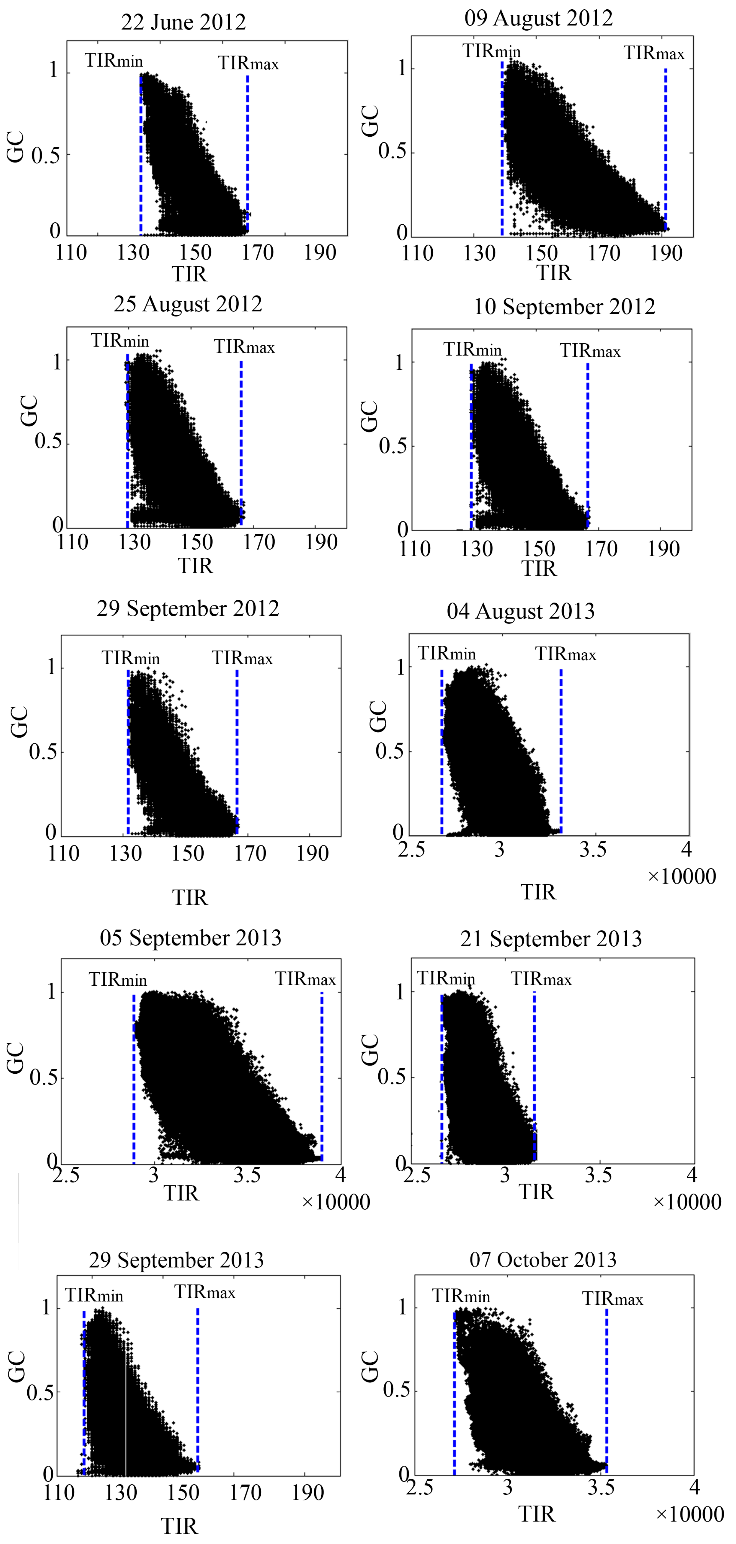
2.1.1. Normalizing TIR-GC Space

Atmospheric conditions and their effects on TIR data are different from day to day, so images that are acquired on different dates often have different ranges in TIR values. TIR-GC spaces that are built for different acquisition dates may be different in terms of absolute values and may be difficult to compare. One way to remove or reduce the absolute differences would be to normalize the values to a range of 0 to 1. TIR could be normalized by the maximum and minimum values of TIR in the image data. As shown in Figure 1, the maximum and minimum values of Ts (Ts,max and Ts,min, respectively) can usually be identified for images of agricultural regions [16,54,55]. Ts,min usually corresponds to non-stressed full canopy (point c), while Ts,max usually corresponds to dry bare soil (point b). For a given image acquisition, the distribution of points in Ts-GC space will be qualitatively similar to the distribution of points in TIR-GC space, so there will be a maximum value of TIR (TIRmax) that corresponds to Ts,max and a minimum value of TIR (TIRmin) that corresponds to Ts,min (Figure 2). Thus, TIR values for an image can be normalized using the following relationship,
TIRi,norm = (TIRi − TIRmin)/(TIRmax − TIRmin)
where TIRi is the TIR value for a given image pixel and TIRi,norm is its normalized value. Normalizing TIR using this procedure puts TIR values within the range from 0 to 1, thereby minimizing acquisition-to-acquisition variations related to surface emissivity and atmospheric conditions. It also conveniently puts both axes of the TIR-GC space into the same range (0 to 1).
One possible limitation to this approach is that the distribution of points in the TIR-GC space for an image must allow identification of points corresponding to the TIRmin and TIRmax used in normalizing TIRi. It has been our experience that, for agricultural regions with a mixture of field crops, perennial pastures, and natural vegetation, the distribution of image pixel values will usually allow identification of these two vertices during most of the growing season. However, the authors recognize that the approach in the form described in this article might not be directly applicable to all situations.
Figure 2. Result of plotting GC vs. raw thermal infrared digital count data (TIR) for pixels making up a medium-resolution multispectral satellite image of an agricultural region.
Remotesensing 07 02352 g002

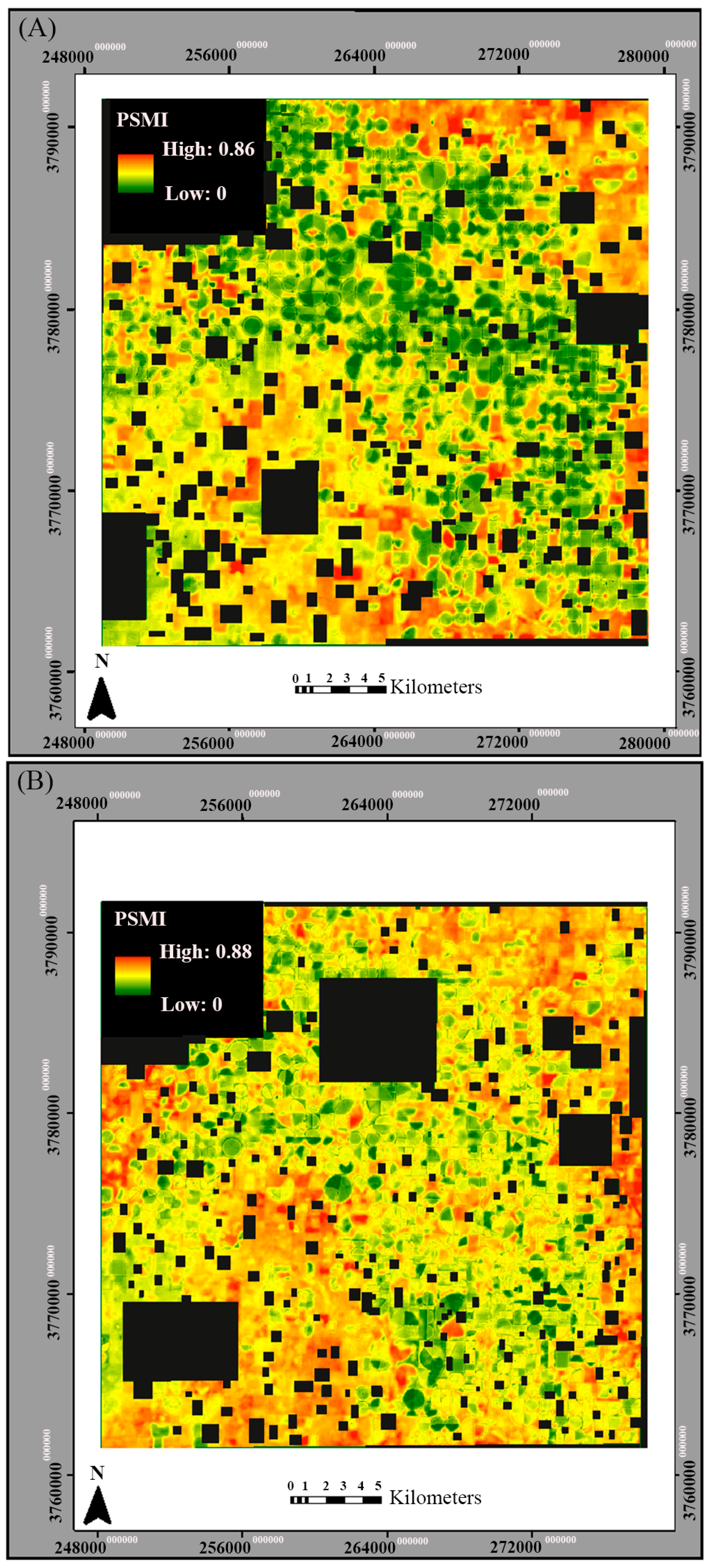
2.1.2. Perpendicular Soil Moisture Index

As stated previously, there is a gradient in soil moisture progressing from relatively moist conditions along the wet edge to relatively dry conditions along the dry edge in Figure 1B. The exact direction of this gradient relative to the TIRnorm and GC axes is unknown. However, the dry edge of the distribution likely represents the driest soil moisture conditions over the imaged scene, which suggests that the gradient in soil moisture should be roughly perpendicular to the orientation of the dry edge.
Figure 3 shows a method based on this assumption for calculating a quantity that should be proportional to soil moisture. To calculate this quantity, a straight line with a slope of −1 (line “B” in Figure 3) is placed through the theoretical point with GC = GCmin = 0 and TIRnorm = TIR norm,min = 0 in the TIRnorm-GC space (point e in Figure 3). This line will bisect the coordination system. The choice of a slope of −1 is somewhat arbitrary but should place the orientation of the line roughly perpendicular to the soil moisture gradient. This line is used as a baseline for measuring distance along the gradient. Considering the theoretical “wet edge” instead of observed sloping wet edge may lead to an error at low GC values.
The perpendicular distance measured from the baseline “B” to any point in the TIRnorm-GC space should be proportional to soil moisture conditions at that point. For the bare soil, the distance from any points in the TIRnorm-GC reflectance space to the line “B” represents the drought severity of the non-vegetated surface. For a vegetated surface, the distance from line “B” to any points in the TIRnorm-GC spectral space may indicate the drought severity of a mixed pixel. That is, the farther the distance, the less the soil moisture or vice versa. An example is shown in Figure 3, where the line between point e and point f represents this distance. This distance Di can be calculated as follows,
D i = ( TIR i , norm + GC i ) / 2
where TIRi,norm and GCi are the normalized TIR and GC values, respectively, for a point in the TIRnorm-GC space. As Di increases, soil moisture decreases. Mathematically, Equation (2) is similar to the Perpendicular Vegetation Index [56].
Figure 3. Diagrammatic representation of the perpendicular distance from a point (f) in the TIRnorm-GC space to the baseline “B” passing though the origin (point e).
Remotesensing 07 02352 g003
While the determination of Di is intended to account for the main variation in soil water content along the gradient between the wet edge and dry edge, a secondary effect on soil moisture can be observed that can be related to the variation in GC across the TIRnorm-GC space. An example is shown in Figure 4. Point g in the Figure 4 represents a bare soil pixel (GC = 0), while point h corresponds to a pixel with around 80% ground cover. While these two points are the same perpendicular distance from the baseline “B” (i.e., they have the same value of Di), point h is associated with greater soil moisture than point g. In general, pixels with higher amounts of GC are associated with greater soil moisture compared to pixels with lower amounts of GC at the same perpendicular distance from the baseline. A possible explanation for this observation is that TIR values for pixels with mostly bare soil are influenced by the soil moisture content in a relatively shallow depth of soil, while TIR values for pixels dominated by vegetation cover are influenced by the soil moisture content over a much greater depth due to the greater penetration of roots below the surface layer. Since soil moisture in agricultural soils tends to increase with increasing depth, the soil moisture content of a deeper portion of the soil profile would tend to be greater than that for a shallower portion of the soil profile. Thus, increasing GC along the ordinate of the TIRnorm-GC space provides a secondary effect that modifies the relationship between soil moisture and Di—for a given value of Di, soil moisture increases as GC increases.
Figure 4. Points g and h are the same perpendicular distance from the baseline “B” but are associated with different amounts of soil moisture.
Remotesensing 07 02352 g004
Equation (2) can be modified to account for this secondary effect. Since soil moisture decreases as Di increases, the magnitude of the secondary effect should be proportional to the inverse of GC– as GC increases, it acts to decrease Di, which would result in increased soil moisture. However, the term 1/GC is undefined for bare soil (GC = 0), so a better form for this term would be 1/(1 + GC). Multiplying the right side of Equation (2) by 1/(1 + GC) produces the desired secondary effect and insures that the product remains within the range from 0 to 1. The result is an index of soil moisture, the “Perpendicular Soil Moisture Index” or PSMI, with the following form,
PSMIi = Di/(1 + GCi)
where PSMIi is the value of PSMI calculated for a point within the TIRnorm-GC space. PSMI can be calculated for each pixel in a multispectral remote sensing image from the raw DC data in the visible, near-infrared and thermal infrared spectral bands.

2.1.3. Assumptions and Sources of Error

The empirical estimation of PSMI is based on assumptions that: (i) soil moisture is the main source of variation for TIR; and (ii) PSMI is related to surface soil moisture due to changes in surface thermal emittance and ground cover.
For the operational estimation of PSMI from satellite data, a number of error sources exist: (i) if the area of interest does not include a full range of variability in land surface conditions the TIRnorm-GC space may not be determined correctly from satellite imagery.;(ii) no account of errors in using of TIRnorm and atmospheric effects; (iii) no account of view angle effects on Red, NIR which affects the estimated GC; (iv) decoupling of the top surface soil layer from lower layers [47]; (v) great scale difference between the field measurement data and remote sensing data.

2.2. Field Study

A field study was conducted to collect data to test the relationship between PSMI and soil moisture. The study was conducted during 2012 and 2013 in 18 commercial agricultural fields located in the Texas High Plains between the town of Lockney (34°7′23″N, 101°26′36″W) and the town of Plainview (34°11′29″N, 101°43′8″W). The study involved the acquisition and analysis of multispectral satellite imagery for evaluating PSMI and measurement of volumetric soil water content for comparison with the corresponding PSMI values. Methods of data collection and analysis are described in the following paragraphs.

2.3. Satellite Image Data

Landsat-7 Enhanced Thematic Mapper (ETM+) or Landsat-8 Operational Land Imager (OLI) and Thermal Infrared Sensor (TIRS) imagery containing the study site was acquired on 10 dates during the 2012 and 2013 growing seasons. These acquisition dates are listed in Table 1. Each image, located according to the Landsat World Reference System (WRS-2) along Path 30 at Row 36, was obtained from the U.S. Geological Survey (USGS) Earth Explorer website [57]. Pixel size in the imagery was 30 m in visible and thermal infrared spectral bands. For the thermal infrared imagery, imagery had been acquired at a lower spatial resolution (60 m for Landsat-7 and 100 m for Landsat-8) and was re-sampled to 30 m. Systematic correction was applied by USGS to the image data. In systematic correction, the image is rotated, aligned, and georeferenced to a user-defined map projection (WGS84), and is radiometrically corrected based on sensor characteristics [58]. A cloud mask based on simple thresholding in the visible and thermal channels was applied to all images, leaving only cloud-free pixels for our analyses [52].
Table 1. Landsat image acquisitions used in this study.
YearAcquisition Date
Landsat-7Landsat-8
201222 June
9 August
25 August
10 September
26 September
201329 September4 August
5 September
21 September
7 October
Data extracted from the red and near-infrared spectral bands of the Landsat imagery were used to estimate GC for each field using the procedure described by Maas and Rajan [52]. In this procedure, a scatterplot was constructed for each image by plotting pixel DC values in the near-infrared spectral band vs. corresponding DC values in the red spectral band. The bare soil line was identified in each scatterplot by visual inspection, allowing the value of the Perpendicular Vegetation Index (PVI) to be calculated for each image pixel [56]. The point in each scatterplot corresponding to 100% GC was also identified by visual inspection, and its PVI value was determined. The average PVI value for each field in the study was determined from the PVI values for the image pixels contained within the boundaries of the field. The GC for each field was then calculated by dividing the average PVI value by the appropriate value of PVI corresponding to 100% GC. These image analysis operations were performed using ENVI image processing software (ITT, Boulder, CO, USA) and MATLAB programming software (MathWorks, Nattick, MA, USA).
A scatterplot was constructed for each image by plotting GC values calculated as described in the previous section vs. corresponding pixel DC values in the thermal infrared spectral band. In addition, Ts image were created for each image acquisition date [59] and a scatterplot was constructed for each image by plotting GC values vs. corresponding pixel DC values in Ts. In order to identify the points corresponding to TIRmax and TIRmin of each scatterplot, the maximum TIR value and minimum TIR value observed for small intervals of GC was extracted in the TIR-GC space using MATLAB programming, and these values were used in normalizing pixel TIR values according to Equation (1). The same method was used to identify “Ts,max” and “Ts,min” values. Then Ts values were normalized between 0 and 1. Next, the value of Di was calculated for each pixel using Equation (2). Finally, PSMIi was calculated for each pixel using Equation (3). The average PSMI for each field in the study was determined from the PSMIi values for the image pixels contained within the boundaries of the field. These image analysis operations were performed using ENVI image processing software and MATLAB programming software.

2.4. Soil Moisture Data

In situ measurements of volumetric soil water content were made for the 18 fields in the study. In 10 of the fields, we installed Model CS616 time domain reflectometry (TDR) probes (Campbell Scientific, Logan, UT, USA) at the start of the study. These were installed to measure the water content of the soil in a layer approximately 5 to 15 cm below the surface. Data were continuously recorded using either CR10X or CR1000 data loggers (Campbell Scientific, Logan, UT, USA). In an additional 8 fields, volumetric soil water content was measured with commercially available capacitance probes installed by two companies as part of the Texas Alliance for Water Conservation (TAWC) Demonstration Project, a large ongoing project in this region designed to investigate potential water-conserving farming strategies (www.tawcsolutions.org). These were either John Deere Field Connect soil moisture probes (John Deere, Moline, MO, USA) or AquaSpy Soil Moisture Probes (AquaSpy, San Diego, CA, USA). Both systems measure soil moisture at various depths in the soil down to 100 cm. Data from these probes was accessed from websites set up to monitor soil moisture in the fields as part of the TAWC project.
Measurements of volumetric soil water content were extracted from the data records for each field that corresponded to the dates and times of the satellite image acquisitions (Table 1). For the CS616 probes, these data were extracted from the data logger records. For the John Deere and AquaSpy probes, these data were accessed and extracted from their respective websites.

2.5. Statistical Analysis

Measured values of volumetric soil water content were plotted vs. their corresponding PSMI values from the combined data set for the 18 fields and 10 image acquisitions. A simple linear regression was fit to the data, and R2 and RMSE values were calculated for the regression to assess the agreement between the soil moisture index and measured soil moisture.

3. Results and Discussion

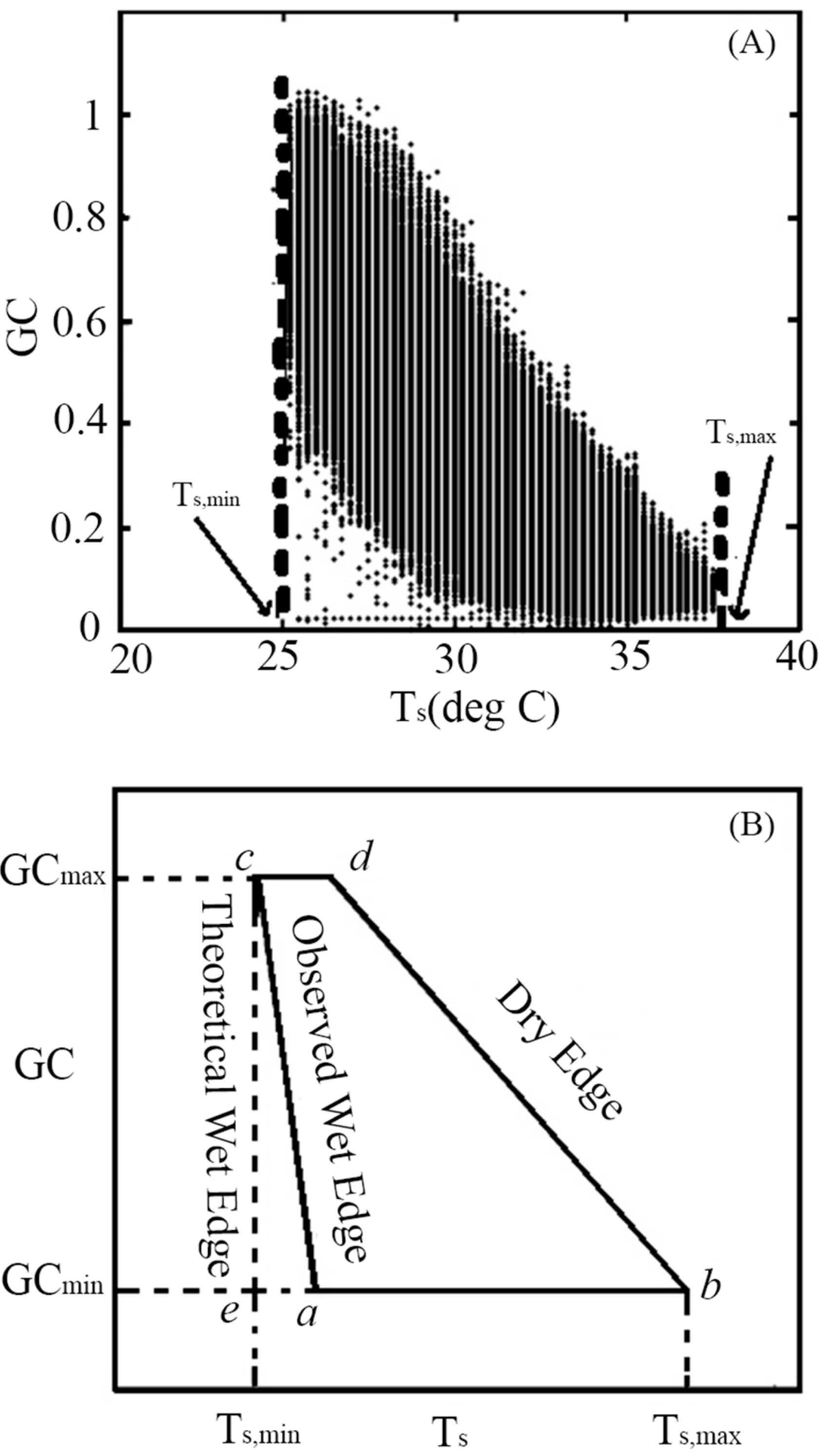
3.1. TIR–GC Space vs. Ts-GC Space

Plot of TIR as a function of GC for each image showed that the TIR-GC space is well defined in all cases (Figure 5). The thermal radiation rate decreases when the GC increases. From those plots we found that pixels in most of the scatter plots can form a trapezoid, indicating a very wide soil moisture condition range. In addition, this figure shows that the TIR-GC space has the same shape as the Ts-VI space.
Figure 5. Plots of GC values vs. TIR values for each image acquisition, along with corresponding plots of GC vs. Ts.
Remotesensing 07 02352 g005
Differences in the TIR range among acquisitions can largely be attributing to different atmospheric condition or amounts of irrigation or rainfall. This similarity between TIR-GC space and Ts-GC space means that TIR-GC space can be used in further steps to estimate soil moisture content. Figure 6 shows that how the points corresponding to TIRmax and TIRmin were defined for each TIR-GC scatterplot. This figure shows that TIRmax and TIRmin are well-defined for all cases. These values were used to normalize TIR values according to Equation (1).
Figure 6. Identification of TIRmax and TIRmin used to normalized TIR values in the TIR-GC scatterplot.
Remotesensing 07 02352 g006

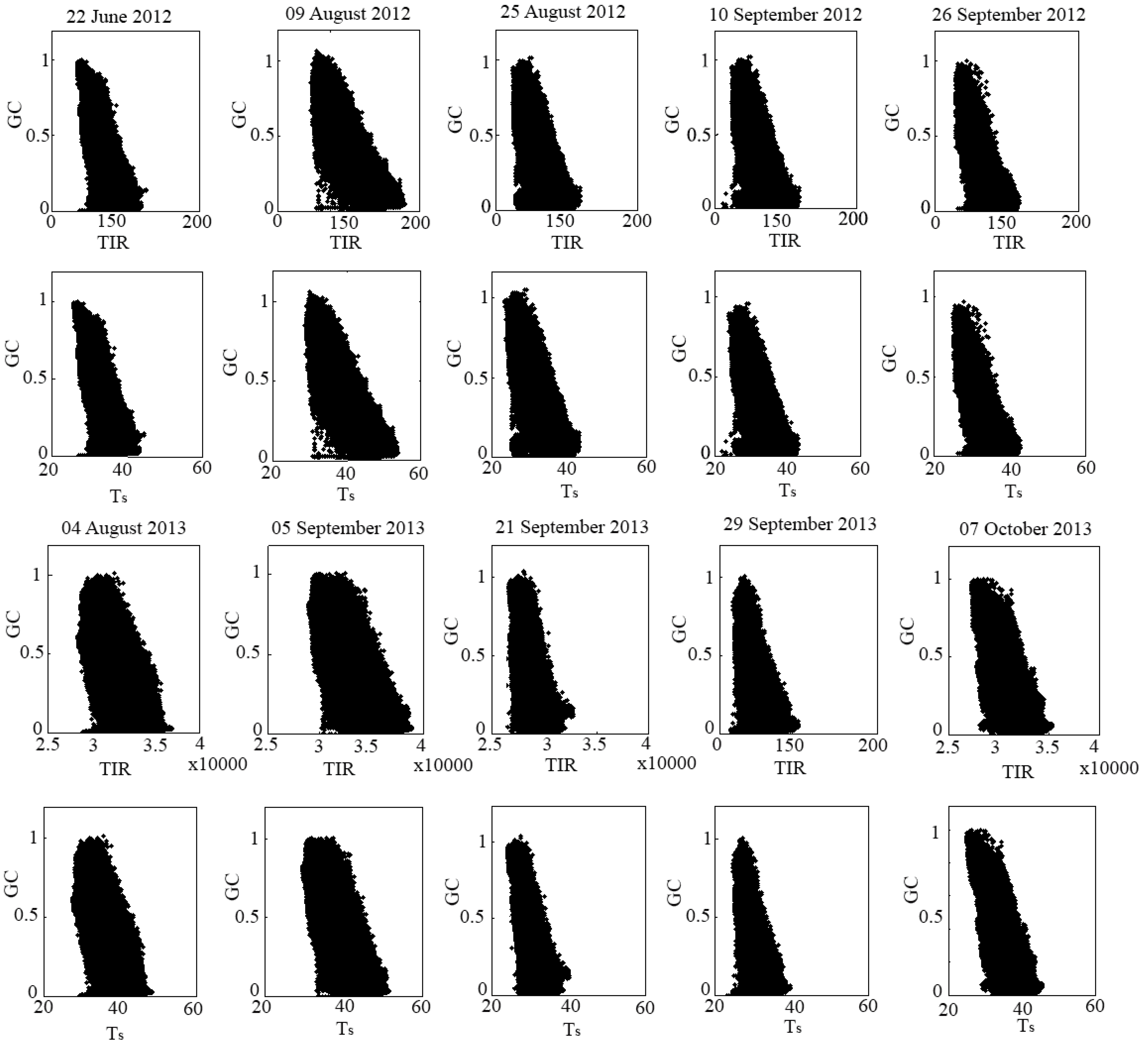
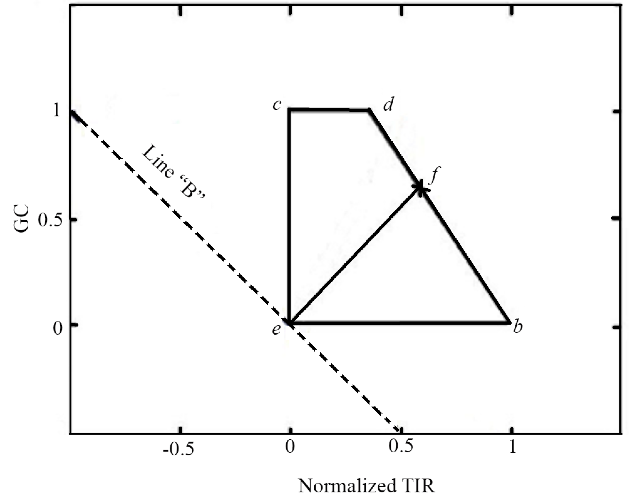
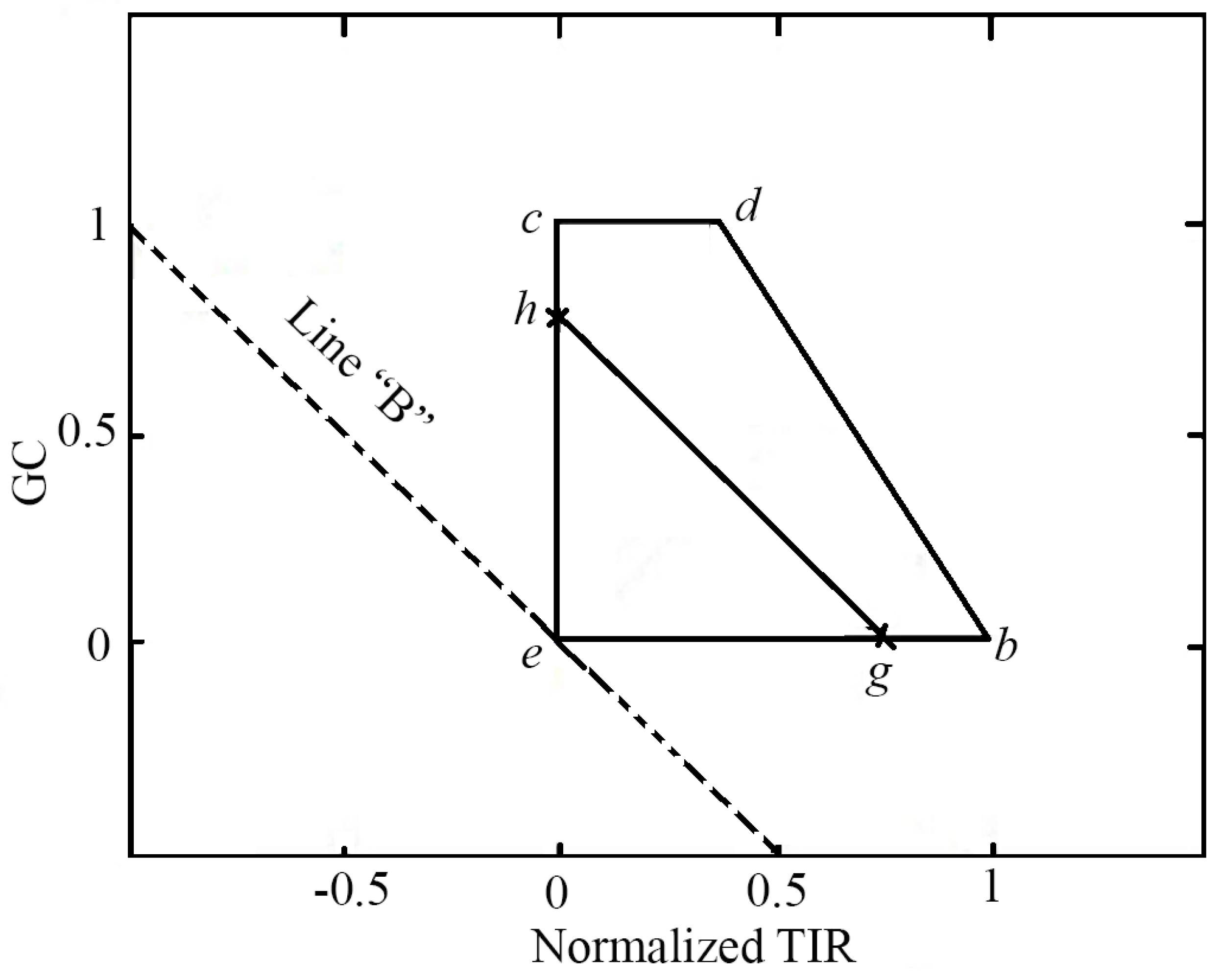
3.2. TIRnorm vs. Ts,norm

To compare TIRnorm vs. Ts,norm values, corresponding areas were selected in TIRnorm and Ts,norm images for each acquisition date. The average values of TIRnorm and Ts,norm for these selected areas were then calculated using the Region of Interest (ROI) tool in ENVI. The corresponding values of TIRnorm and Ts,norm were plotted in the overall TIRnorm-GC data space for each date. Figure 7 shows a comparison for 4 different dates (22 June 2012, 25 August 2012, 4 August 2013, 29 September 2013). These results suggest that TIRnorm and Ts,norm values for corresponding areas were in close agreement.
Figure 7. Comparison between TIRnorm and Ts,norm for the (A) 22 June 2012; (B) 25 August 2012; (C) 04 August 2013; (D) 29 September 2013 image acquisitions. The blue mark indicates the TIRnorm value while the red mark indicates the Ts,norm.
Remotesensing 07 02352 g007
A regression analysis of these data shows that the points tend to lie along the 1:1 line (Figure 8). The slope and intercept of the least-square linear regression fitted to the points is 1.01 and 0.005, respectively. Results of the Student’s t-test of the slope and intercept of this regression indicated that the slope was not significantly different from 1 (t = 0.338, 31 df, α = 0.05) and the intercept was not significantly different from 0 (t = 0.107, 31 df, α = 0.05) respectively. Thus, the regression line through these points is not significantly different from the 1:1 line. The Student’s t-test of the average TIRnorm and Ts,norm values indicates that these two values are not significantly different (t = −0.263, 64 df, α = 0.05), or in other words, these two values are almost the same. This suggests that, on average, TIRnorm can be used to estimate soil moisture instead of Ts,norm in the TIRnorm-GC space. The accuracy of the method that is used to calculate surface temperature from satellite imagery may change the correlation coefficient and the other statistical results that were presented. In addition the accuracy of defining the TIRmin and TIRmax position has effect on the results. This result was obtained in a part of Texas high plains that is flat area and there is no guarantee of obtaining the same result in different geographical conditions.
Figure 8. Simple linear regression between TIRnorm and Ts,norm for selected random fields.
Remotesensing 07 02352 g008

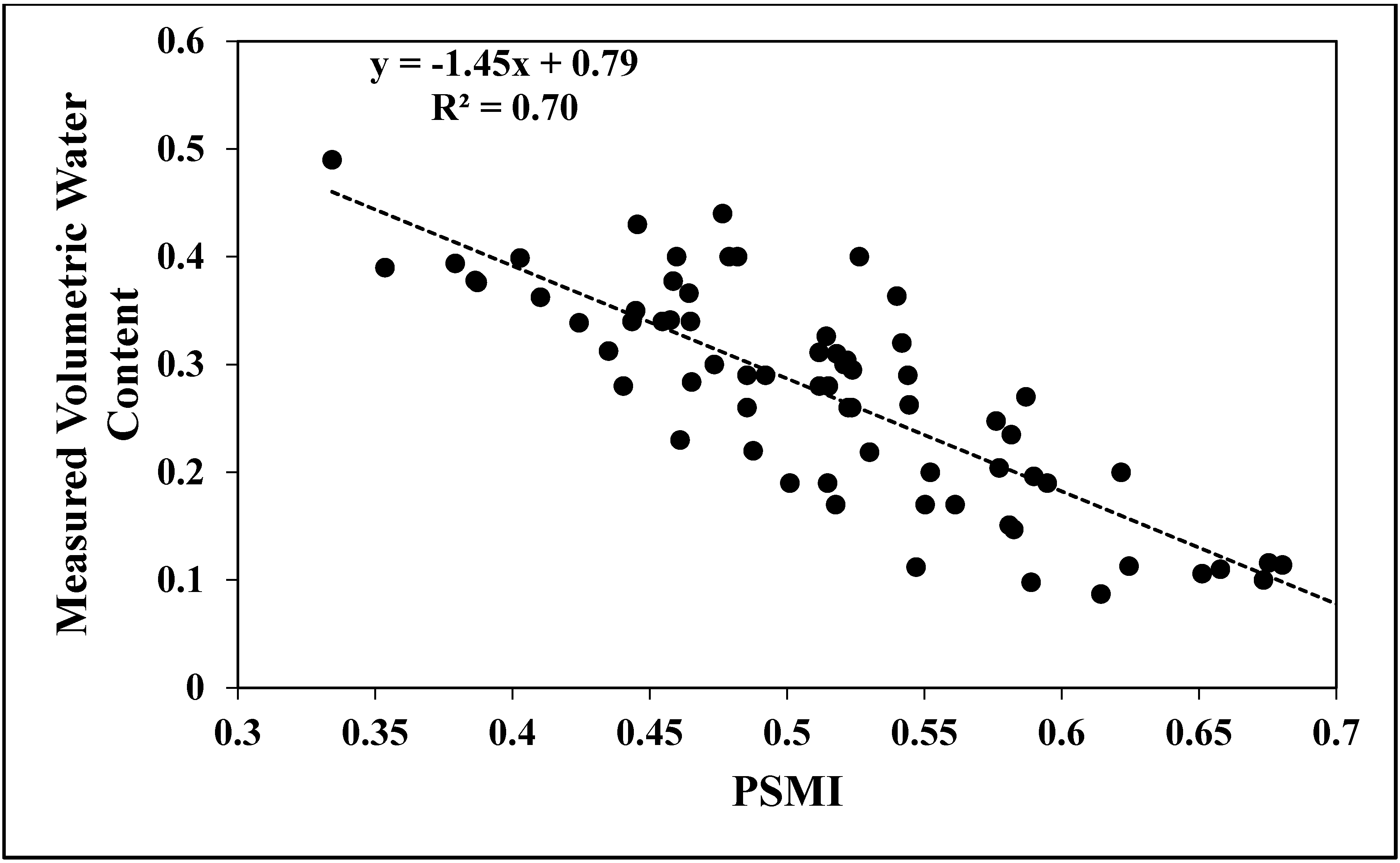
3.3. Comparison to Measured Soil Moisture

Figure 9 shows values of volumetric soil water content from measurements in the 18 study fields plotted vs. corresponding values of PSMI calculated from multispectral satellite image data using Equation (3). The solid line in the figure represents the 1:1 line. The solid line represents the simple linear regression fit to the points in the figure. This regression has the following equation,
VWC = 0.79 − 1.45 (PSMI)
in which VWC is volumetric water content and PSMI is the average value of the index for a field. Equation (4) explains that this regression line has a slope of 0.79 and a y-intercept of −1.45, and explains approximately 70% of the total variance in the data with an RMSE of 0.03 and Mean Bias Error (MBE) of 0.11. These results show that PSMI is highly correlated with soil moisture conditions in the field over a substantial range of soil moisture conditions (0.3 to 0.7 in Figure 9). The minus sign in Equation (4) means that there is a negative correlation between PSMI and soil moisture content. In the other words, higher value of PSMI is associated with lower amount of soil moisture content and lower value of PSMI is associated with higher soil moisture content. A great scale difference between the field measurement data and remote sensing data is an important factor that has a major impact on this comparison. Using satellite imagery with better spatial resolution can result in higher accuracy. In addition, the accuracy of soil moisture estimation from raw satellite data depends on the accuracy of GC and TIRnorm estimation from the scatter plots.
Figure 9. Simple linear regression between field measurements of volumetric soil water content and corresponding values of PSMI calculated from multispectral satellite image data.
Remotesensing 07 02352 g009
Monitoring soil moisture based on the space of TIRnorm-GC assumes that the meteorological parameters and land surface attributes are homogeneous, which simplifies the relationship between soil moisture and land surface thermal emission. In addition, it is assumed that the wet edge is a straight line, which can be considered a source of error.
While this relationship is purely statistical, it shows that remotely sensed quantities such as GC and TIR can be useful indicators of field conditions that are of interest to agronomists and producers, like soil moisture, but are often difficult or cost-prohibitive to directly measure over agricultural regions.
As an example of the utility of PMSI in assessing the spatial variation in field conditions across an agricultural region, Figure 10A,B shows maps of PSMI calculated on a pixel-by-pixel basis (using Equation (3)) for a 976 km2 square portion of the Texas High Plains on two separate dates. Figure 10A was constructed from Landsat-8 multispectral image data acquired on 4 August 2013, while Figure 10B was constructed from Landsat-8 multispectral image data acquired on 21 September 2013. In the figures, PSMI is color-coded to emphasize its variation across the landscape, and non-agricultural features (urban areas, water bodies), clouds, and cloud shadows have been masked in black. The information provided by PSMI is consistent with the known soil moisture conditions across the region. For the 4 August image (Figure 10A), PSMI is relatively low (indicated by green) in most of the irrigated fields, indicating that they are actively being irrigated—this is consistent with farming practices in the region at this time of peak crop growth. Surrounding dryland (non-irrigated) fields and pastures exhibit relatively high values of PSMI (indicated by orange and red), indicating less soil moisture content under strictly rainfed conditions.
Figure 10. PSMI maps constructed for two dates for a portion of the Texas High Plains. (A) PSMI map for 4 August 2013; (B) PSMI map for 21 September 2013. Green indicates low values of PSMI (high moisture), while orange and red indicates high values of PSMI (low moisture). Urban areas, water bodies, clouds and cloud shadows are masked in black.
Remotesensing 07 02352 g010
For the 21 September image (Figure 10B), most irrigation has been terminated so PSMI is higher in most of the fields that previously were irrigated. Image products such as these could be useful in monitoring regional soil moisture or drought conditions, and could provide input or calibration information for running models of crop growth and yield.

4. Conclusions

Surface soil moisture content is of great importance in closing hydrologic budgets, assessing soil plant water interactions and studying climate change. This study developed a new soil moisture index using raw image digital count (DC) to monitor the soil moisture condition. The raw thermal data (TIR) and ground cover (GC) evaluated directly from Landsat medium-resolution satellite imagery in the red, near-infrared and thermal infrared spectral bands were used to establish a trapezoidal space. The perpendicular distance from each pixel to a reference line that passed through the origin of this trapezoid was used to calculate the index. The greatest advantage of the Perpendicular Soil Moisture Index (PSMI) is that it substitutes the raw thermal radiation (TIR) for the surface temperature (Ts), which reduces expense and complexity in estimating the soil moisture. It means that PSMI can be evaluated on a pixel-by-pixel basis using raw image DC data without the need for conversion to radiance or reflectance or atmospheric calibration. A simple normalization was used to decrease the atmospheric effect and produce normalized distribution. This means the PSMI is more straightforward and less time-consuming than those that use Ts to estimate soil moisture content.
Using measurements of volumetric soil water content obtained from 18 agricultural fields in the Texas High plains over 2 years, statistical analysis showed that PSMI is highly and negatively correlated with soil moisture content (R2 = 0.703). Although the number of field measurements was limited, they allowed the confirmation that the PSMI provides, as stated in the theoretical design, correct information on soil moisture condition. It is recommended, however, that the PSMI be validated further with more field measurements in additional ecosystems.
PSMI was used to construct maps showing the spatial distribution of soil moisture conditions over an agricultural region in which patterns of high and low PSMI were consistent with what would be expected from known crop management practices. Changes in the spatial distribution of PSMI over time were consistent with changes in irrigation in the region.
We acknowledge that the soil moisture monitored in the upper 5 cm or less is of limited use for hydrologic and agricultural applications, which is primarily constrained by remote sensing. The greatest advantage of remote sensing is its ability to continuously spatially monitor large areas, which cannot occur with a limited number of ground-based stations. If the vertical soil moisture profile can be known a priori, one can extrapolate the remote sensing based soil moisture in the upper soil to the deep layer. Additional testing with measured soil moisture data will help assess the accuracy of this approach in estimating soil moisture, and identify its possible limitations. However, PSMI appears to be a potentially useful indicator of soil moisture that could find practical use in a range of applications, such as regional water resource monitoring and irrigation scheduling.

Acknowledgments

The authors would like to thank the Texas Alliance for Water Conservation (TAWC) Demonstration Project, funded through the Texas Water Development Board, for the resources to conduct this study.

Author Contributions

Sanaz Shafian and Stephan J. Maas conceived and designed the experiments; Sanaz Shafian collected data, analyzed the data, developed the model and wrote the paper; Stephan J. Maas contributed developing model and writing the paper.

Conflicts of Interest

The authors declare no conflict of interest.

References

  1. Rajan, N.; Maas, S.J.; Kathilankal, J.C. Estimating crop water use of cotton in the Southern High Plains. Agron. J. 2010, 102, 1641–1651. [Google Scholar] [CrossRef]
  2. Payero, J.O.; Tarkalson, D.D.; Irmak, S.; Davison, D.; Petersen, J.L. Effect of irrigation amounts applied with subsurface drip irrigation on corn evapotranspiration, yield, water use efficiency, and dry matter production in a semiarid climate. Agric. Water Manag. 2008, 95, 895–908. [Google Scholar] [CrossRef]
  3. Ko, J.; Piccinni, G. Corn yield responses under crop evapotranspiration-based irrigation management. Agric. Water Manag. 2009, 96, 799–808. [Google Scholar] [CrossRef]
  4. Lobell, D.B.; Gourdji, S.M. The influence of climate change on global crop productivity. Plant Physiol. 2012, 160, 1686–1697. [Google Scholar] [CrossRef] [PubMed]
  5. Hatfield, J.L.; Boote, K.J.; Kimball, B.A.; Ziska, L.H.; Izaurralde, R.C.; Ort, D.; Thomson, A.M.; Wolfe, D. Climate impacts on agriculture: Implications for crop production. Agron. J. 2011, 103, 351–370. [Google Scholar] [CrossRef]
  6. Hemakumara, M.H. Aggregation and Disaggregation of Soil Moisture Measurements. Ph.D. Dissertation, The University of Newcastle, Newcastle, NSW, Australia, 2007. [Google Scholar]
  7. Goward, S.N.; Waring, R.H.; Dye, D.G.; Yang, J. Ecological remote sensing at Otter: Macro scale satellite observations. Ecol. Appl. 1994, 4, 322–343. [Google Scholar] [CrossRef]
  8. Merlin, O.; Rüdiger, C.; Bitar, A.A.; Richaume, P.; Walker, J.P.; Kerr, Y.H. Disaggregation of SMOS soil moisture in Southeastern Australia. IEEE Trans. Geosci. Remote Sens. 2012, 50, 1556–1571. [Google Scholar] [CrossRef] [Green Version]
  9. Verstraeten, W.W.; Veroustraete, F.; van der Sande, C.J.; Grootaers, I.; Feyen, J. Soil moisture retrieval using thermal inertia, determined with visible and thermal space borne data, validated for European forests. Remote Sens. Environ. 2006, 101, 299–314. [Google Scholar] [CrossRef]
  10. Wagner, W.; Naeimi, V.; Scipal, K.; Jeu, R.D.; Fernandez, J.M. Soil moisture from operational meteorological satellite. Hydrogeol. J. 2007, 15, 121–131. [Google Scholar] [CrossRef]
  11. Courault, D.; Seguin, B.; Olioso, A. Review on estimation of evapotranspiration from remote sensing data: From empirical to numerical modelling approaches. Irrig. Drain. Syst. 2005, 19, 223–249. [Google Scholar] [CrossRef]
  12. Moran, M.S.; Clarke, T.R.; Inoue, Y.; Vidal, A. Estimating crop water deficit using the relation between surface-air temperature and spectral vegetation index. Remote Sens. Environ. 1994, 49, 246–263. [Google Scholar] [CrossRef]
  13. Goward, S.N.; Xue, Y.; Czajkowski, K.P. Evaluating land surface moisture conditions from the remotely sensed temperature/vegetation index measurements: An exploration with the simplified simple biosphere model. Remote Sens. Environ. 2002, 79, 225–242. [Google Scholar] [CrossRef]
  14. Patel, N.R.; Anapashsha, R.; Kumar, S.; Saha, S.K.; Dadhwal, V.K. Assessing potential of MODIS derived temperature/vegetation condition index (TVDI) to infer soil moisture status. Int. J. Remote Sens. 2009, 30, 23–39. [Google Scholar] [CrossRef]
  15. Rahimzadeh, B.P.; Berg, A.A.; Champagne, C.; Omasa, K. Estimation of soil moisture using optical/thermal infrared remote sensing in the Canadian Prairies. ISPRS J. Photogramm. Remote Sens. 2013, 83, 94–103. [Google Scholar] [CrossRef]
  16. Carlson, T.N. An overview of the “triangle method” for estimating surface evapotranspiration and soil moisture from satellite imagery. Sensors 2007, 7, 1612–1629. [Google Scholar] [CrossRef]
  17. Carlson, T.N.; Dodd, J.K.; Benjamin, S.G.; Cooper, J.N. Satellite estimation of surface energy balance, moisture availability and thermal inertia. J. Appl. Meteorol. 1981, 20, 67–87. [Google Scholar] [CrossRef]
  18. Soliman, A.; Heck, R.J.; Brenning, A.; Brown, R.; Miller, S. Remote sensing of soil moisture in vineyards using airborn and ground-based thermal inertia data. Remote Sens. 2013, 5, 3729–3748. [Google Scholar] [CrossRef]
  19. Hain, C.R.; Mecikalski, J.R. Retrieval of an available water-based soil moisture proxy from thermal infrared remote sensing. Part I: methodology and validation. J. Hydrometeorol. 2009, 10, 665–683. [Google Scholar] [CrossRef]
  20. Price, J.C. The potential of remotely sensed data to infer surface soil moisture and evaporation. Water Resour. Res. 1980, 16, 787–795. [Google Scholar] [CrossRef]
  21. Fang, B.; Lakshmi, V. Soil moisture at watershed scale: Remote sensing techniques. J. Hydrol. 2014, 516, 258–272. [Google Scholar] [CrossRef]
  22. Kasischke, E.S.; Bourgeau-Chavez, L.L.; Johnstone, J.F. Assessing spatial and temporal variations in surface soil moisture in fire-disturbed black spruce forests in Interior Alaska using space borne synthetic aperture radar imagery—Implications for post-fire tree recruitment. Remote Sens. Environ. 2007, 108, 42–58. [Google Scholar] [CrossRef]
  23. Dupigny-Giroux, L.L. Using air MISR data to explore moisture-driven land use–land covers variations at the Howland Forest, Maine-A case study. Remote Sens. Environ. 2007, 107, 376–384. [Google Scholar] [CrossRef]
  24. Chen, C.F.; Valdez, M.C.; Chang, N.B.; Chang, L.Y.; Yuan, P.Y. Monitoring spatiotemporal surface soil moisture variations during dry seasons in central America with multisensor cascade data fusion. IEEE J. Sel. Top. Appl. Earth Obs. Remote Sens. 2014, 7, 1939–1404. [Google Scholar]
  25. Chen, X.; Su, Y.; Li, Y.; Han, L.; Liao, J.; Yang, S. Retrieving China’s surface soil moisture and land surface temperature using AMSR-E brightness temperatures. Remote Sens. Lett. 2014, 7, 662–671. [Google Scholar] [CrossRef]
  26. Petropoulos, G.; Carlson, T.N.; Wooster, M.J.; Islam, S. A review of Ts/VI remote sensing based methods for the retrieval of land surface energy fluxes and soil surface moisture. Prog. Phys. Geogr. 2009, 33, 224–250. [Google Scholar] [CrossRef]
  27. Wang, K.; Li, Z.; Cribb, M. Estimation of evaporative fraction from a combination of day and night land surface temperatures and NDVI: A new method to determine the Priestley-Taylor parameter. Remote Sens. Environ. 2006, 102, 293–305. [Google Scholar] [CrossRef]
  28. Wan, Z.; Wang, P.; Li, X. Using MODIS land surface temperature and Normalized Difference Vegetation Index products for monitoring drought in the Southern Great Plains, USA. Int. J. Remote Sens. 2004, 25, 61–72. [Google Scholar] [CrossRef]
  29. Jackson, R.D.; Idso, D.B.; Reginato, R.J.; Pinter, P.J. Canopy temperature as a crop water stress indicator. Water Resour. Res. 1981, 17, 1133–1138. [Google Scholar] [CrossRef]
  30. Yuan, W.; Liu, S.; Yu, G.; Bonnefond, J.M.; Chen, J.; Davis, K.; Desai, A.R.; Goldstein, A.H.; Gianelle, D.; Rossi, F.; et al. Global estimates of evapotranspiration and gross primary production based on MODIS and global meteorology data. Remote Sens. Environ. 2010, 114, 1416–1431. [Google Scholar] [CrossRef]
  31. Goward, S.N.; Hope, A.S. Evapotranspiration from combined reflected solar and emitted terrestrial radiation: Preliminary FIFE results from AVHRR data. Adv. Space Res. 1989, 9, 239–249. [Google Scholar] [CrossRef]
  32. Yang, X.; Wu, J.J.; Shi, P.J.; Yan, F. Modified triangle method to estimate soil moisture with Moderate Resolution Imaging Spectroradiometer (MODIS) products. Int. Arc. Photogramm. 2008, 37, 555–560. [Google Scholar]
  33. Carlson, T.N. Triangle models and misconceptions. Int. J. Remote Sens. Appl. 2013, 3, 155–158. [Google Scholar]
  34. Zhang, D.; Tang, R.; Zhao, W.; Tang, B.; Wu, H.; Shao, K.; Li, Z.L. Surface soil water content estimation from thermal remote sensing based on the temporal variation of land surface temperature. Remote Sens. 2014, 6, 3170–3187. [Google Scholar] [CrossRef] [Green Version]
  35. Stisen, S.; Sandholt, I.; Norgaard, A.; Fensholt, R.; Jensen, K.H. Combining the triangle method with thermal inertia to estimate regional evapotranspiration—Applied to MSG SEVIRI data in the Senegal River basin. Remote Sens. Environ. 2008, 112, 1242–1255. [Google Scholar] [CrossRef]
  36. Tang, R.L.; Li, Z.-L.; Chen, K.S. Validating MODIS-derived land surface evapotranspiration with in situ measurements at two AmeriFlux sites in a semiarid region. J. Geophys. Res. 2011, 116. [Google Scholar] [CrossRef]
  37. Tang, R.L.; Li, Z.-L.; Chen, K.S.; Zhu, Y.; Liu, W. Verification of land surface evapotranspiration estimation from remote sensing spatial contextual information. Hydrol. Process 2012, 26, 2283–2293. [Google Scholar] [CrossRef]
  38. Cai, G.; Xue, Y.; Hu, Y.; Wang, Y.; Guo, J.; Luo, Y.; Wu, C.; Zhong, S.; Qi, S. Soil moisture retrieval from MODIS data in Northern China Plain using thermal inertia model. Int. J. Remote Sens. 2007, 28, 3567–3581. [Google Scholar] [CrossRef]
  39. Carlson, T.N.; Arthur, S.T. The impact of land use—Land cover changes due to urbanization on surface microclimate and hydrology: A satellite perspective. Glob. Planet. Chang. 2000, 25, 49–65. [Google Scholar] [CrossRef]
  40. Wang, W.; Huang, D.; Wang, X.G.; Liu, Y.R.; Zhou, F. Estimate soil moisture using trapezoidal relationship between remotely sensed land surface temperature and vegetation index. Hydrol. Earth Syst. Sci. Discuss. 2010, 7, 8703–8740. [Google Scholar] [CrossRef]
  41. Jiang, L.; Islam, S.A.; Guo, W.; Jutla, A.S.; Senarath, S.U.S.; Ramsay, B.H.; Eltahir, E. A satellite-based daily actual evapotranspiration estimation algorithm over South Florida. Glob. Planet. Chang. 2009, 67, 62–77. [Google Scholar] [CrossRef]
  42. Yang, Y.; Scott, R.L.; Shang, S. Modeling evapotranspiration and its partitioning over a semiarid shrub ecosystem from satellite imagery: A multiple validation. J. Appl. Remote Sens. 2013, 7, 073495. [Google Scholar] [CrossRef]
  43. Long, D.; Singh, V.P. A two-source trapezoid model for evapotranspiration (TTME) from satellite imagery. Remote Sens. Environ. 2012, 121, 370–388. [Google Scholar] [CrossRef]
  44. Yang, Y.; Shang, S. A hybrid dual-source scheme and trapezoid framework–based evapotranspiration model (HTEM) using satellite images: Algorithm and model test. J. Geophys. Res.: Atmos. 2013, 118, 2284–2300. [Google Scholar] [CrossRef]
  45. Jiang, L.; Islam, S.A. Methodology for estimation of surface evapotranspiration over large areas using remote sensing observations. Geophys. Res. Lett. 1999, 26, 2773–2776. [Google Scholar] [CrossRef]
  46. Jiang, L.; Islam, S.A. Estimation of surface evaporation map over Southern Great Plains using remote sensing data. Water Resour. Res. 2001, 37, 329–340. [Google Scholar] [CrossRef]
  47. Sandholt, I.; Rasmussen, K.; Andersen, J. A simple interpretation of the surface temperature/vegetation index space for assessment of soil moisture status. Remote Sens. Environ. 2002, 79, 213–224. [Google Scholar] [CrossRef]
  48. Jiang, L.; Islam, S.A. An intercomparison of regional heat flux estimation using remote sensing data. Int. J. Remote Sens. 2003, 24, 2221–2236. [Google Scholar] [CrossRef]
  49. Mallick, K.; Bhattacharya, B.K.; Patel, N.K. Estimating volumetric surface moisture content for cropped soils using a soil wetness index based on surface temperature and NDVI. Agric. For. Meteorol. 2009, 149, 1327–1342. [Google Scholar] [CrossRef]
  50. Tadesse, T.; Brown, J.; Hayes, M. A new approach for predicting drought-related vegetation stress: Integrating satellite, climate, and biophysical data over the U.S. central plains. ISPRS J. Photogram. Remote Sens. 2005, 59, 244–253. [Google Scholar] [CrossRef]
  51. Li, Z.L.; Tang, R.; Wan, Z.; Bi, Y.; Zhou, C.; Tang, B.; Yan, G.; Zhang, X. A review of current methodologies for regional evapotranspiration estimation from remotely sensed data. Sensors 2009, 9, 3801–3853. [Google Scholar] [CrossRef] [PubMed]
  52. Maas, S.J.; Rajan, N. Estimating ground cover of field crops using medium-resolution multispectral satellite imagery. Agron. J. 2008, 100, 320–327. [Google Scholar] [CrossRef]
  53. Moran, S. Crop Stress. In Encyclopedia Earth Sciences Series; Springer: New York, NY, USA, 2014; pp. 88–91. [Google Scholar]
  54. Shafian, S.; Maas, S.J. Improvement of the Trapezoid method using raw Landsat image digital count data for soil moisture estimation in the Texas (USA) High Plains. Sensors 2015, 15, 1925–1944. [Google Scholar] [CrossRef] [PubMed]
  55. Shafian, S. Estimation of soil moisture status in the Texas high plains using remote sensing. Ph.D. Dissertation, Texas Tech University, Lubbock, TX, USA, 2014. [Google Scholar]
  56. Richardson, A.J.; Wiegand, C.L. Distinguishing vegetation from soil background. Photogram. Eng. Remote Sens. 1977, 43, 1541–1552. [Google Scholar]
  57. USGS science for a changing world. Available online: http://earthexplorer.usgs.gov/ (accessed on 18 August 2014).
  58. Chander, G.; Markham, B. Revised Landsat-5 TM radiometric calibration procedures and post calibration dynamic ranges. IEEE Trans. Geosci. Remote Sens. 2003, 41, 2674–2677. [Google Scholar] [CrossRef]
  59. Bastiaanssen, W.G.M.; Menenti, M.; Feddes, A.R.; Holtslag, A.M. A remote sensing Surface Energy Balance Algorithm for Land (SEBAL). 1. Formulation. J. Hydrol. 1998, 212–213, 198–212. [Google Scholar] [CrossRef]

