1. Introduction
In the past 50 years, while cities have experienced population growth and land consumption, the pressures on vital ecosystem functions have escalated rapidly [
1,
2]. Urbanization, which means a population shift from rural to urban areas, is often accompanied by urban expansion and land use change. To interpret the land consumption pressures, the impact of urbanization has been documented in the growing literature on the urban–rural gradient, which shows consistent changes in species richness and species composition [
3,
4,
5]. With worldwide land cover change, biogeochemical cycles, hydrologic systems, and climate and biodiversity change driven by urbanization, increasing numbers of ecologists have accepted that urban areas are hot spots that drive environmental change on multiple scales [
6]. These hot spots are estimated not only to be current threats for ecosystems but also will probably last for a long period in developing nations. The global urban population will reach 5 billion by 2030 [
7] and will increase by 2.7 billion, nearly doubling today’s urban population of 3.4 billion by 2050 [
8], which indicates that the dramatic urbanization phenomenon will continue. Therefore, the threat of changes in biodiversity with an increase in global urbanization is a concern that needs to be brought to the foreground [
9].
The total vegetation in urban and suburban areas is an important indicator of urbanization pressure on biodiversity, because plants can be lost during either the initial habitat transformation or the landscape fragmentation processes [
5]. Vegetation degradation, which means a reduction in the available biomass, often represents as a decline in the vegetative ground cover. Vegetation degradation triggered by a change of land cover to impervious surfaces in urban areas may result in eco-environmental threats with net primary production reduction and surface temperature variation [
10,
11]. However, some opposite perspectives have recently put forward a different relation, which suggest some urbanization factors can enhance urban vegetation activity [
12]. The plant growth in urban areas might be promoted by warmer temperature and greater tropospheric CO
2 concentration [
13,
14]. Because the value of urban ecosystem services has been deeply rooted in landscape management [
15], green infrastructure investments are supported and some negative urbanization effects are mitigated by landscape planning [
16,
17]. On balance, the interconnection between vegetation degradation and urbanization seems to be a complex and nonlinear system [
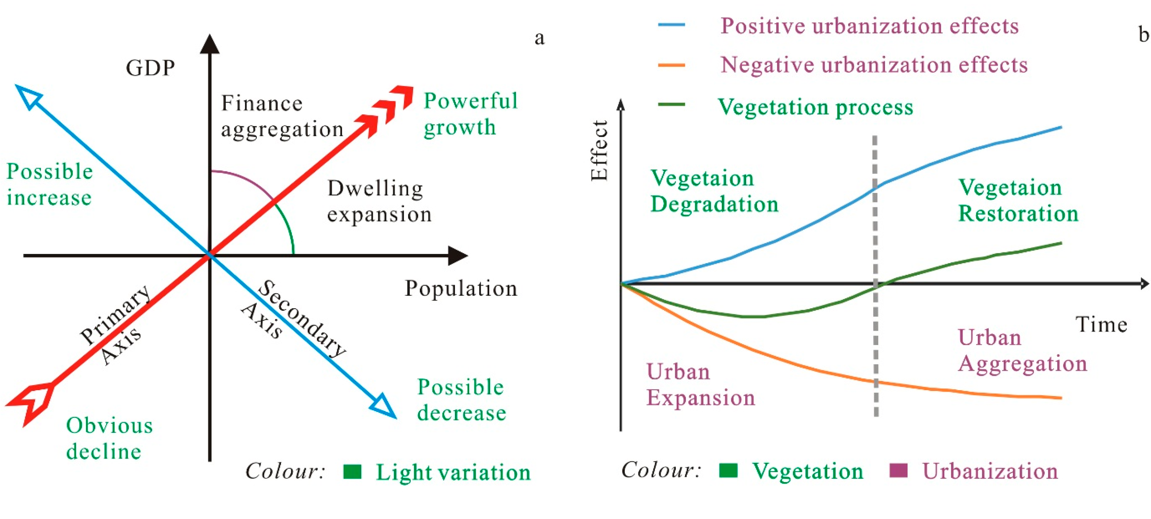
12].
Accordingly, a hypothesis can be proposed that the spatiotemporal relations between urbanization and vegetation degradation are diversified and may relate to the stage of urbanization and geographical location. However, a systematic evaluation of the spatiotemporal trends of vegetation activities across multiple cities over large areas is still lacking [
12]. The Normalized Difference Vegetation Index (NDVI) has been adopted as an effective index for describing the dynamics of urban vegetation [
18,
19]. As a remote sensing index, NDVI can indirectly estimate gross and net primary productivity, biomass, and green leaf area in a variety of grassland and forest ecosystems [
20,
21,
22,
23,
24]. If a regular distribution of NDVI variation rate on the urban–rural gradient exists, the landscape is likely to experience a negative effect related to urbanization on vegetation. Therefore, in this article, the NDVI variation rate is adopted as a vegetation degradation indicator that can be extracted across multiple cities over large areas.
The Defense Meteorological Satellite Program (DMSP)/Operational Line-Scan System (OLS) nighttime stable light data (NTL) s been demonstrated to be an effective data source for mapping urban expansion and urbanization dynamics at a large spatial scale [
25,
26,
27,
28,
29,
30]. NTL not only can be applied to urban area extraction, but also widely reflect population density, economic activity, and energy use in an urban area [
31,
32,
33,
34,
35]. Therefore, the image’s digital number (DN) may take on a growing trend in rapidly urbanized areas of developing countries. However, the DN may seem relatively stable in the core urban areas of developed countries, because of saturation at the highest value. To find the differentiation of nighttime light change among various cities, urbanization trends derived from DN were calculated and compared with the NDVI variation rates in the same geographical extent.
In light of the hypothesis that the spatiotemporal relations between urbanization and vegetation degradation should show differences, the study presented here contains four major parts. (a) To develop a simplified calibration method on NTL series to extract the urbanization area of the world’s metropolises; (b) To detect the variation trends of vegetation and urbanization by Theil-Sen regression [
36,
37]; (c) To classify the metropolises and differentiate between different relations in the variation trends; (d) To discuss the impact of human factors on vegetation changes in urbanization.
3. Methods
NTL data cannot be used directly to extract the dynamics of urbanization, because the DN value of NTL data is the average value from archived data without any on-board calibration [
30,
43]. To confirm the continuity and comparability of NTL data, former research was consulted, and the intercalibration method was improved to correct the data systematically for urbanization detection [
30,
42,
43,
44]. In this article, a simplified intercalibration method was used before the DN yearly series was generated. In the trend judgment part, the former research indicated that the unbiased predictor of the Theil-Sen approach was suggested as a potential replacement for ordinary least squares for linear regression in remote sensing applications [
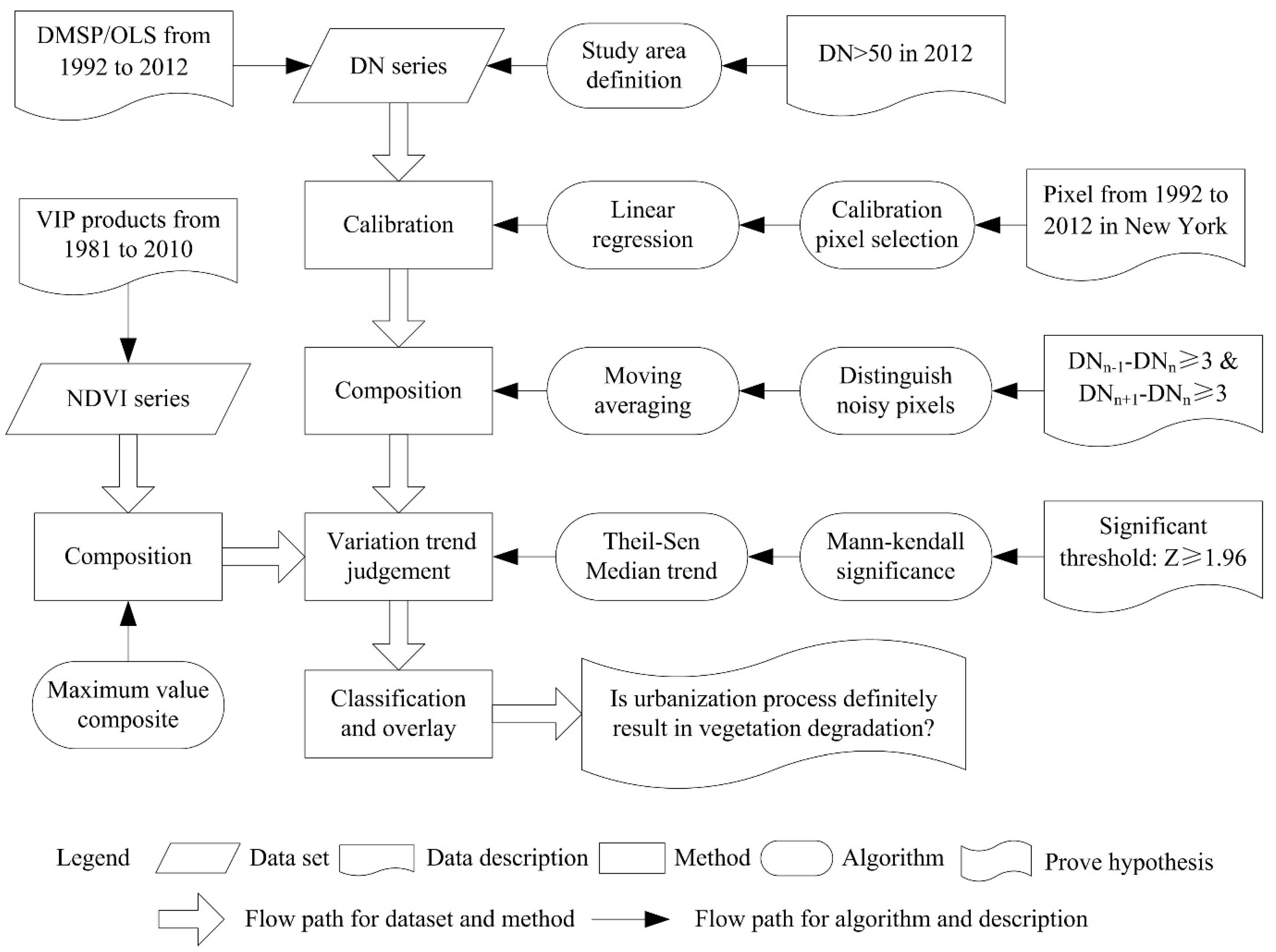
45]. Therefore, the Theil-Sen median trend is used in this article to quantify the variation of NDVI and DN. Finally, in the overlay analysis part, after the trend maps are overlaid and the different urbanization types are classified, we can determine whether the urbanization process definitely results in vegetation degradation. This procedure can be simplified as in
Figure 2.
Figure 2.
The flowchart for this research.
Figure 2.
The flowchart for this research.
3.1. Calibration and Composition of NTL
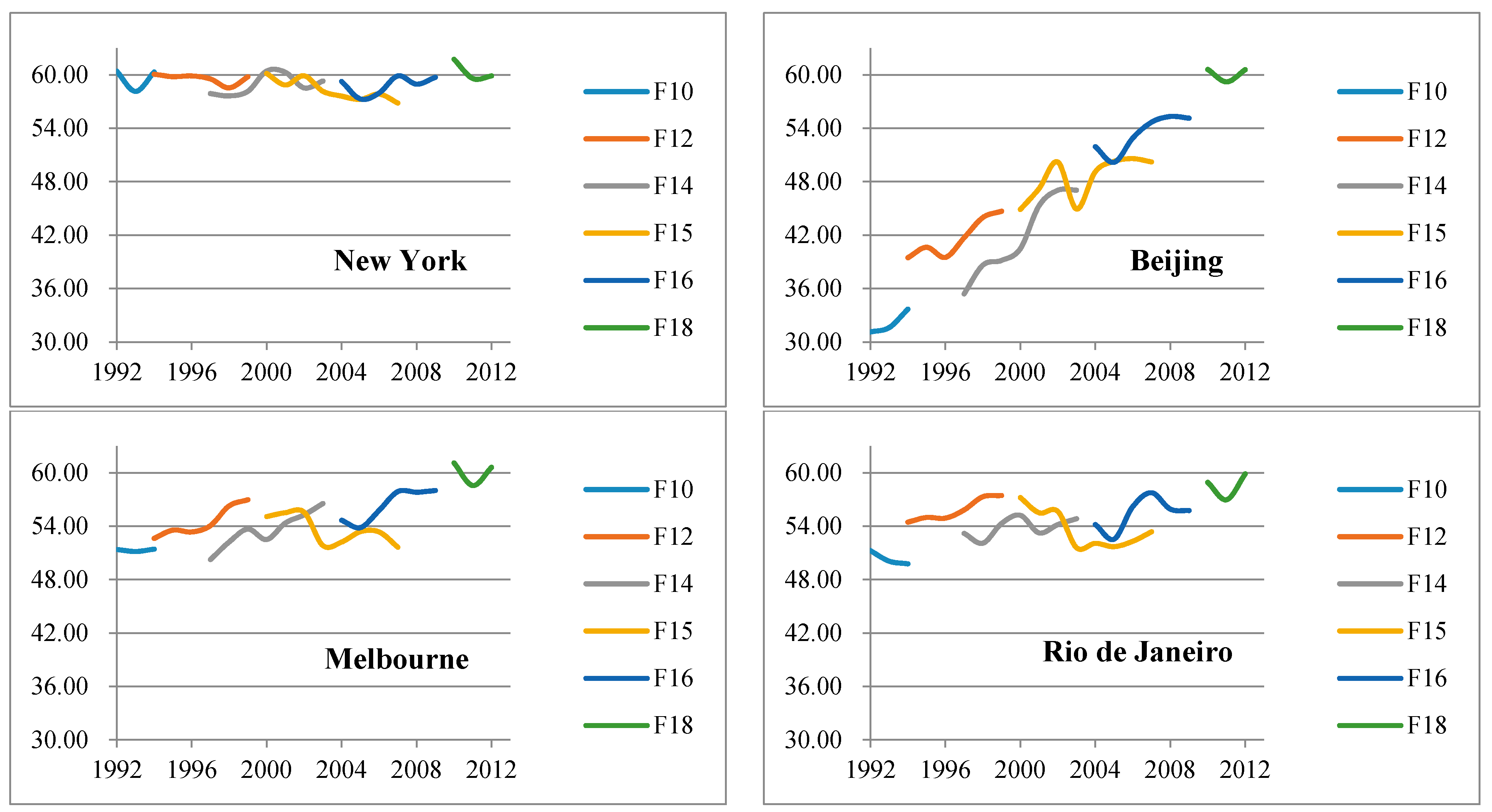
DN values from the same satellite for different years or from different satellites for the same year often show discrepancies or abnormal fluctuations, which are partly attributable to unstable spill light [
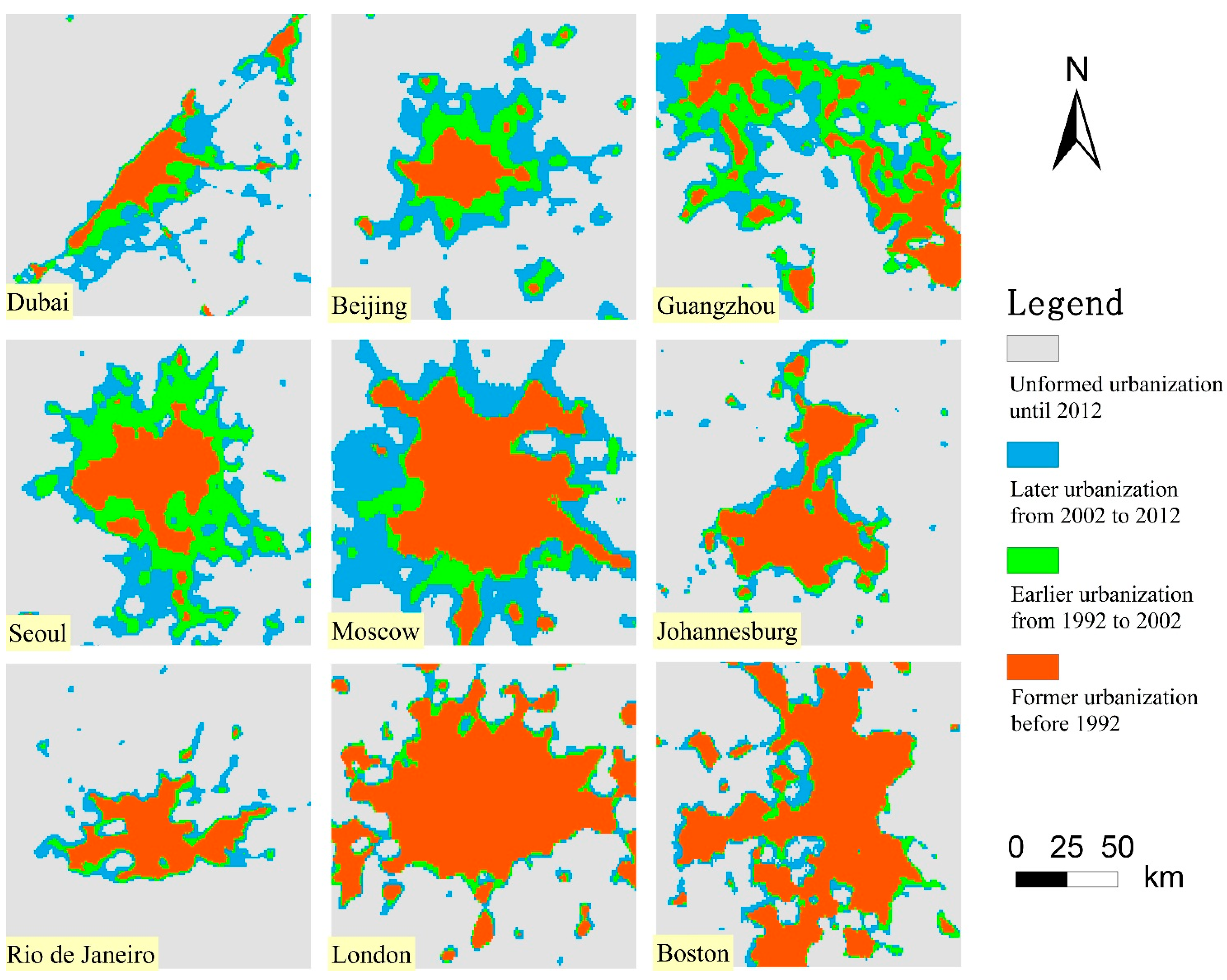
30]. As
Figure 3 shows, the post-urbanization stage for New York and swift urbanization stage for Beijing are evident. However, in Melbourne and Rio de Janeiro, the trend is in fluctuation and is confused because increasing and decreasing trends may appear during the same period from different satellites. To make the result credible, intercalibration is needed to detect the brightness changes across the time series [
46]. Faced with this obstacle, Elvidge
et al. (2009, 2014) developed a second-order regression model, with F121999 used as the reference composite and with Sicily chosen as the reference region [
43,
46]. The form of the calculation is Y = C
0 + C
1X + C
2X
2, and calculated values that run beyond 63 are truncated at 63. Although some issues are debatable, it is generally reasonable to be focused on the whole statistical value rather than particular pixels [
33].
After comparing the 50 metropolitan areas, we found the DN in New York most stable. Because the spatial extent of urbanization has been extracted by F182012, and most of the pixel values in this extent are higher than 30 in the former years, F182012 is used as the reference composite, and DN > 30 in New York is chosen as the reference region. Also, because we only deal with data ranging from 30 to 63 instead of 0–63, a second-order regression model may be insufficient. The inflection point in the quadratic curve may not appear in this half of the data range. In fact, we find no significant difference between the
R2 from the second-order regression model and the first-order regression model. Thus we simplified the calculation as Y = aX + b, where X means the DN in the NTL data set and Y means the DN after intercalibration. The intercalibration applied on the basis of the offsets and coefficients is listed in
Table 3.
Figure 3.
Examples of DN values in the urbanization area from different satellites before calibration during 1992–2012.
Figure 3.
Examples of DN values in the urbanization area from different satellites before calibration during 1992–2012.
Table 3.
Coefficients of the simplified linear regression models for NTL from 1992 to 2012.
Table 3.
Coefficients of the simplified linear regression models for NTL from 1992 to 2012.
| Satellite | Year | a | b | R2 | Satellite | Year | a | b | R2 |
|---|
| F10 | 1992 | 0.50 | 26.61 | 0.74 | F15 | 2000 | 0.57 | 23.28 | 0.83 |
| 1993 | 0.48 | 28.80 | 0.75 | 2001 | 0.64 | 19.89 | 0.84 |
| 1994 | 0.54 | 23.70 | 0.72 | 2002 | 0.70 | 15.93 | 0.87 |
| F12 | 1994 | 0.52 | 26.46 | 0.82 | 2003 | 0.52 | 27.78 | 0.88 |
| 1995 | 0.60 | 21.64 | 0.79 | 2004 | 0.50 | 29.38 | 0.89 |
| 1996 | 0.63 | 19.66 | 0.81 | 2005 | 0.51 | 29.03 | 0.88 |
| 1997 | 0.52 | 26.30 | 0.77 | 2006 | 0.46 | 32.07 | 0.92 |
| 1998 | 0.53 | 26.38 | 0.79 | 2007 | 0.44 | 33.15 | 0.88 |
| 1999 | 0.73 | 13.71 | 0.82 | F16 | 2004 | 0.51 | 27.41 | 0.82 |
| F14 | 1997 | 0.44 | 32.16 | 0.84 | 2005 | 0.50 | 29.57 | 0.90 |
| 1998 | 0.47 | 31.24 | 0.86 | 2006 | 0.53 | 27.54 | 0.89 |
| 1999 | 0.49 | 29.30 | 0.87 | 2007 | 0.71 | 16.16 | 0.89 |
| 2000 | 0.84 | 7.65 | 0.88 | 2008 | 0.55 | 25.79 | 0.89 |
| 2001 | 0.62 | 20.32 | 0.83 | 2009 | 0.65 | 18.75 | 0.84 |
| 2002 | 0.51 | 27.24 | 0.79 | F18 | 2010 | 1.21 | −15.91 | 0.91 |
| 2003 | 0.62 | 21.21 | 0.87 | 2011 | 0.56 | 23.71 | 0.76 |
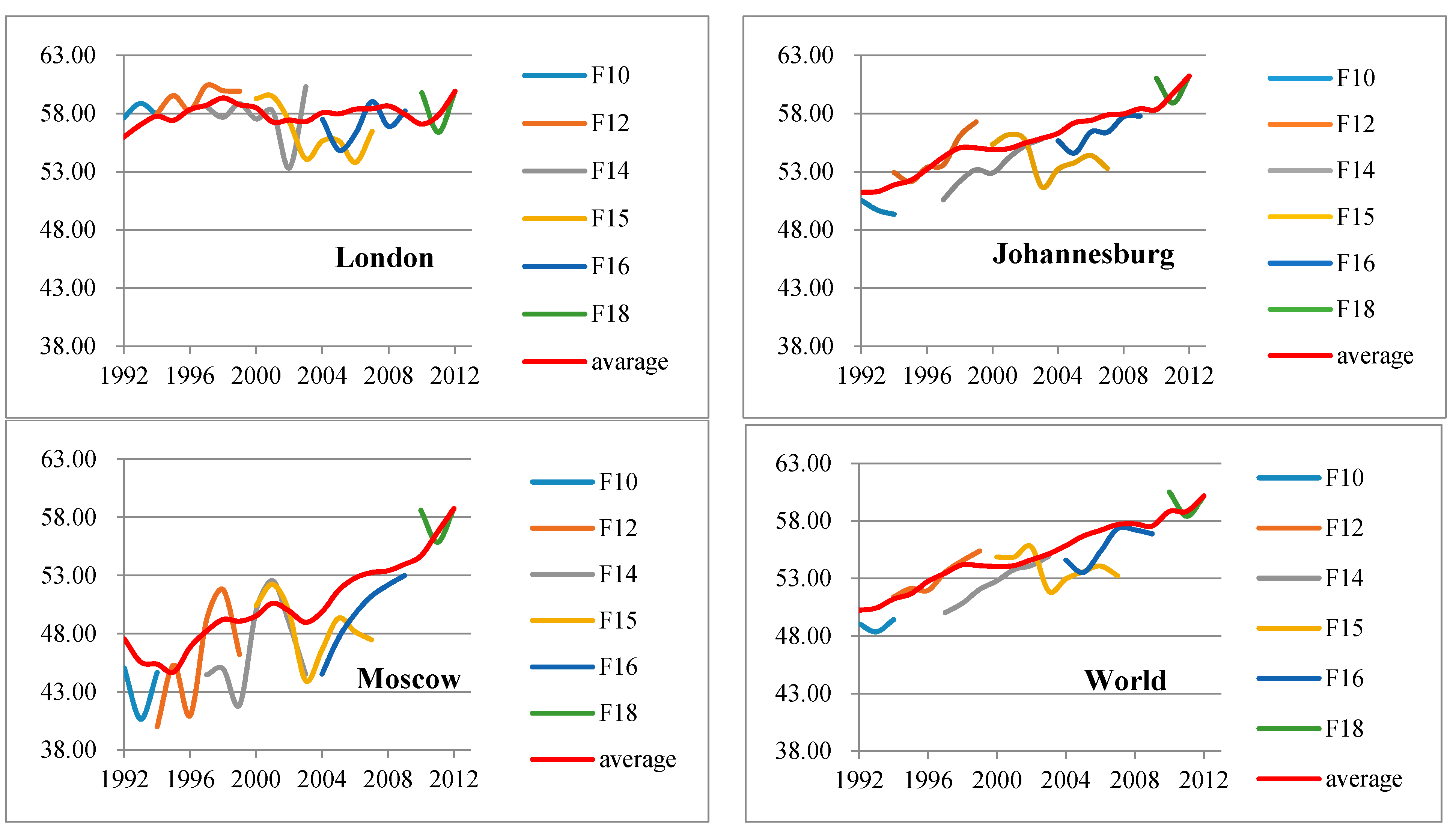
After the intercalibration, intra-annual composition and inter-annual series corrections are common methods used to remove any unstable or inconsistently lit pixels [
30]. Because these pixels may disturb the stability of DN series, we treat them as noisy pixels to be eliminated. We define that the conditional statement DN
n-1 − DN
n ≥ 3 and DN
n+1−DN
n ≥ 3 (n ∈ [1993, 2011]) is probably the noise. There is a low probability that the DN from last year and next year are close, and the intervals between the current year and these before and after years change sharply. This finding is based on the concept of urbanization as a successive process, and the present urbanization stage is related to the past and future. The moving average method is adopted to smooth the series, with three years in succession adopted by an inverted sequence that started from 2011. The noise pixel would be replaced by the mean value of the other DN on the same position in the before and after years. The not-noise pixel would get the mean value of all DN on the same position in these three years. Finally, some examples of the smooth result are shown in
Figure 4. By calibration, the tendency may seem more reasonable than the initial NTL data.
Figure 4.
Examples of DN values of the urbanization area from different satellites after calibration during 1992–2012. F10–F18 express the original DN value, and the “average” line was the final value after calibration.
Figure 4.
Examples of DN values of the urbanization area from different satellites after calibration during 1992–2012. F10–F18 express the original DN value, and the “average” line was the final value after calibration.
3.2. Variation Trend Judgement
We calculated trends on the basis of annual DN and annual maximum NDVI by Theil-Sen slope and used the Mann-Kendall method to test the significance. The Theil-Sen slope estimator is the median of the slopes calculated between observation values at all pairwise time steps [
47]. It is calculated between observations
Xj and
Xi at pairwise time steps
tj and
ti [
48]:
where for NDVI variation,
slope > 0 means restoration and
slope < 0 means degradation.
Similar to the Theil-Sen procedure, the Mann-Kendall test examines the slopes between all pairwise combinations of samples, where each data point is treated as the reference for the data points in successive time periods [
47]. The indicator of Kendall’s
S is defined as [
49]
where
n is the length of the time series, and
xi and
xj are observations at time
i and
j, respectively. When there is independent and identical distribution between data values, then the variance is given by [
50,
51]:
where
σ is the standard deviation. Then the equation for Mann-Kendall significance (
Z) is computed by
where
(equivalent to
p ≤ 0.05) is judged as significant.
6. Conclusions
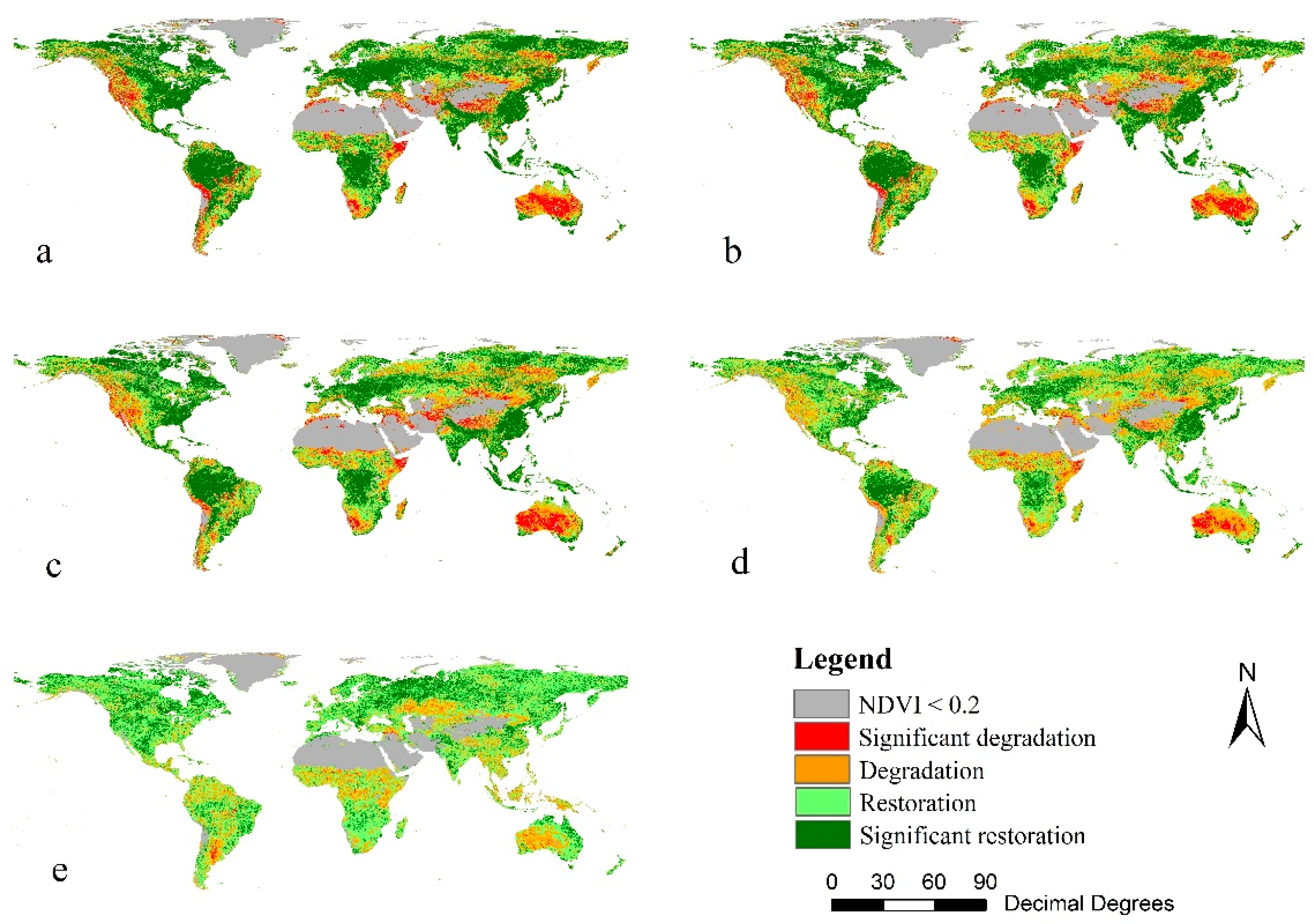
In this study, we have developed a new approach for delineating the different relations between vegetation degradation and urbanization spatially and temporally through the integrative use of NTL data and NDVI data. The result verifies that the urbanization process would not necessarily result in large-scale vegetation degradation. The correlations between urbanization and vegetation variation are diversified in individual cases. Rapid urbanization cities have a high probability of vegetation degradation. However, although cities in Asia experienced the most rapid urbanization, some cities there did not undergo sharp vegetation degradation. Furthermore, with temporal scale variation, the degradation degree varies, which reflects different urbanization stages and climate history. Consequently, we relate the urbanization effect on night light and vegetation to urbanization stage. In the urban expansion stage, the vegetation biomass decrease may be significant. However, when the urbanization turns to an urban aggregation stage, positive demand of urban green space may increase. Therefore, economic growth may not be adopted as an excuse for urban biodiversity loss. By effective urban landscape planning, urban vegetation restoration would replace the degradation, which may contribute to landscape sustainability.
Our approach has a few limitations. First, the spatial resolution of the VIP data set limits the study to focusing on big metropolises rather than small cities. Second, the limitations from coarse resolution and the spillover effect indicate that the accuracy of urbanization information extracted using NTL data requires further improvement [
61,
62,
63]. The new NPP-VIIRS data, which has overcome the relatively low spatial resolution, the lack of onboard calibration and the pixel saturation issue in DMSP/OLS data, is recommended for obtaining higher-quality urbanization information [
64]. Third, the lighting reference area, New York, has been largely stable over time, but that stability does not mean there is no light growth. Fourth, the vegetation variation trend may rely on the NDVI data set, so the trend at the pixel level is, in a sense, uncertain. Nevertheless, the long-term temporal trends of the data set are suitable and unlikely to be replaced by other data sets. The conclusions are credible on the precondition that the result of this article only focuses on the macro scale. Thus, a multi-scale analysis using different data sources will be helpful in reducing uncertainty in future studies.

 ,
, 


