1. Introduction
Although paleontologists and paleoanthropologists use global navigational satellite systems and online data sources such as geological maps to identify potential fossiliferous areas, the process of selecting which areas a field crew should intensively investigate has remained relatively constant for the last century [
1] and there is a certain element of luck in the discovery of new sites. The primary method of locating fossils in the landscape is through intensive and time consuming field surveys in which teams spend large amounts of time traversing the landscape in vehicles and on foot in search of productive areas, which are usually spotted at a distance from a road or higher ground. In an effort to reduce the role of chance, geospatial analytical techniques have recently been used to create predictive models to aid in identifying productive localities.
While the adoption of geospatial techniques in paleoanthropology has been slow as compared to disciplines such as archaeology or geology, some early adopters have incorporated these techniques into their search for hominin fossils. The “Paleoanthropological Inventory of Ethiopia”, a program initiated in 1988 by Ethiopia’s Ministry of Culture and developed by paleoanthropologists Berhane Asfaw and Tim White [
2] mapped the main Ethiopian Rift and Afar Depression using a combination of Landsat Thematic Mapper (TM) satellite imagery, aerial photography, and space shuttle large format camera (LFC) photos to identify geologic features of interest to paleoanthropologists studying early stages of hominin evolution. Aerial photography and satellite images pinpointed locations of interest for ground survey in the Woranso-Mille study area in the central Afar region of Ethiopia [
3]. Njau and Hlusko [
4] used Google Earth supplemented by high resolution IKONOS imagery to locate new paleontological and archaeological sites in Tanzania. Bailey and colleagues [
5] incorporated Landsat 7 Enhanced Thematic Mapper (ETM+) imagery with Shuttle Radar Topographic Mission (SRTM-3) data across southern African landscapes during the Plio-Pleistocene to argue that active volcanism must have played a pivotal role in the habitat choices of early hominins. Nigro and colleagues [
6] used standard surveying techniques to create a 3-D model of the Swartkrans hominin cave site in South Africa and then used GIS methods to plot and analyze the distribution of fossil remains and artifacts in this three-dimensional reconstruction of the cave.
Invertebrate and vertebrate paleontologists have used various geospatial techniques in attempts to reconstruct past environments and to understand the geographic distribution of extinct taxa in the past. In North America, Stucky and colleagues [
7,
8] pioneered the use of satellite imagery to identify vertebrate fossil-bearing rock units of Eocene age in the Wind River Basin of Wyoming. Conroy and colleagues [
9] also used ArcGIS to create Keyhole Markup Language (kml) files for use with Google Earth to record and share results of vertebrate paleontological fieldwork in several sedimentary basins of western North America. Stigall-Rode and colleagues projected locality data for fossil taxa onto a map of the Devonian period in order to model the distribution and habitat ranges of extinct taxa [
10,
11]. Another interesting application of geospatial techniques in paleontology [
12] used a GIS to analyze the utility of biostratigraphic dating methods applied to vertebrate faunal and floral assemblages during the Triassic of North America and Europe. Ghaffar [
13] created digital contour maps of the Dhok Bun Ameer Khatoon site in the Siwalik Hills of Pakistan and used these models to explore the fossil distribution of the Miocene giraffid
Giraffokeryx punjabiensis.
Many of the works previously discussed relied upon visual inspection of remotely sensed imagery to guide ground surveys in search of fossil vertebrates, hominins, or archaeological sites. Although archaeologists have been developing and testing predictive site location models for several decades [
14,
15,
16], predictive modeling has been rarely utilized by paleontologists or paleoanthropologists. Oheim [
17] developed a model to predict the location of dinosaur fossils in the late Cretaceous Two Medicine Formation of north-central Montana. She performed a suitability analysis, an approach commonly used by archaeologists, which incorporates several types of data into a GIS, including geologic maps, land cover maps, road networks, and elevation. This analysis resulted in a raster data layer in which each grid cell had a value based on environmental suitability that predicted the likelihood of locating fossils at that location. This model was field tested by systematically surveying areas of both high and low probability. The number of fossils found per square kilometer was used to create a fossil density map that was highly correlated with the predicted score. Chew and Oheim [
18] used GIS analyses to explore biases in the fossil mammal record from the earliest Eocene of the Bighorn Basin in Wyoming. Their results suggested that sampling area (calculated within their GIS by digitizing fossil localities from topographic maps) added significant bias to calculations of species richness both at the level of individual localities and across the entire basin.
Another geospatial method of predicting where fossils can be found is by classifying imagery. Malakhov and colleagues [
19] used a spectral angle mapping technique to classify Landsat ETM+ imagery of fossiliferous strata in southern Kazakhstan. Conroy used an unsupervised classification approach [
20] and Conroy and colleagues [
21] classified Landsat ETM+ imagery using a maximum likelihood approach in the Uinta Basin of Utah. In the Great Divide Basin in Wyoming, two of the authors of this paper used an Artificial Neural Network (ANN)-based technique to classify Landsat ETM+ imagery with the goal of identifying new localities [
22,
23]. By training the ANN to recognize the spectral signatures of known fossil localities, they created a classified image that included predicted localities throughout the basin. It was found that the medium resolution Landsat imagery was adequate for a general reconnaissance of the 10,000 km
2 basin, but problems with over prediction led to frequent false positive indications. In an attempt to improve on these results, this paper explores an object-oriented approach in which higher resolution imagery of areas of interest are analyzed in greater detail. The ANN-based Landsat ETM+ model is also used to compare the object-based models that are the subject of this paper.
2. Study Area
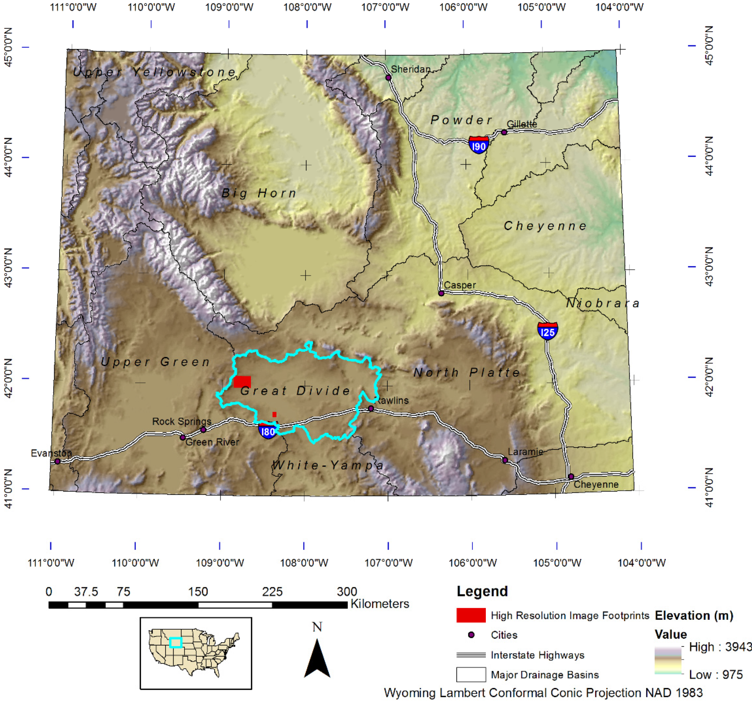
Located in southwestern Wyoming USA (see
Figure 1), the Great Divide Basin (GDB) is an internal drainage basin that forms the northeastern part of the Greater Green River basin. The basin is encircled by the Continental Divide, which splits at South Pass and rejoins near Rawlins, WY. The GDB is bounded by the Wamsutter Arch in the south, the Rock Springs Uplift to the west, the eastern portion of the Wind River Mountains and the Sweetwater Arch to the north, and the Rawlins Uplift to the east. Interstate highway 80 parallels the Wamsutter Arch along the southern edge of the GDB between the cities of Rawlins in the east and Rock Springs in the west.
Many geological surveys of the GDB are mainly concerned with understanding and mapping its copious hydrocarbon and mineral resources [
24,
25,
26,
27,
28], while paleontological efforts prior to our research team’s work over the past twenty years were minimal [
29,
30]. This region of Wyoming is drastically different today than it was during the Eocene epoch (56–38 million years ago), when the climate was tropical and therefore significantly warmer and wetter than today. Throughout the Eocene, the Greater Green River Basin was the site of a large freshwater lake known to geologists as Lake Gosiute. The lake expanded and contracted multiple times throughout the Eocene due to climate change and tectonic activity [
31], resulting in a complex inter-tonguing geological layer cake of fluvial and lacustrine sediments. At various times throughout the Eocene, Lake Gosiute encompassed the entire Greater Green River Basin (including parts of modern day Wyoming, Utah and Colorado), while at other times it was separated into multiple, smaller lakes. The Fort Union and Wasatch formations are fluvial units that outcrop throughout the Greater Green River Basin. These are the beds of most interest to this research since they often contain remains of terrestrial vertebrates who lived, died, and were fossilized along the rivers, streams and deltas of late Paleocene to early Eocene southwestern Wyoming. Green River Formation deposits are lacustrine in origin, representing the sediments created by Lake Gosiute itself, and they contain abundant fish fossils [
32].
Figure 1.
The Great Divide Basin in southwestern Wyoming (highlighted in blue).
Figure 1.
The Great Divide Basin in southwestern Wyoming (highlighted in blue).
While vertebrate fossils spanning the late Paleocene through the late Eocene epochs can be found in the GDB, our research team focuses on the mammals and other vertebrates that lived during the earliest part of the Eocene, the so-called Wasatchian North American Land Mammal Age (NALMA) [
33]. The transition from the Paleocene to the Eocene epochs, which occurred approximately 56 million years ago (MYA) was a critically important moment in the history of life on Earth [
34,
35,
36,
37], marked by a massive perturbation in the Earth’s carbon cycle caused by an enormous release of methane into the atmosphere from oceanic clathrate deposits [
38,
39]. The resulting greenhouse warming led to an estimated 5–8 degree Celsius rise in global temperatures that lasted for several tens of thousands of years and resulted in an enormous faunal and floral turnover on land and in the oceans [
39]. This event has come to be known as the Paleocene Eocene Thermal Maximum (PETM), and it was accompanied by the extinction of many typical Paleocene taxa and the origination (and spread across the northern continents) of a modern mammalian fauna marked by the first appearance of primates, artiodactyls and perissodactyls [
35].
Vertebrate fossils in the GDB are typically preserved in the fluvial channel sandstones and overbank deposits of the Wasatch Formation. The fossils of terrestrial animals are usually isolated teeth, jaws, and postcranial bones that have been transported by stream action. Whole or partial skeletons, skulls, or articulated bones are extremely rare. In addition to mammals such as early primates, rodents, hooved animals and carnivores, the remains of turtles, crocodiles, lizards and fish are frequently found. As the fossils erode out of the sandstones due to the action of wind and water, they are deposited in the loose sands found at the base of sandstone outcrops. Some fossils are found in situ within the sandstone matrix and can be carefully removed from the surrounding rock using dental picks. Dry or wet screening is often incorporated in the search for small fossils such as teeth. Exposed silt and mudstone areas also sometimes contain isolated small fossils.
Over a 22-year period, the authors have identified 125 productive localities in the Great Divide Basin using the traditional search technique in which geological and topological maps are consulted to identify potentially productive areas that are accessible and have the correct fluvial geology. Field crews of five to fifteen workers traverse the landscape in vehicles or on foot and visually identify sandstone outcrops and barren areas that undergo a search that typically takes upwards of an hour, depending on the size and complexity of the site. The area of these 125 localities is approximately 1.75 km2, a tiny fraction of the 10,000 km2 basin. In a typical month-long field season, approximately six new localities are found, with most of these being clustered near the sparse road network in the GDB.
A major limitation of the traditional search methodology is the dependence on the available geological maps, which are often highly generalized and, in some cases, poorly represent the complex fluvial and lacustrine sedimentary surficial geology. This was found to be the case while surveying in areas mapped as the Niland tongue of the Wasatch formation. In some cases, the sedimentary deposits and fossils found here were more indicative of a lacustrine depositional environment, indicating the local geology was most likely part of the Tipton tongue of the Green River formation. A second aspect of inaccuracies in geologic maps is the fact that WMU-VP-222 (
Figure 2), an Eocene sandstone outcrop (Wasatch Fm.) is mapped as Quaternary sand. This probably is a result of this relatively small outcrop being below the minimum mapping unit of the available geological map.
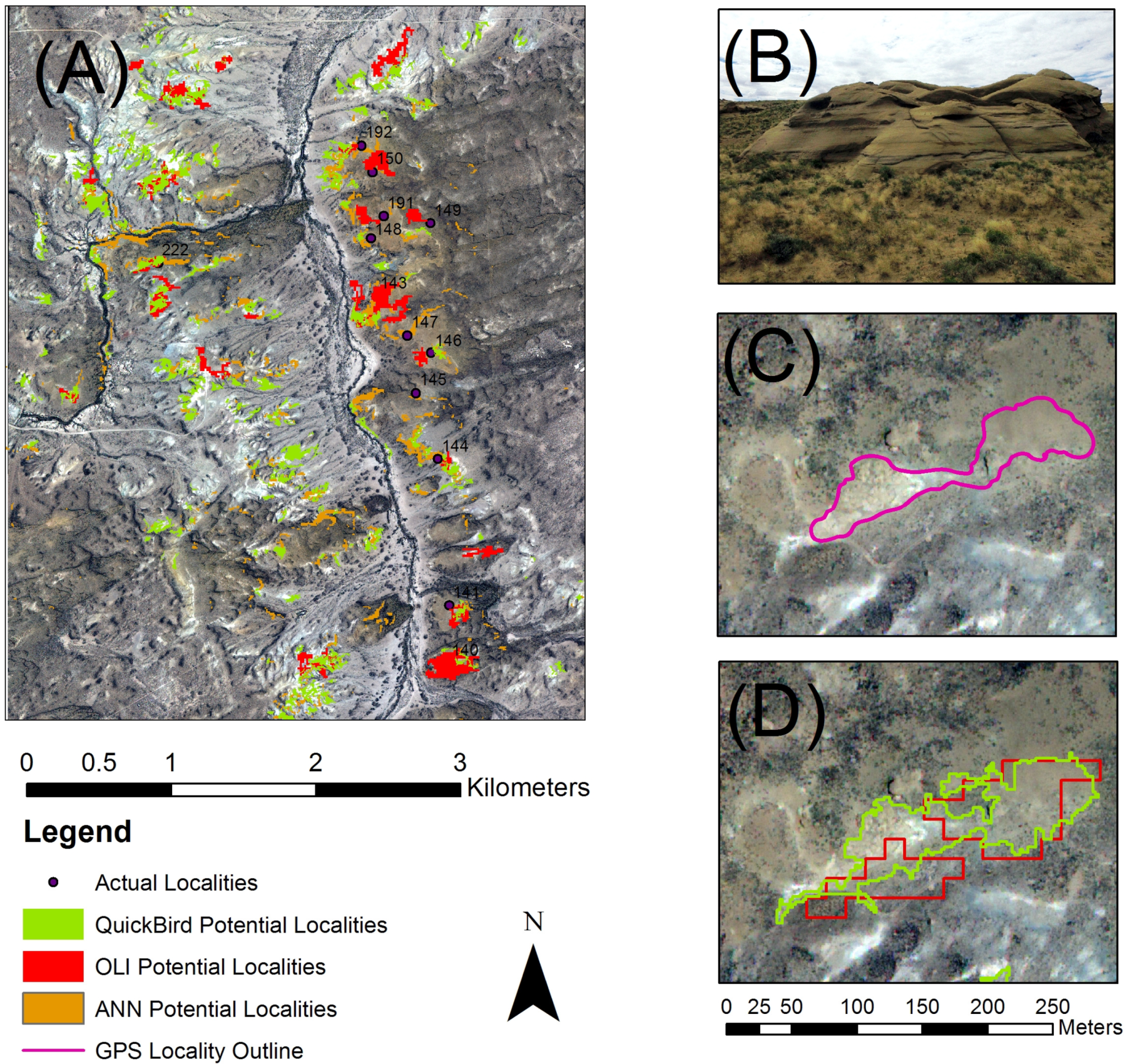
Figure 2.
QuickBird image of the training area (A) showing ANN-, OLI-, and QuickBird-based model results and productive localities discovered in previous field seasons; (B) Ground level view of a sandstone outcrop at an example locality. The outer edge of the whole locality measured with a GPS (C); (D) The highlighted image objects for the QuickBird model (green) and the Landsat 8 OLI model (red). Because these localities are on public land and are therefore subject to possible illegal looting, the exact coordinates cannot be publicized under the terms of our collection permit.
3. Data and Methodology
This research explores the use of imagery with higher spatial resolution than was used in previous work in an effort to more accurately delineate the localities and reduce the problem of over prediction. Since high spatial resolution sensors represent objects of the size of typical fossil localities (approximately 5000 to 20,000 m2 in this area) with many more pixels than would be the case in medium resolution imagery, data volume and economic constraints limited analysis to selected small patches where surface features are represented by groups of pixels.
Geographic object-based image analysis (GEOBIA) is a term coined by Hay and Castilla [
40] to differentiate techniques that analyze groups of homogeneous pixels (image objects) from raster analyses that operate on a per-pixel basis. Multi-pixel image objects allow more complex analyses based on statistics, shape parameters and contextual relationships [
41] and GEOBIA techniques can reduce mis-registration and shadowing effects [
42]. The most important advantage is the fact that the image objects created can directly correspond to a real world object [
43], such as a known highly productive fossil locality. Blaschke
et al. [
44] argue that GEOBIA has evolved sufficiently to be designated a new scientific paradigm with specific tools, software, methods, rules and language.
The 2013 field season used high resolution QuickBird satellite imagery of the Freighter Gap to Pinnacles area, a section in the northwest part of the Great Divide Basin that was deemed high priority for exploration by previous research [
22]. A 160 km
2 QuickBird image from 9 September 2009 was selected for the analysis, while a 25 km
2 image of an area in the southern part of the GDB was acquired as a training site for the feature extraction model. Both of these images were pan sharpened to a spatial resolution of 0.6 m using the Gram-Schmidt module in module in ENVI™ version 5.1.
Figure 1 shows the image footprints in red and
Figure 2A shows the training site area. The 25 km
2 image has several localities that were identified in earlier surveys, including WMU-VP-222, the most productive locality that has been identified to date within the GDB (
Figure 2). It was discovered in 2002 and has provided thousands of mammalian fossils, including important adapid and omomyid primate species. For the 2014 field season, a Landsat 8 Operational Land Imager (OLI) image from 27 June 2013 was used to extend the predictive model to other parts of the basin. Multispectral bands 2 through 7, which include the visible, near-infrared and two shortwave infrared bands were used, and the coastal (band 1) and cirrus (9) bands were excluded. This image was also pan-sharpened to a spatial resolution of 15 m using the panchromatic band (band 8).
Other data included a digital elevation model (DEM), a surficial geology map, a map of Wyoming roads, and the watershed boundaries of the Greater Green River basin. The DEM has a ten meter resolution and was developed from the National Elevation Dataset. The geologic map was created by the Wyoming State Geological Survey in 1998 at a 1:500,000 scale.
The results of an earlier Artificial Neural Network (ANN) per-pixel classification of a Landsat 7 Enhanced Thematic Mapper + (ETM+) image obtained on 8 August 2002 were used to compare the GEOBIA results to a more traditional analysis. The ANN classification process (detailed in [
22,
23]), divided the basin into five land cover classes: barren, forest, scrubland, wetland and localities. The map of the pixels classified as localities was used as a basis for comparison and is displayed in
Figure 2,
Figure 3 and
Figure 4 using orange symbology.
For the GEOBIA analysis, a “divide and conquer” exclusionary classification scheme was adopted. Areas of the image were classified into crisp classes using Boolean descriptors based on the above parameters and then excluded in a stepwise manner until only the suitable areas of the image remained. A series of classes was generated including: flatland, sloped land, vegetation, roads, cloud, and finally potential localities. The multiresolution segmentation algorithm in the eCognition Developer 64™ software package was used to segment the imagery into image objects. The 25 km
2 high resolution image was used to develop the rule set for the segmentation and feature extraction of the Freighter Gap-Pinnacles image (
Table 1). The multi-resolution segmentation algorithm was used and the segmentation parameters were developed using a heuristic process to determine the appropriate values. This process is hierarchical and iterative as each segmentation operates on previous segmentations, creating image objects that nest within larger super-objects, and resulting in a multi-scale segmentation of the image. A total of four nested hierarchical levels of segmentation were performed, with scale parameters (roughly analogous to the size of image objects) of 100, 50, 25 and 10. The compactness variable was set to 0.5 and the shape parameter was set to 0.1. Because localities can range from long, narrow outcrops along a ridge to compact, isolated forms, shape was only marginally incorporated in the segmentation and both the smoothness and compactness aspects of shape were equally balanced.
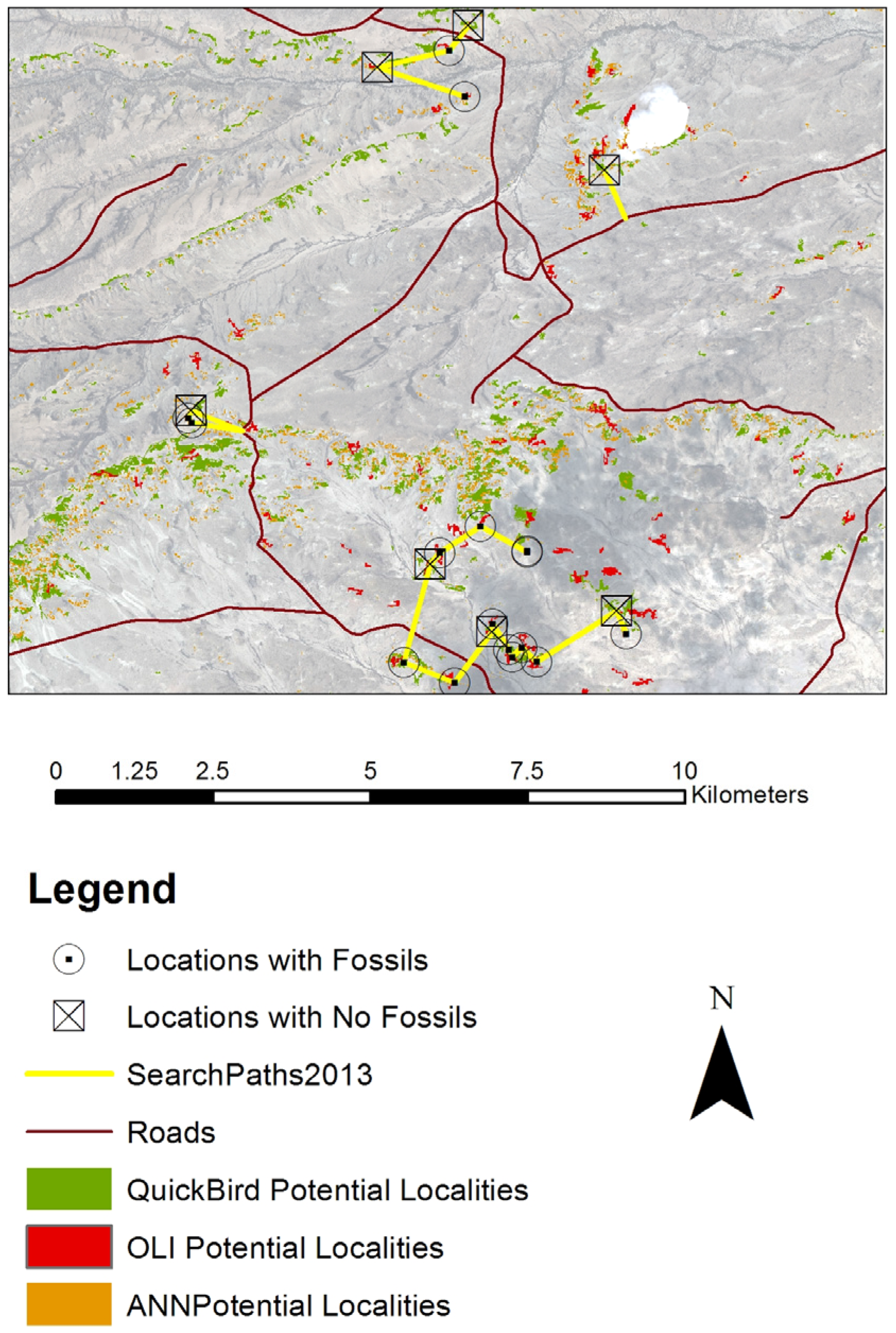
Figure 3.
Freighter Gap/Pinnacles QuickBird image showing potentially fossiliferous ANN-, OLI-, and QuickBird-based image objects and selected high priority candidate localities.
Figure 3.
Freighter Gap/Pinnacles QuickBird image showing potentially fossiliferous ANN-, OLI-, and QuickBird-based image objects and selected high priority candidate localities.
Once each multi-resolution segmentation was completed, spectral difference segmentation was performed for each level. Each segmentation created a large number of individual image objects, often with neighboring image objects that were spectrally similar. The spectral difference segmentation algorithm merged neighboring image objects according to their mean image layer intensity values. Neighboring image objects were merged if the difference between their layer mean intensities was below the value given by the maximum spectral difference value. A maximum spectral difference value of 10 was chosen to reduce the total number of image objects and decrease total computation times.
The goal of the segmentation was to create an image object that matched WMU-VP-222, a productive fossil locality in the 25 km2 image. The level three and four segmentations (scale parameters of 25 and 10 for the QuickBird imagery, or a scale parameter of 50 in the case of the Landsat 8 OLI image, best delimited the areal extent of the locality as measured by GPS in previous field seasons. The segmented image was then analyzed to develop the classification rule set. Statistical values such as mean brightness of the image objects that corresponded with WMU-VP-222 were used to determine the parameters for the feature extraction.
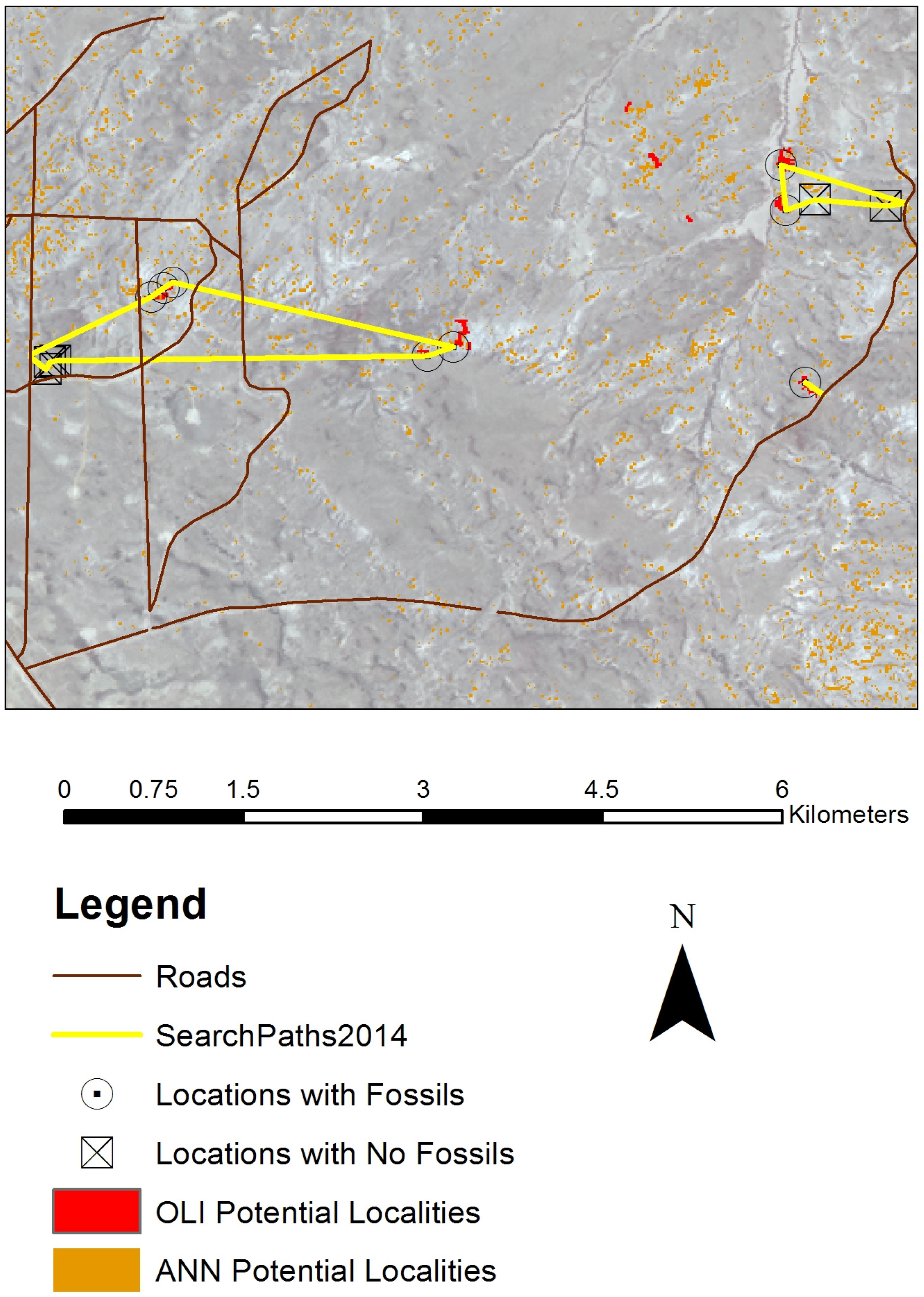
Figure 4.
Landsat 8 OLI image of the 2014 search area southeast of Dugout Draw showing image objects from OLI-based and ANN-based models and results of field searches of selected high priority sites.
Figure 4.
Landsat 8 OLI image of the 2014 search area southeast of Dugout Draw showing image objects from OLI-based and ANN-based models and results of field searches of selected high priority sites.
Table 1.
eCognition rule set for the QuickBird imagery.
Table 1.
eCognition rule set for the QuickBird imagery.
| Segmentation | | |
|---|
| | Multiresolution | |
| | | 100 (shape:0.1 compct:0.5) creating “Level 1” |
| | | At Level 1: spectral difference 10 |
| | | 50 (shape:0.1 compct:0.5) creating “Level 2” |
| | | At Level 2: spectral difference 10 |
| | | 25 (shape:0.1 compct:0.5) creating “Level 3” |
| | | At Level 3: spectral difference 10 |
| | | 10 (shape:0.1 compct:0.5) creating “Level 4” |
| | | At Level 4: spectral difference 10 |
| Classification | | |
| | Level 3 | |
| | | Unclassified with Mean Slope Layer 8 ≥ 6 at Level 3: SlopedLand |
| | | Unclassified with Mean Slope Layer 8 < 6 at Level 3: FlatLand |
| | | SlopedLand with NDVI ≥ 0.16 at Level 3: Vegetated |
| | | FlatLand and SlopedLand with Length/Width (geometry ratio) > 4 at Level 3: Road |
| | | SlopedLand with Brightness ≥390 at Level 4: Locality |
| | Level 4 | |
| | | Unclassified with Mean Slope Layer 8 ≥ 6 at Level 4: SlopedLand |
| | | Unclassified with Mean Slope Layer 8 < 6 at Level 4: FlatLand |
| | | SlopedLand with NDVI ≥ 0.16 at Level 4: Vegetated |
| | | FlatLand and SlopedLand with Length/Width (geometry ratio) > 4 at Level 4: Road |
| | | SlopedLand with Brightness ≥ 390 at Level 4: Locality |
Once the specific parameters for the multi-resolution segmentation were determined using the 25 km
2 image, the segmentation was applied to the Freighter Gap/Pinnacles image. Slope is an important landscape characteristic for extracting potential localities. The most productive localities in the GDB are located along cliff faces, where a more resistant cap of sandstone or limestone overlies less resistant fossil-bearing sediments [
22]. Flat areas were excluded based on the mean slope values of the image objects calculated from the slope layer. A value of six percent slope was chosen as the threshold based on the distribution of slope values measured at the localities that were discovered in earlier field seasons. All areas with six percent mean slope or higher were classified as high slope and all below six percent were classified as low slope. The areas of low slope were then excluded from consideration. The primary vegetation in the GDB is sagebrush, mixed grass, and saltbrush, and fossils are typically not found in heavily vegetated areas. These areas were excluded using the mean Normalized Difference Vegetation Index (NDVI) values for each image object. An NDVI threshold of 0.16 was adopted with image objects at or above this value corresponding to areas with sagebrush or riparian vegetation. A variety of values were tested and visually inspected to determine if large patches of sagebrush were adequately classified.
Since fossils are typically found in surface scatters, any human activity, such as grading, paving, or frequent travel, will accelerate the decomposition of fossils. Therefore, areas of human disruption of the landscape are not generally good locations for prospecting for fossils. While most roads in the GDB are simple two-track trails, some roads have been graded or paved by the county road department or oil and gas companies in the region. The pads surrounding the increasing number of oil and gas wells scattered throughout the basin are also not good candidate areas, but these are large and flat enough to be included in the low slope class. A road class was derived using the length/width ratios. A high brightness value reflected the fact that the bare soil of the dirt roads in the images was significantly brighter than their surroundings. The length/width ratios identified the image objects that were thin in shape. Roads were excluded to limit potential localities to undisturbed areas.
In the Freighter Gap/Pinnacles QuickBird image, a small patch of cloud cover in the northeastern portion of the image was manually outlined and excluded. After excluding flatlands, vegetated areas, clouds, and roads, the remaining image objects with a mean brightness value of less than or equal to 390 were excluded. In the shadowed area relating to the cloud, the rule set was re-run with the brightness value for this last step lowered to 222. Any image object remaining in the high slope classification that met this mean brightness parameter was then classified as being a potentially fossiliferous location.
A similar rule set was applied to the pan-sharpened Landsat 8 OLI image of the entire Great Divide Basin. In this case only two levels of segmentation, with scale parameters of 100 and 50 were performed, as smaller scale parameter values yielded objects consisting of only a few pixels. The threshold brightness value for identifying potential localities was 17,500. No clouds were present, so brightness adjustments for shadow areas were not necessary. A completely segmented and classified image was now completed.
Figure 2A shows the results of the extraction of potential localities, with a ground level photograph of an example outcrop (
Figure 2B), a larger scale image that shows the outline of the whole locality as measured by GPS (
Figure 2C), and the model output for this area (
Figure 2D) with the QuickBird image objects outlined in green and the Landsat 8 OLI objects in red.
The models were verified using twelve known fossil localities to the east of WMU-VP-222 in the 25 km
2 image that were found in earlier field seasons using the traditional search technique (
Figure 2A). In the case of the QuickBird-based model, eleven of the twelve localities were within 100 m of an image object. Reducing the brightness threshold below 390 resulted in a large increase of highlighted objects. The Landsat 8 OLI model highlighted the same eleven localities. Ten of the 12 fossil localities corresponded to pixels highlighted by the ANN classification.
The final classified image objects were then exported from the eCognition software as an ArcGIS feature class. Only the image objects classified as potential localities were exported for all four levels of segmentation. The surface geology map was added to these maps and any classified image objects that did not fall within the Wasatch formation were excluded. This was the final step in the classification process and resulted in polygons that indicate areas of the image that met all criteria for being potentially fossiliferous. A map of the road network of the basin was added to each map to provide guidance to accessing high priority sites.
The predictions that were derived from the QuickBird image of the Freighter Gap/Pinnacles area were tested during the July 2013 field season. The maps of the extracted image objects indicated locations within the satellite images that met the criteria for containing fossils. However, there were many individual predicted image objects in the image and it was impossible to survey each potential locality in the limited time allotted. In order to further refine the areas to be surveyed, 17 high priority survey points were selected from the Freighter Gap/Pinnacles image along four paths followed by the field crew (
Figure 3).
The maps of image objects corresponding to potentially productive localities were exported into ArcPad and then loaded onto a Topcon GRS-1 GPS receiver. These ArcPad maps included the four classified segmentation levels, a road map, surficial geology map, the satellite image, a point feature of known fossil localities, and finally a point feature of the selected survey points. The GPS receiver was then used in the field to navigate to selected survey points. Nine potential localities that were not predicted by the model were also searched by the field crew as it transited between the survey points. These sites were generally unvegetated mudstone areas and flat areas of exposed sandstone that would normally be searched if they were spotted in a traditional survey. The unpredicted sites serve as “negative” localities, so that the reported statistics evaluate the model’s ability to distinguish productive fossil localities from “searchable” sites. Because the sampling frame consists of potential localities, rather than random locations, the sampling scheme is conservatively biased. The limited number of sites that were searched was dictated by the difficult logistics of transporting a field survey crew and the fact that meaningful searches of a single candidate site can take upwards of an hour. A sampling scheme based on complete spatial randomness would necessarily involve searching a large number of locations such as sagebrush flats and sand dunes that would not normally be searched. Any localities that were searched in the field were recorded in the map with a new, sequentially numbered point feature that included information such as: coordinates, date, and brief descriptions of the types of fossils recovered and of the local geology.
4. Results and Discussion
A total of 26 sites were searched for fossils in 2013 as shown in the confusion matrix (
Table 2), 18 of which had fossils and eight that did not. The eight negative sites were sandstone outcrops or mudstone areas that were searched for fossils as they were encountered in the field when transiting to or between the 17 sites that were highlighted by the predictive model. In the model based on the QuickBird image, 14 sites were within a 100 m buffer of a predicted high priority survey point, and five of the negative sites were not associated with image objects. This yielded a 73.1 percent correct classification rate. Cohen’s Kappa statistic was 0.389, indicating the model showed an approximately 39 percent improvement over random chance [
45,
46]. The user’s accuracy is the probability that an object predicted to either contain fossils or not is correctly identified so that it represents a measure of errors of commission. Producer’s accuracy represents the probability that a locality that actually contains or does not contain fossils is correctly highlighted by the model and represents a measure of errors of omission. The user’s and producer’s accuracies for the predicted fossil localities were approximately 0.80, indicating relatively low errors of commission and omission. However the lower user’s accuracy (0.56) for the localities that were searched but not predicted by the model indicates that the model was not as effective at identifying areas that are not likely to contain fossils.
Table 2.
Results of 2013 field season from the Freighter Gap/Pinnacles QuickBird image.
Table 2.
Results of 2013 field season from the Freighter Gap/Pinnacles QuickBird image.
| Prediction | Ground Truth | |
|---|
| | Fossils Present | Fossils Absent | User’s Accuracy |
| Fossils Present | 14 | 3 | 0.82 |
| Fossils Absent | 4 | 5 | 0.56 |
| Producer’s Accuracy | 0.78 | 0.63 | |
| Percent Correct | 73.1% | Cohen’s Kappa 0.389 | |
When the basin-wide model derived from the Landsat 8 OLI image was developed prior to the 2014 field season, the predictions were applied retrospectively to the 2013 field results from the Freighter Gap to Pinnacles area.
Table 3 is a confusion matrix for this retrospective analysis and
Figure 3 also shows the model results. The OLI-based model was more conservative with fewer potentially productive localities predicted in the Freighter Gap-Pinnacles area. This is reflected in the lower correct classification rate (65.4%) with only 11 of the 18 fossiliferous localities being correctly identified. The number of false positives was reduced to two, and Cohen’s Kappa was reduced to 0.308. While the user’s accuracy (0.85) was a bit higher than the QuickBird-based model due to the lower number of false positives, the lower producer’s accuracy (0.61) indicates that false negative indications missed seven productive localities. The Landsat 8 OLI GEOBIA model was overly conservative as evidenced by the low user’s accuracy (0.46) for the fossils absent prediction. Adjusting the threshold brightness value for identifying potential localities to a value lower than 17,500 would highlight more localities as potentially productive and would likely improve these results.
Table 3.
Retrospective results of 2013 field season from the Landsat 8 OLI image.
Table 3.
Retrospective results of 2013 field season from the Landsat 8 OLI image.
| Prediction | Ground Truth | |
|---|
| | Fossils Present | Fossils Absent | User’s Accuracy |
| Fossils Present | 11 | 2 | 0.85 |
| Fossils Absent | 7 | 6 | 0.46 |
| Producer’s Accuracy | 0.61 | 0.75 | |
| Percent Correct | 65.4% | Cohen’s Kappa 0.308 | |
Table 4 contains the results from the Landsat 7 ETM+ ANN-based model applied retrospectively to the 2013 localities. This model was less conservative than either of the GEOBIA models and highlighted more areas as potentially productive. The lower Cohen’s Kappa (0.224) is a reflection of this overprediction and the lack of specificity in areas predicted to not be fossiliferous resulted in low user’s and producer’s accuracies (0.50 and 0.63, respectively).
Table 4.
Retrospective results of 2013 field season from the Landsat 7 ANN-based predictive model.
Table 4.
Retrospective results of 2013 field season from the Landsat 7 ANN-based predictive model.
| Prediction | Ground Truth | |
|---|
| | Fossils Present | Fossils Absent | User’s Accuracy |
| Fossils Present | 15 | 5 | 0.75 |
| Fossils Absent | 3 | 3 | 0.50 |
| Producer’s Accuracy | 0.83 | 0.63 | |
| Percent Correct | 69.2% | Cohen’s Kappa 0.224 | |
In the 2014 field season, image objects derived from the Landsat 8 OLI image were used to direct the field crew to seven potential localities southeast of Dugout Draw, a previously unsurveyed portion of the GDB (
Figure 4). Seven additional sites that were not predicted by the model were searched as well. In the confusion matrix (
Table 5), six of the nine localities that contained fossils were successfully predicted and four of the five negative sites did not have a predicted image object at that location. This yielded a 71.4 percent correct classification rate with a Cohen’s Kappa statistic of 0.429. The overly conservative nature of this model is evident in the relatively low user’s accuracy for the fossils absent prediction (0.57) and the low producer’s accuracy (0.67) for the sites that actually contained fossils.
The tendency for the ANN-based model to over predict sites with fossils present is evident in the retrospective results for 2014 (
Table 6). The user’s accuracy for the fossils present prediction is the lowest of any of the comparisons here, and the model overpredicts to the extent that three of the five sites with no fossils were highlighted, resulting in a producer’s accuracy of only 0.40.
Table 5.
Results of 2014 field season from the Dugout Draw area using the Landsat 8 OLI image.
Table 5.
Results of 2014 field season from the Dugout Draw area using the Landsat 8 OLI image.
| Prediction | Ground Truth | |
|---|
| | Fossils Present | Fossils Absent | User’s Accuracy |
| Fossils Present | 6 | 1 | 0.86 |
| Fossils Absent | 3 | 4 | 0.57 |
| Producer’s Accuracy | 0.67 | 0.80 | |
| Percent Correct | 71.4% | Cohen’s Kappa 0.429 | |
Table 6.
Results of 2014 field season from the Dugout Draw area using the Landsat 7 ANN-based predictive model.
Table 6.
Results of 2014 field season from the Dugout Draw area using the Landsat 7 ANN-based predictive model.
| Prediction | Ground Truth | |
|---|
| | Fossils Present | Fossils Absent | User’s Accuracy |
| Fossils Present | 8 | 3 | 0.72 |
| Fossils Absent | 1 | 2 | 0.67 |
| Producer’s Accuracy | 0.89 | 0.40 | |
| Percent Correct | 71.4% | Cohen’s Kappa 0.317 | |
5. Conclusions
The primary goal of the survey work performed in the Great Divide Basin was the recovery of Eocene vertebrate fossils. Of particular interest were mammalian fossils, specifically primates (such as adapids and omomyids). Over the past twenty years of fieldwork in this area, it has been recognized that sandstone outcrops and barren areas of mud or siltstone are the most likely locations to contain mammalian and primate fossils [
22]. The goal of both of these predictive models is to recognize these potentially fossiliferous locations remotely and pinpoint them within the landscape. Survey teams can then be guided to previously unsurveyed locations or areas that possibly have been overlooked during previous field seasons. The overall success rate of these models, approximately 65% to 73%, with Kappa values from 0.3 to 0.4, is a moderate success and does improve on the traditional search method of spotting potential localities from roads or on foot.
Previous methods of survey relied on visual inspection of topographic and geologic maps to locate areas of interest. The survey team would then travel to these areas and physically search for visible sandstone outcrops, which were relatively close to and generally visible from roads. By using methods such as those proposed here, survey teams can use GPS to navigate to potentially productive locations that are not visible from the road network. This expands the search area significantly in areas such as the GDB that have sparse road networks, meaning that field crews can utilize their time more efficiently.
There are some issues that have come to light in the execution of this research. The first of these is that the scale parameter for the multiresolution segmentations and the spectral difference thresholds were heuristically determined, thus limiting the transferability of these models to other imagery sources, dates, and areas. This is an inherent problem in any expert system, although in the case of GEOBIA, research into statistical methods such as the Estimation of Scale Parameter [
47] that minimize within object local variance while maximizing between object variance provide some guidance in this regard. Other parameter optimization techniques [
48,
49,
50] have been recently introduced and the ESP technique was automated and updated to include multidimensional data [
51], and these would likely improve the segmentation process and may obviate the need for using the spectral difference merging of size-limited image object that otherwise have similar characteristic features to neighboring objects.
Using the mean brightness of the image objects to classify the sandstone outcrops is a rather simplistic method that does not take full advantage of the spectral signature of the localities. The result is that there were quite a few “false positives” in the classification. Some of the areas that were highlighted by the models were found to consist primarily of claystones and mudstone, as opposed to sandstones, and although these have contained isolated fossils in some cases, the probability of finding fossils in these areas is low. A more narrowly specified spectral analysis that focuses exclusively on sandstone outcrops could possibly be more successful. Previous work [
20,
21,
22,
23] has shown some promise in this regard on a per-pixel basis, but differentiating the spectral signatures of sandstone outcrops from the surrounding eroded and windblown sand and separating the fluvial Wasatch formation from the lacustrine Green River formation are problems that remain elusive.
The slope mask could have benefited from a higher resolution DEM that would more closely match the spatial resolution of the QuickBird imagery. Details of some of the smaller localities were inevitably lost in the relatively coarse 10 m mesh. The models would have been more efficient and flexible if the geological data were incorporated as a thematic layer in the rule set rather than using this map as a post hoc mask.
Another improvement that could be incorporated is a more robust ground truthing of the resulting classification. In this research, areas searched were those classified as being potentially fossiliferous by the models or those areas encountered in the field that looked promising but were not predicted. This particularly limited the number of negative sites that were searched, so that the proportion of fossiliferous sites did not reflect their extreme rarity in the total landscape. In 22 years of searching for localities in the GDB using traditional techniques, the authors have identified 125 known productive localities in approximately 20 actual months of fieldwork with prospecting crews typically ranging from five to fifteen workers). The search paths in the 2013 and 2014 field seasons did not encounter enough negative sites along the search paths to achieve this proportion so that the unbalanced survey design skewed the kappa statistic downward [
45].
In spite of these limitations, this research has shown that the GEOBIA methodology of analyzing high resolution imagery has the potential to improve paleontological and paleoanthropological field surveys, and in this example, it outperforms the per-pixel ANN-based model using medium resolution imagery. A total of 27 new productive fossil localities were identified in the 2013 and 2014 field seasons, 20 of which were highlighted by the QuickBird or Landsat 8 models. The methodology developed here is a fairly simple segmentation and classification scheme that was shown to have moderate success in locating fossils in the field. With further refinement of this methodology, more accurate predictive models can be developed and the success rate of fossil recovery can be greatly increased. This will result in a saving of time and money while performing fieldwork and will ultimately lead to the recovery of more fossils, and a greater understanding of life in the past.


