
Predicting Grapevine Water Status Based on Hyperspectral Reflectance Vegetation Indices

 ,
,
Abstract
:
1. Introduction
2. Material and Methods
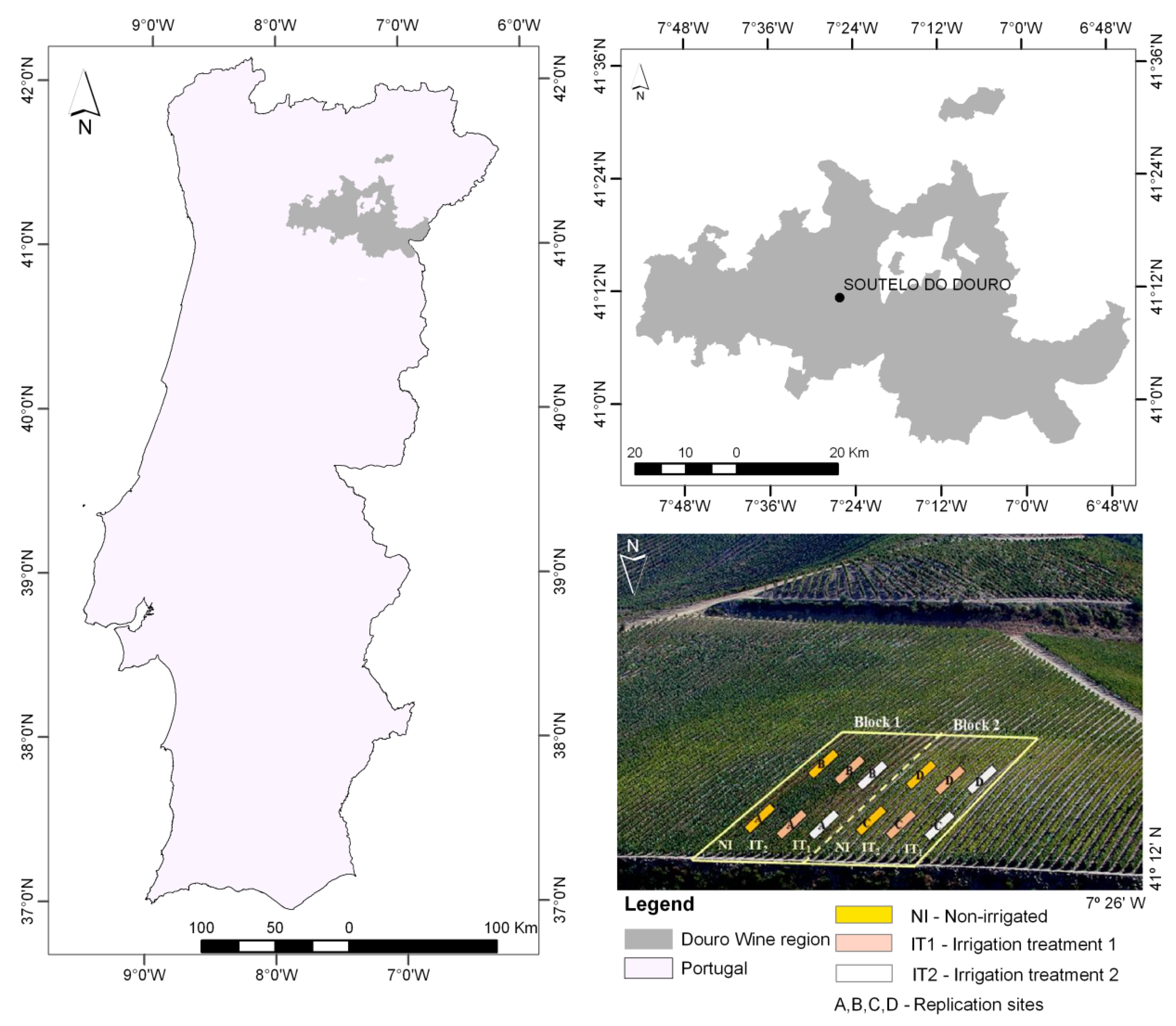
2.1. Study Area
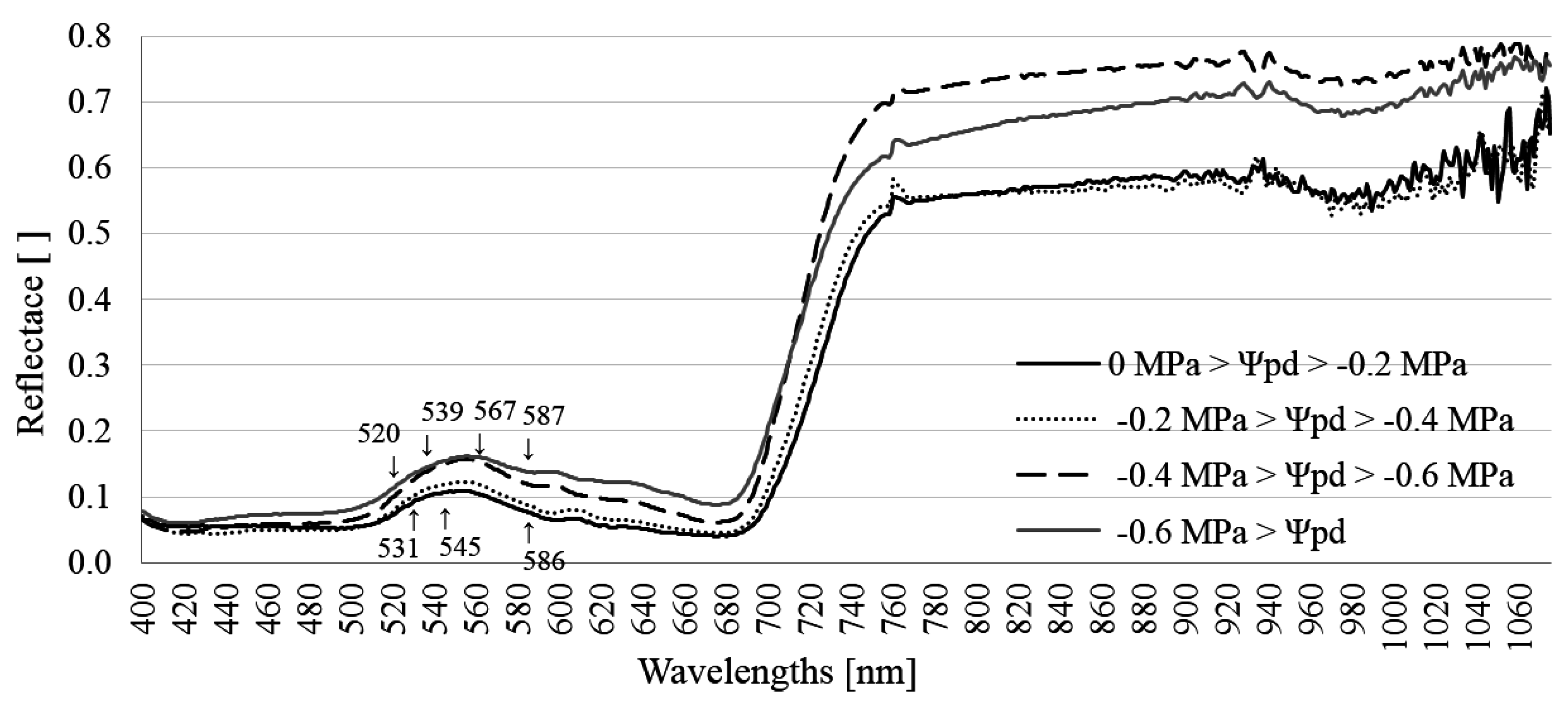
2.2. Plant Water Status and Spectral Field Measurements
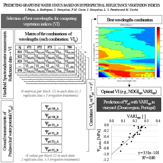
2.3. Selection of Vegetation Indices to Be Used as Predictors of Plant Water Status

| Vegetation Index | Standard Formulation | Reference |
|---|---|---|
| Visible Atmospherically Resistant Index | [14] | |
| Green Index | [48] | |
| Normalized Difference Greenness Vegetation Index | [48] | |
| Red Green Ratio Index | [49] | |
| Atmospherically resistant vegetation index (490,670,800) | [50] | |
| Simple ratio Index | [51] | |
| Normalized Difference Vegetation Index | [52] | |
| Soil Adjusted Vegetation Index | [53] | |
| Modified Soil Adjusted Vegetation Index | [54] | |
| Renormalized Difference Vegetation Index | [55] | |
| Optimal Soil Adjusted Vegetation Index | [56] | |
| Water Index | . | [23] |
| Photochemical Reflectance Index | [32] | |
| Transformed Chlorophyll Absorption in Reflectance Index | [57] | |
| Modified Chlorophyll Absorption in Reflectance Index | [21] | |
| Structure Insensitive Pigment Index | [58] | |
| Modified Red Edge Simple Ratio Index | [59] |

2.4. Statistical Analysis
- (a)
- The determination coefficient (R2) of the ordinary least-squares regression between the values of Ψpd predicted with the VI predictive equation (Ψpd VI) and measured (Ψpd obs). A determination coefficient R2 near 1.0 indicates that most of the variance of the observed values is explained by the model (predictive equation).
- (b)
- The regression coefficient (b) of the linear regression through the origin relating Ψpd VI and Ψpd obs. A value of b close to 1 indicates that the predicted values are statistically close to the observed ones.
- (c)
- The root mean square error (RMSE) that expresses the variance of residual errors, and which may vary between zero, when a perfect match would occur, and a positive value, hopefully smaller than the mean of observations; the smaller the RMSE, the better the predictive equation.
- (d)
- The average absolute error (AAE), which expresses the average size of the errors of estimate.
- (e)
- The percent bias (PBIAS) that measures the average tendency of the predicted data to be larger or smaller than their corresponding observations. Low values indicate an accurate prediction and positive or negative values indicate the occurrence of an under- or over-estimation bias.
- (f)
- The absolute differences between Ψpd VI and Ψpd obs (|Ψpd VI − Ψpd obs|) considering different classes of water deficit conditions.
- (g)
- The modelling efficiency (EF), proposed by Nash and Sutcliffe [64], that is used to determine the relative magnitude of the residual variance compared to the measured data variance. Values close to 1.0 indicate that the variance of residuals is much smaller than the variance of observations; contrarily, when EF is close to 0 or negative, this means that the mean is as good or better predictor than the model.
3. Results
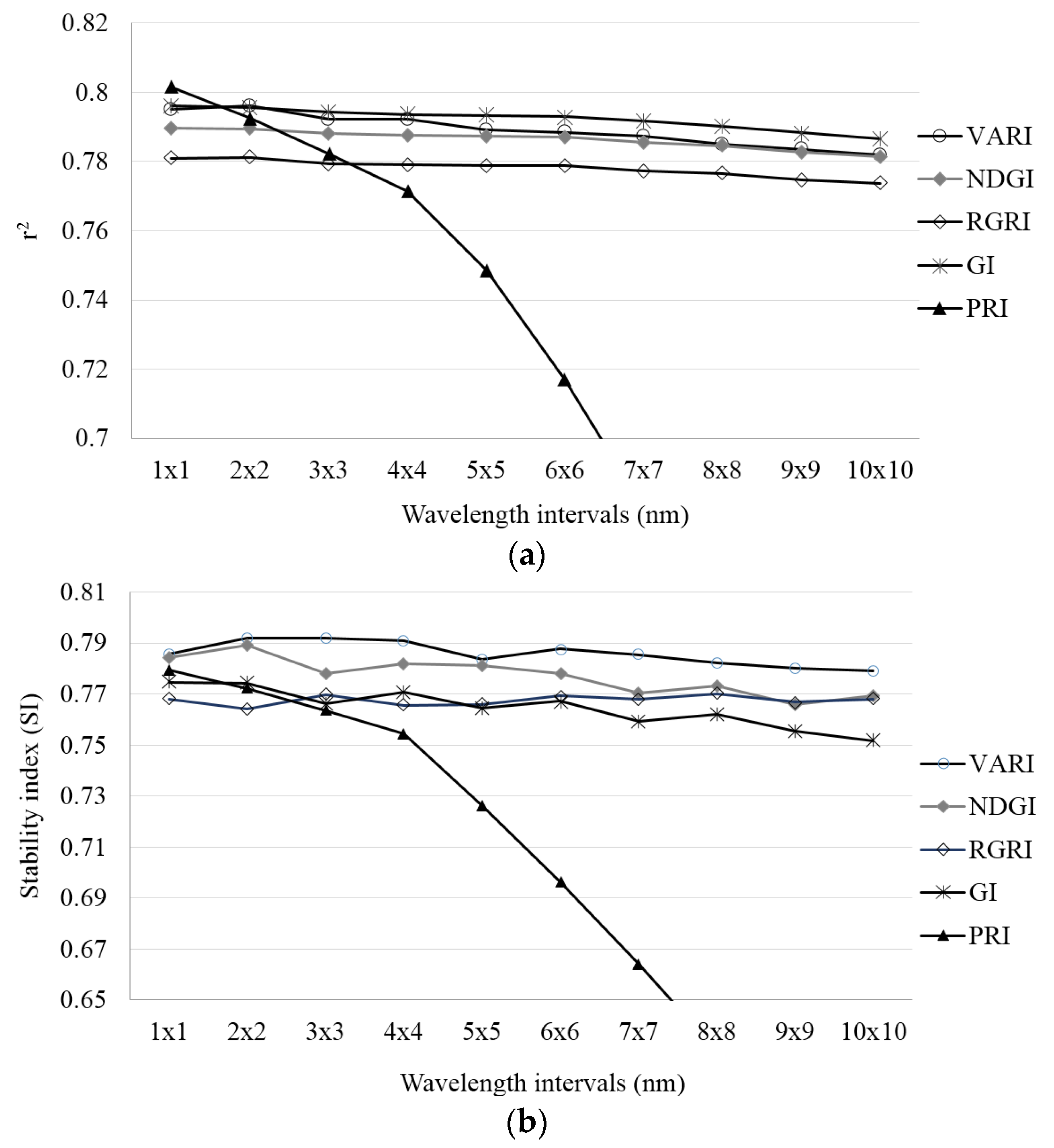
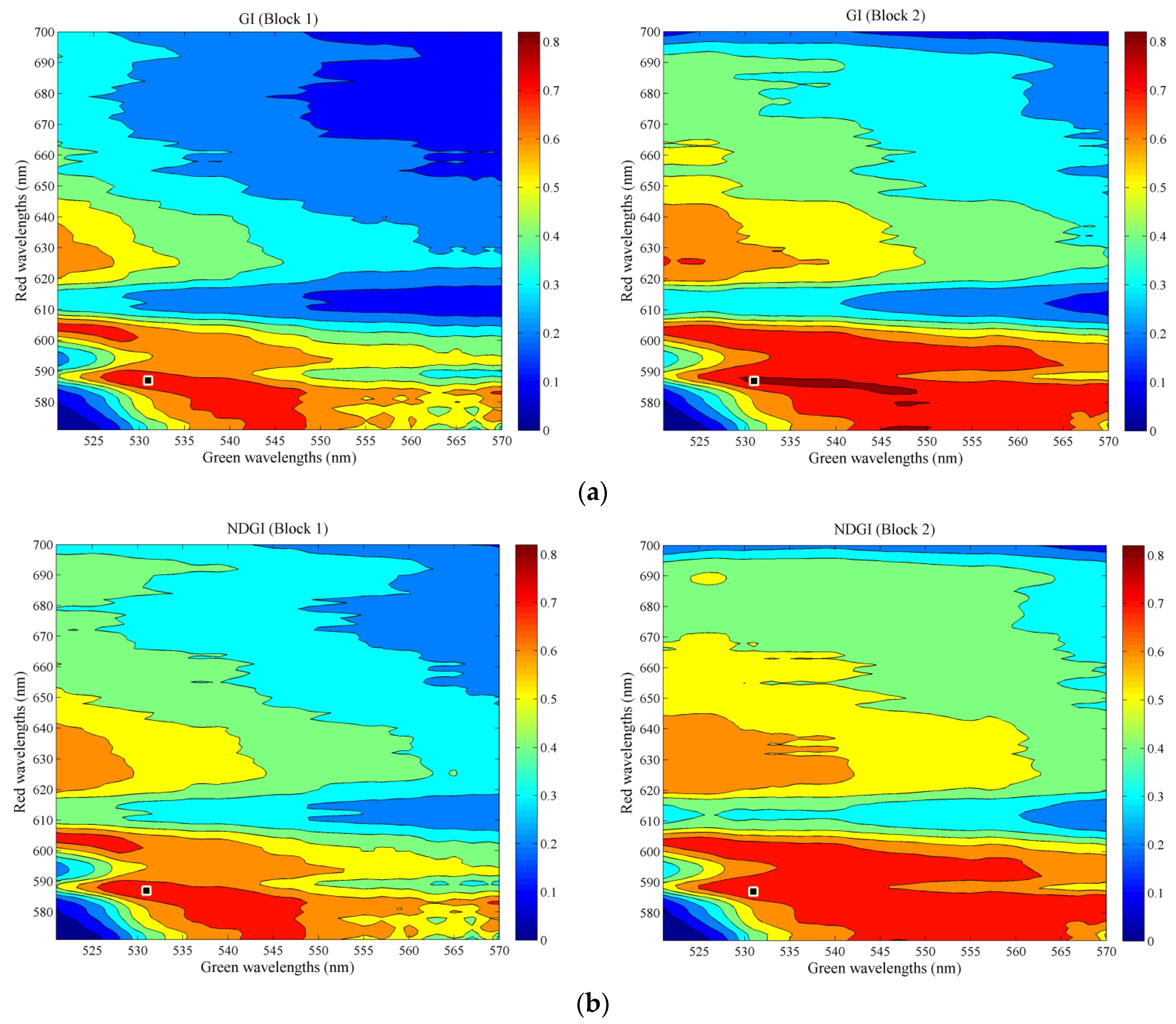
3.1. Selection of Predictors of Crop Water Status
| Vegetation Index | Standard Formulation | Optimized Formulation (1 nm Wavelengths) | |||
|---|---|---|---|---|---|
| Block 1 (n = 27) | Block 2 (n = 30) | Block 1 (n = 27) | Block 2 (n = 30) | Optimal Wavelengths | |
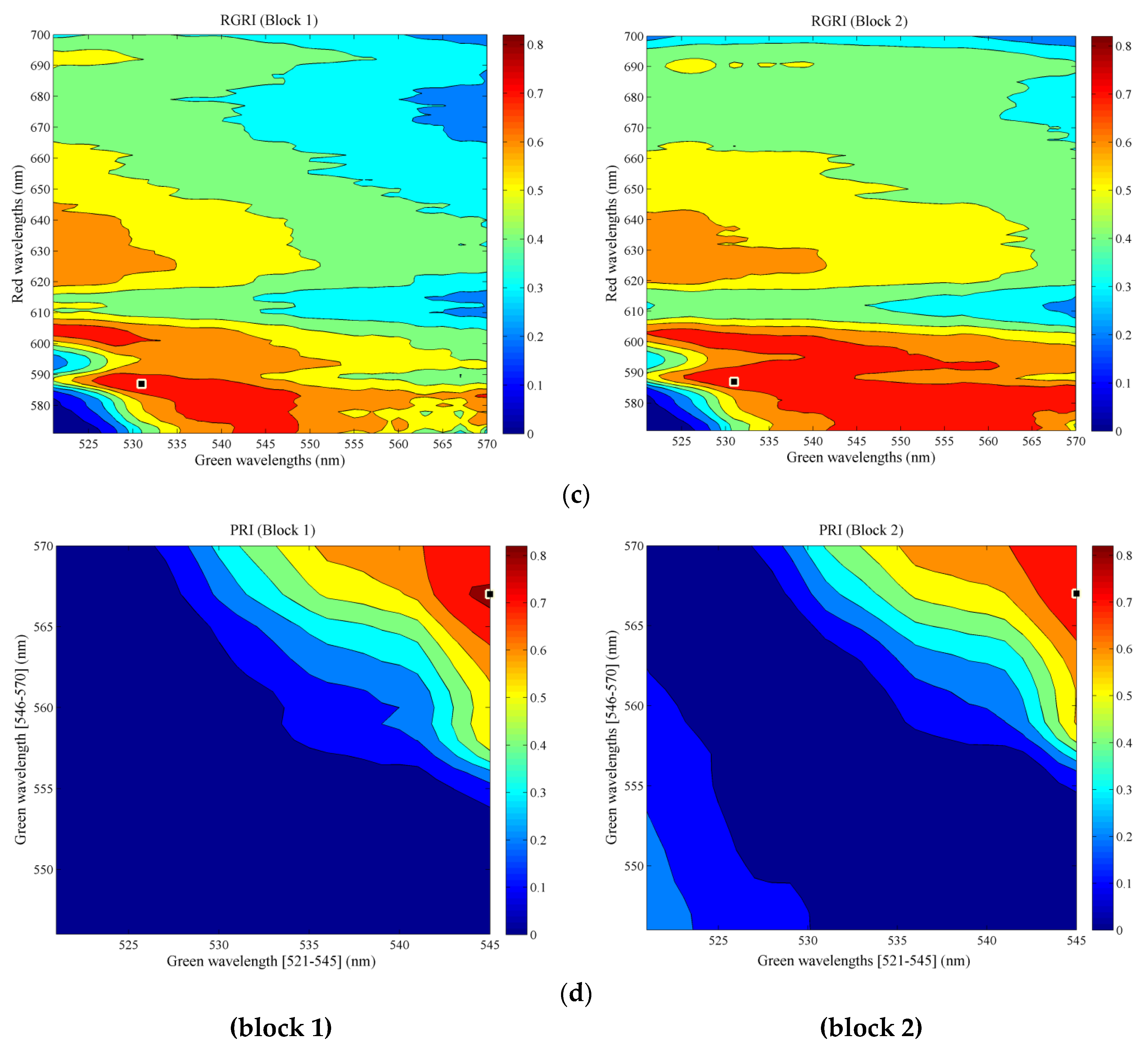
| VARI | 0.55 *** | 0.58 *** | 0.80 *** | 0.79 *** | (520; 539; 586) |
| GI | 0.37 *** | 0.51 *** | 0.78 *** | 0.81 *** | (531; 587) |
| NDGI | 0.45 *** | 0.54 *** | 0.79 *** | 0.79 *** | (531; 587) |
| PRI | 0.39 *** | 0.39 *** | 0.82 *** | 0.79 *** | (545; 567) |
| RGRI | 0.50 *** | 0.54 *** | 0.79 *** | 0.77 *** | (531; 587) |
| TCARI | 0.03 | 0.02 | 0.50 *** | 0.55 *** | (526; 682; 650) |
| MCARI | 0.01 | 0.01 | 0.59 *** | 0.61 *** | (526; 682; 645) |
| ARVI | 0.44 *** | 0.46 *** | 0.73 *** | 0.66 *** | (716; 605; 520) |
| WI | 0.00 | 0.59 *** | 0.36 *** | 0.71 *** | (943; 1038) |
| SR | 0.04 | 0.29 ** | 0.36 *** | 0.55 *** | (700; 702) |
| NDVI | 0.09 | 0.20 * | 0.36 *** | 0.55 *** | (702; 700) |
| SAVI | 0.23 * | 0.17 * | 0.42 *** | 0.44 *** | (761; 700) |
| MSAVI | 0.25 ** | 0.17 * | 0.46 *** | 0.43 *** | (761; 700) |
| RDVI | 0.22 * | 0.17 * | 0.37 *** | 0.41 *** | (761; 700) |
| SIPI | 0.50 *** | 0.35 *** | 0.64 *** | 0.56 *** | (701; 700; 426) |
| OSAVI | 0.27 ** | 0.21 * | 0.44 *** | 0.56 *** | (740; 700) |
| mRESR | 0.31 ** | 0.66 *** | 0.49 *** | 0.73 *** | (702; 700; 426) |


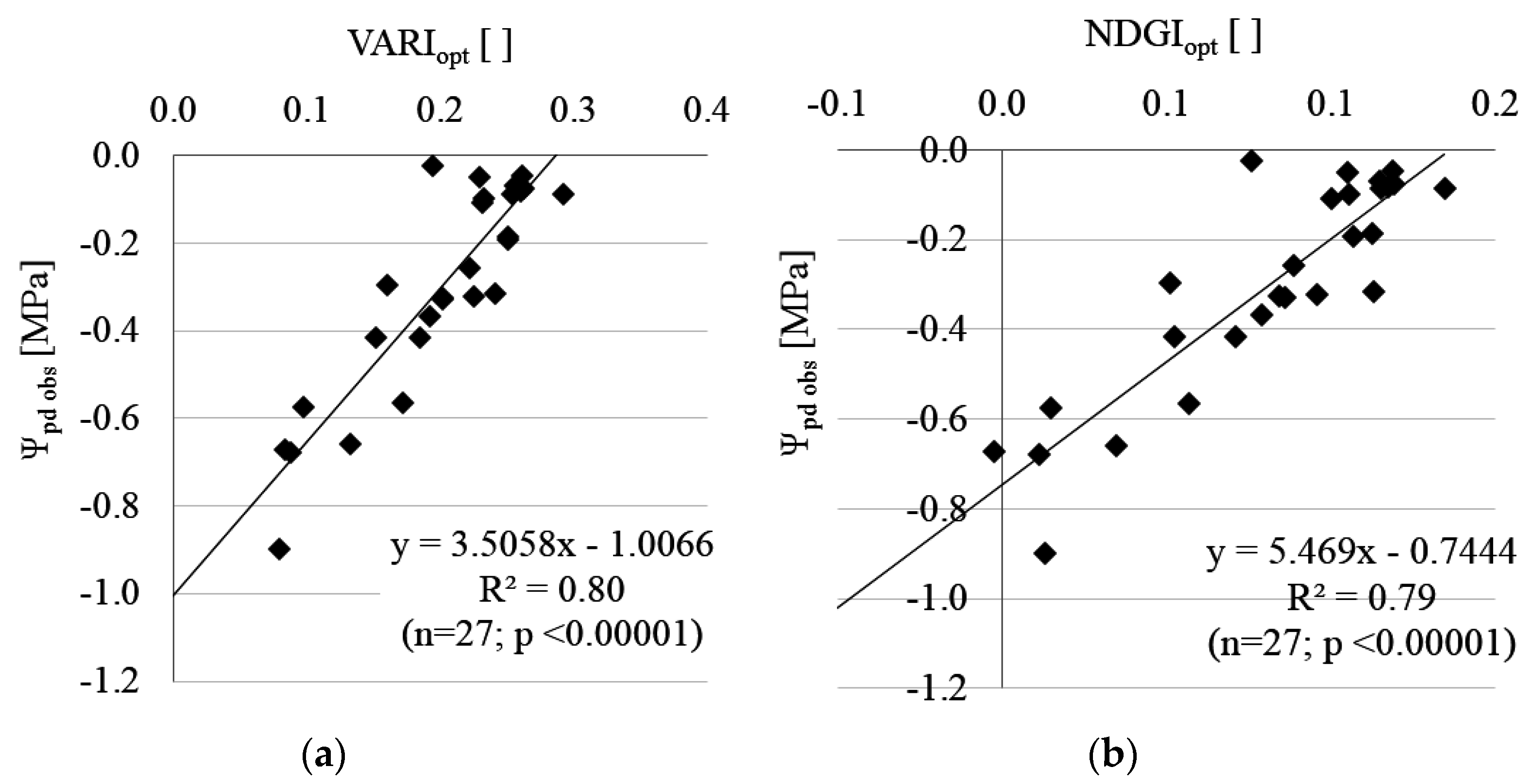
3.2. Estimation of Leaf Water Potential (Ψpd)

| Block 2 | LOO Cross-Validation | |||
|---|---|---|---|---|
| Statistics | Ψpd obs vs. Ψpd VARI | Ψpd obs vs. Ψpd NDGI | Ψpd obs vs. Ψpd VARI | Ψpd obs vs. Ψpd NDGI |
| R2 | 0.79 (p < 0.00001) | 0.79 (p < 0.00001) | 0.75 (p < 0.00001) | 0.75 (p < 0.00001) |
| b | 0.96 | 0.93 | 0.96 | 0.96 |
| RMSE (MPa) | 0.12 | 0.12 | 0.12 | 0.12 |
| AAE (MPa) | 0.097 | 0.097 | 0.101 | 0.102 |
| PBIAS (%) | 3.72 | 5.46 | −0.52 | −0.53 |
| EF | 0.76 | 0.77 | 0.75 | 0.75 |

4. Discussion
5. Conclusions
Acknowledgments
Author Contributions
Conflicts of Interest
References
- Santesteban, L.G.; Miranda, C.; Royo, J.B. Regulated deficit irrigation effects on growth, yield, grape quality and individual anthocyanin composition in Vitis vinifera L. Cv. “Tempranillo”. Agric. Water Manag. 2011, 98, 1171–1179. [Google Scholar] [CrossRef]
- Acevedo-Opazo, C.; Ortega-Farias, S.; Fuentes, S. Effects of grapevine (Vitis vinifera L.) water status on water consumption, vegetative growth and grape quality: An irrigation scheduling application to achieve regulated deficit irrigation. Agric. Water Manag. 2010, 97, 956–964. [Google Scholar] [CrossRef]
- Williams, L.E.; Araujo, F.J. Correlations among predawn leaf, midday leaf, and midday stem water potential and their correlations with other measures of soil and plant water status in Vitis vinifera. J. Am. Soc. Hortic. Sci. 2002, 127, 448–454. [Google Scholar]
- Rodríguez-Pérez, J.R.; Riaño, D.; Carlisle, E.; Ustin, S.; Smart, D.R. Evaluation of hyperspectral reflectance indexes to detect grapevine water status in vineyards. Am. J. Enol. Vitic. 2007, 58, 302–317. [Google Scholar]
- Escalona, J.M.; Fuentes, S.; Tomás, M.; Martorell, S.; Flexas, J.; Medrano, H. Responses of leaf night transpiration to drought stress in Vitis vinifera L. Agric. Water Manag. 2013, 118, 50–58. [Google Scholar] [CrossRef]
- Flexas, J.; Galmés, J.; Gallé, A.; Gulías, J.; Pou, A.; Ribas-Carbo, M.; Tomàs, M.; Medrano, H. Improving water use efficiency in grapevines: Potential physiological targets for biotechnological improvement. Aust. J. Grape Wine Res. 2010, 16, 106–121. [Google Scholar] [CrossRef]
- Rogiers, S.Y.; Greer, D.H.; Hutton, R.J.; Landsberg, J.J. Does night-time transpiration contribute to anisohydric behaviour in a Vitis vinifera cultivar? J. Exp. Bot. 2009, 60, 3751–3763. [Google Scholar] [CrossRef] [PubMed]
- Schultz, H.R.; Stoll, M. Some critical issues in environmental physiology of grapevines: Future challenges and current limitations. Aust. J. Grape Wine Res. 2010, 16, 4–24. [Google Scholar] [CrossRef]
- Fuentes, S.; de Bei, R.; Collins, M.J.; Escalona, J.M.; Medrano, H.; Tyerman, S. Night-time responses to water supply in grapevines (Vitis vinifera L.) under deficit irrigation and partial root-zone drying. Agric. Water Manag. 2014, 138, 1–9. [Google Scholar] [CrossRef]
- Serrano, L.; González-Flor, C.; Gorchs, G. Assessing vineyard water status using the reflectance based water index. Agric. Ecosyst. Environ. 2010, 139, 490–499. [Google Scholar] [CrossRef]
- Rallo, G.; Minacapilli, M.; Ciraolo, G.; Provenzano, G. Detecting crop water status in mature olive groves using vegetation spectral measurements. Biosyst. Eng. 2014, 128, 52–68. [Google Scholar] [CrossRef]
- Thenkabail, P.S.; Lyon, J.G.; Huete, A. Advances in hyperspectral remote sensing of vegetation and agricultural croplands. In Hyperspectral Remote Sensing of Vegetation; Thenkabail, P.S., Lyon, J.G., Huete, A., Eds.; CRC Press, Taylor & Francis Group: Boca Raton, FL, USA, 2012; pp. 4–35. [Google Scholar]
- Clevers, J.G.P.W.; Kooistra, L.; Schaepman, M.E. Estimating canopy water content using hyperspectral remote sensing data. Int. J. Appl. Earth Obs. Geoinf. 2010, 12, 119–125. [Google Scholar] [CrossRef]
- Gitelson, A.A.; Kaufman, Y.J.; Stark, R.; Rundquist, D. Novel algorithms for remote estimation of vegetation fraction. Remote Sens. Environ. 2002, 80, 76–87. [Google Scholar] [CrossRef]
- Viña, A.; Gitelson, A.A. Sensitivity to foliar anthocyanin content of vegetation indices using green reflectance. Geosci. Remote Sens. Lett. IEEE 2011, 8, 464–468. [Google Scholar] [CrossRef]
- Pôças, I.; Paço, T.; Paredes, P.; Cunha, M.; Pereira, L. Estimation of actual crop coefficients using remotely sensed vegetation indices and soil water balance modelled data. Remote Sens. 2015, 7, 2373–2400. [Google Scholar] [CrossRef]
- Pôças, I.; Cunha, M.; Pereira, L.S.; Allen, R.G. Using remote sensing energy balance and evapotranspiration to characterize montane landscape vegetation with focus on grass and pasture lands. Int. J. Appl. Earth Obs. Geoinf. 2013, 21, 159–172. [Google Scholar] [CrossRef]
- Jones, H.G.; Vaughan, R.A. Remote Sensing of Vegetation. Principles, Techniques, and Applications; Oxford University Press: Oxford, UK, 2010; p. 353. [Google Scholar]
- Thenkabail, P.S.; Teluguntla, P.; Gumma, M.K.; Dheeravath, V. Hyperspectral remote sensing for terrestrial applications. In Remote Sensing Handbook. Land Resources Monitoring, Modeling, and Mapping with Remote Sensing; Thenkabail, P.S., Ed.; CRC Press, Taylor and Francis Group: Boca Raton, FL, USA, 2016; pp. 201–233. [Google Scholar]
- Zarco-Tejada, P.J.; Guillén-Climent, M.L.; Hernández-Clemente, R.; Catalina, A.; González, M.R.; Martín, P. Estimating leaf carotenoid content in vineyards using high resolution hyperspectral imagery acquired from an unmanned aerial vehicle (UAV). Agric. For. Meteorol. 2013, 171–172, 281–294. [Google Scholar] [CrossRef]
- Daughtry, C.S.T.; Walthall, C.L.; Kim, M.S.; de Colstoun, E.B.; McMurtrey, J.E., III. Estimating corn leaf chlorophyll concentration from leaf and canopy reflectance. Remote Sens. Environ. 2000, 74, 229–239. [Google Scholar] [CrossRef]
- Zarco-Tejada, P.J.; González-Dugo, V.; Williams, L.E.; Suárez, L.; Berni, J.A.J.; Goldhamer, D.; Fereres, E. A PRI-based water stress index combining structural and chlorophyll effects: Assessment using diurnal narrow-band airborne imagery and the CWSI thermal index. Remote Sens. Environ. 2013, 138, 38–50. [Google Scholar] [CrossRef]
- Peñuelas, J.; Filella, I.; Biel, C.; Serrano, L.; Savé, T. The reflectance at the 950–970 nm as an indicator of plant water status. Int. J. Remote Sens. 1993, 14, 1887–1905. [Google Scholar] [CrossRef]
- Peñuelas, J.; Pinol, J.; Ogaya, R.; Filella, I. Estimation of plant water concentration by the reflectance water index WI (R900/R970). Int. J. Remote Sens. 1997, 18, 2869–2875. [Google Scholar] [CrossRef]
- Roberts, D.A.; Roth, K.L.; Perroy, R.L. Hyperspectral vegetation indices. In Hyperspectral Remote Sensing of Vegetation; Thenkabail, P.S., Lyon, J.G., Huete, A., Eds.; CRC Press, Taylor & Francis Group: Boca Raton, FL, USA, 2012; pp. 309–327. [Google Scholar]
- De Bei, R.; Cozzolino, D.; Sullivan, W.; Cynkar, W.; Fuentes, S.; Dambergs, R.; Pech, J.; Tyerman, S. Non-destructive measurement of grapevine water potential using near infrared spectroscopy. Aust. J. Grape Wine Res. 2011, 17, 62–71. [Google Scholar] [CrossRef]
- González-Fernández, A.B.; Rodríguez-Pérez, J.R.; Marcelo, V.; Valenciano, J.B. Using field spectrometry and a plant probe accessory to determine leaf water content in commercial vineyards. Agric. Water Manag. 2015, 156, 43–50. [Google Scholar] [CrossRef]
- Berni, J.A.J.; Zarco-Tejada, P.J.; Sepulcre-Cantó, G.; Fereres, E.; Villalobos, F. Mapping canopy conductance and CWSI in olive orchards using high resolution thermal remote sensing imagery. Remote Sens. Environ. 2009, 113, 2380–2388. [Google Scholar] [CrossRef]
- Sepulcre-Cantó, G.; Zarco-Tejada, P.J.; Jiménez-Muños, J.C.; Sobrino, J.A.; de Miguel, E.; Villalobos, F.J. Detection of water stress in olive orchard with thermal remote sensing imagery. Agric. For. Meteorol. 2006, 136, 31–44. [Google Scholar] [CrossRef]
- Rossini, M.; Fava, F.; Cogliati, S.; Meroni, M.; Marchesi, A.; Panigada, C.; Giardino, C.; Busetto, L.; Migliavacca, M.; Amaducci, S.; Colombo, R. Assessing canopy PRI from airborne imagery to map water stress in maize. ISPRS J. Photogramm. Remote Sens. 2013, 86, 168–177. [Google Scholar] [CrossRef]
- Behmann, J.; Steinrücken, J.; Plümer, L. Detection of early plant stress responses in hyperspectral images. ISPRS J. Photogramm. Remote Sens. 2014, 93, 98–111. [Google Scholar] [CrossRef]
- Gamon, J.A.; Penuelas, J.; Field, C.B. A narrow-waveband spectral index that tracks diurnal changes in photosynthetic efficiency. Remote Sens. Environ. 1992, 41, 35–44. [Google Scholar] [CrossRef]
- Moya, I.; Camenen, L.; Evain, S.; Goulas, Y.; Cerovic, Z.G.; Latouche, G.; Flexas, J.; Ounis, A. A new instrument for passive remote sensing: 1. Measurements of sunlight-induced chlorophyll fluorescence. Remote Sens. Environ. 2004, 91, 186–197. [Google Scholar] [CrossRef]
- Suárez, L.; Zarco-Tejada, P.J.; Sepulcre-Cantó, G.; Pérez-Priego, O.; Miller, J.R.; Jiménez-Muñoz, J.C.; Sobrino, J. Assessing canopy PRI for water stress detection with diurnal airborne imagery. Remote Sens. Environ. 2008, 112, 560–575. [Google Scholar] [CrossRef]
- Thenot, F.; Méthy, M.; Winkel, T. The photochemical reflectance index (PRI) as a water-stress index. Int. J. Remote Sens. 2002, 23, 5135–5139. [Google Scholar] [CrossRef]
- Andresen, T.; de Aguiar, F.B.; Curado, M.J. The Alto Douro wine region greenway. Landsc. Urban Plan. 2004, 68, 289–303. [Google Scholar] [CrossRef]
- Lourenço-Gomes, L.; Rebelo, J. The Alto Douro wine region world heritage site: The complexity of a preservation program. Rev. Tur. Patrim. Cultur. 2012, 10, 3–17. [Google Scholar]
- Gouveia, C.; Liberato, M.L.R.; DaCamara, C.C.; Trigo, R.M.; Ramos, A.M. Modelling past and future wine production in the portuguese Douro valley. Clim. Res. 2011, 48, 349–362. [Google Scholar] [CrossRef]
- Cunha, M.; Richter, C. Measuring the impact of temperature changes on the wine production in the Douro region using the short time Fourier transform. Int. J. Biometeorol. 2012, 56, 357–370. [Google Scholar] [CrossRef] [PubMed]
- Santos, J.A.; Grätsch, S.D.; Karremann, M.K.; Jones, G.V.; Pinto, J.G. Ensemble projections for wine production in the Douro valley of Portugal. Clim. Chang. 2013, 117, 211–225. [Google Scholar] [CrossRef]
- Figueiredo, T.; Poesen, J.; Ferreira, A.G.; Gonçalves, D. Runoff and soil loss from steep sloping vineyards in the Douro valley, Portugal: Rates and factors. In Runoff Erosion, Athens, Greece, 2013; Evelpidou, N., Cordier, S., Merino, A., Figueiredo, T.D., Centeri, C., Eds.; University of Athens: Athens, Greece, 2013; pp. 323–344. [Google Scholar]
- Cruz, J.; Pregitzer, A.; Granja, M. Douro River—A Golden Heritage; Relevo, Produção Audiovisual Lda: Porto, Portugal, 2012. [Google Scholar]
- IVDP Instituto dos Vinhos do Douro e Porto, Dados Estatísticos Sobre a Produção de Vinho do Douro e Porto na Região Demarcada do Douro. Available online: http://www.ivdp.pt/statistics (accessed on 21 July 2015).
- Jones, G.V. Climate changes and the global wine industry. In Proceedings of the 13th Australian Wine Industry Technical Conference, Adelaide, Australia, 28 July–2 August 2007.
- Alves, F.; Costa, J.; Costa, P.; Correia, C.; Gonçalves, B.; Soares, R.; Moutinho-Pereira, J. Grapevine water stress management in Douro region: Long-term physiology, yield and quality studies in cv. Touriga nacional. In Proceedings of the 18th International Symposium GiESCO, Porto, 7–11 July 2013; Portugal, Faculdade de Ciências da Universidade do Porto: Porto, Portugal, 2013. [Google Scholar]
- Scholander, P.F.; Hammel, H.T.; Bradstreet, E.D.; Hemmingsen, E.A. Sap pressure in vascular plants. Science 1965, 148, 339–346. [Google Scholar] [CrossRef] [PubMed]
- Carbonneau, A. Irrigation, vignoble et produit de la vigne. In Traité D’irrigation. Chapitre iv. Aspects Qualitatifs; Tiercelin, J.R., Ed.; Lavoisier Tec et Doc: Paris, France, 1998; pp. 257–298. [Google Scholar]
- Chamard, P.; Courel, M.F.; Docousso, M.; Guénégou, M.C.; LeRhun, J.; Levasseur, J.; Togola, M. Utilisation des bandes spectrales du vert et du rouge pour une meilleure évaluation des formations végétales actives. In Télédétection et Cartographie; AUPELF-UREF: Sherbrooke, QC, Canada, 1991; pp. 203–209. [Google Scholar]
- Gamon, J.A.; Surfus, J.S. Assessing leaf pigment content and activity with a reflectometer. New Phytol. 1999, 143, 105–117. [Google Scholar] [CrossRef]
- Kaufman, Y.J.; Tanre, D. Atmospherically resistant vegetation index (ARVI) for EOS-MODIS. Geosci. Remote Sens. IEEE Trans. 1992, 30, 261–270. [Google Scholar] [CrossRef]
- Birth, G.; McVey, G. Measuring the color of growing turf with a reflectance spectrophotometer. Agron. J. 1968, 60, 640–643. [Google Scholar] [CrossRef]
- Rouse, W.; Haas, R.; Scheel, J.; Deering, W. Monitoring vegetation systems in great plains with ERST. In Proceedings of the Third ERTS Symposium, NASA SP-351, Washington, DC, USA, 10–14 December 1973; US Government Printing Office: Washington, DC, USA, 1973; pp. 309–317. [Google Scholar]
- Huete, A.R. A soil-adjusted vegetation index (SAVI). Remote Sens. Environ. 1988, 25, 295–309. [Google Scholar] [CrossRef]
- Qi, J.; Chehbouni, A.; Huete, A.R.; Kerr, Y.H.; Sorooshian, S. A modified soil adjusted vegetation index. Remote Sens. Environ. 1994, 48, 119–126. [Google Scholar] [CrossRef]
- Roujean, J.; Breon, F. Estimating PAR absorbed by vegetation from bidirectional reflectance measurements. Remote Sens. Environ. 1995, 51, 375–384. [Google Scholar] [CrossRef]
- Rondeaux, G.; Steven, M.; Baret, F. Optimization of soil-adjusted vegetation indices. Remote Sens. Environ. 1996, 55, 95–107. [Google Scholar] [CrossRef]
- Haboudane, D.; John, R.; Millera, J.R.; Tremblay, N.; Zarco-Tejada, P.J.; Dextraze, L. Integrated narrow-band vegetation indices for prediction of crop chlorophyll content for application to precision agriculture. Remote Sens. Environ. 2002, 81, 416–426. [Google Scholar] [CrossRef]
- Peñuelas, J.; Baret, F.; Filella, I. Semi-empirical indices to assess carotenoids/chlorophyll a ration from leaf spectral reflectance. Photosynthetica 1995, 31, 221–230. [Google Scholar]
- Sims, D.A.; Gamon, J.A. Relationships between leaf pigment content and spectral reflectance across a wide range of species, leaf structures and developmental stages. Remote Sens. Environ. 2002, 81, 337–354. [Google Scholar] [CrossRef]
- Moriasi, D.N.; Arnold, J.G.; Van-Liew, M.W.; Bingner, R.L.; Harmel, R.D.; Veith, T.L. Model evaluation guidelines for systematic quantification of accuracy in watershed simulations. Trans. ASABE 2007, 50, 885–900. [Google Scholar] [CrossRef]
- Pereira, L.S.; Paredes, P.; Rodrigues, G.C.; Neves, M. Modeling malt barley water use and evapotranspiration partitioning in two contrasting rainfall years. Assessing AquaCrop and SIMDualKC models. Agric. Water Manag. 2015, 159, 239–254. [Google Scholar] [CrossRef]
- Tedeschi, L.O. Assessment of the adequacy of mathematical models. Agric. Syst. 2006, 89, 225–247. [Google Scholar] [CrossRef]
- Wang, X.; Williams, J.R.; Gassman, P.W.; Baffaut, C.; Izaurralde, R.C.; Jeong, J.; Kiniry, J.R. EPIC and APEX: Model use, calibration, and validation. Trans. ASABE 2012, 55, 1447–1462. [Google Scholar] [CrossRef]
- Nash, J.E.; Sutcliffe, J.V. River flow forecasting through conceptual models: Part 1. A discussion of principles. J. Hydrol. 1970, 10, 282–290. [Google Scholar] [CrossRef]
- Zarco-Tejada, P.J.; Berjón, A.; López-Lozano, R.; Miller, J.R.; Martín, P.; Cachorro, V.; González, M.R.; de Frutos, A. Assessing vineyard condition with hyperspectral indices: Leaf and canopy reflectance simulation in a row-structured discontinuous canopy. Remote Sens. Environ. 2005, 99, 271–287. [Google Scholar] [CrossRef]
- Gitelson, A.A. Nondestructive estimation of foliar pigment (chlorophylls, carotenoids, and anthocyanins) contents: Evaluating a semianalytical three-band model. In Hyperspectral Remote Sensing of Vegetation; Thenkabail, P.S., Lyon, J.G., Huete, A., Eds.; CRC Press: Boca Raton, FL, USA, 2012; pp. 141–165. [Google Scholar]
- Zygielbaum, A.I.; Gitelson, A.A.; Arkebauer, T.J.; Rundquist, D.C. Non-destructive detection of water stress and estimation of relative water content in maize. Geophys. Res. Lett. 2009, 36, 1–4. [Google Scholar] [CrossRef]
- Middleton, E.M.; Huemmrich, K.F.; Cheng, Y.-B.; Margolis, H.A. Spectral bioindicators of photosinthetic efficiency and vegetation stress. In Hyperspectral Remote Sensing of Vegetation; Thenkabail, P.S., Lyon, J.G., Huete, A., Eds.; CRC Press, Taylor & Francis Group: Boca Raton, FL, USA, 2012; pp. 265–288. [Google Scholar]
- Morales, C.G.; Pino, M.T.; del Pozo, A. Phenological and physiological responses to drought stress and subsequent rehydration cycles in two raspberry cultivars. Sci. Hortic. 2013, 162, 234–241. [Google Scholar] [CrossRef]
- Guyot, G. Optical properties of vegetation canopies. In Applications of Remote Sensing in Agriculture; Steven, M.D., Clark, J.A., Eds.; Butterworths: London, UK, 1990; pp. 19–43. [Google Scholar]
- Perry, E.M.; Roberts, D.A. Sensitivity of narrow-band and broad-band indices for assessing nitrogen availability and water stress in an annual crop. Agron. J. 2008, 100, 1211–1219. [Google Scholar] [CrossRef]
- Stagakis, S.; González-Dugo, V.; Cid, P.; Guillén-Climent, M.L.; Zarco-Tejada, P.J. Monitoring water stress and fruit quality in an orange orchard under regulated deficit irrigation using narrow-band structural and physiological remote sensing indices. ISPRS J. Photogramm. Remote Sens. 2012, 71, 47–61. [Google Scholar] [CrossRef]
- Sun, P.; Grignetti, A.; Liu, S.; Casacchia, R.; Salvatori, R.; Pietrini, F.; Loreto, F.; Centritto, M. Associated changes in physiological parameters and spectral reflectance indices in olive (Olea europaea L.) leaves in response to different levels of water stress. Int. J. Remote Sens. 2008, 29, 1725–1743. [Google Scholar] [CrossRef]
- Gitelson, A.A.; Kaufman, Y.J.; Merzlyak, M.N. Use of a green channel in remote sensing of global vegetation from EOS-MODIS. Remote Sens. Environ. 1996, 58, 289–298. [Google Scholar] [CrossRef]
- Carter, G.A.; Knapp, A.K. Leaf optical properties in higher plants: Linking spectral characteristics to stress and chlorophyll concentration. Am. J. Bot. 2001, 88, 677–684. [Google Scholar] [CrossRef] [PubMed]
- Hernández-Clemente, R.; Navarro-Cerrillo, R.M.; Suárez, L.; Morales, F.; Zarco-Tejada, P.J. Assessing structural effects on PRI for stress detection in conifer forests. Remote Sens. Environ. 2011, 115, 2360–2375. [Google Scholar] [CrossRef]
- Zarco-Tejada, P.J.; González-Dugo, V.; Berni, J.A.J. Fluorescence, temperature and narrow-band indices acquired from a UAV platform for water stress detection using a micro-hyperspectral imager and a thermal camera. Remote Sens. Environ. 2012, 117, 322–337. [Google Scholar] [CrossRef]
- Clevers, J.G.P.W.; van der Heijden, G.W.A.M.; Verzakov, S.; Schaepman, M.E. Estimating Grassland Biomass Using SVM Band Shaving of Hyperspectral Data. Photogram. Eng. Remote Sens. 2007, 73, 1141–1148. [Google Scholar] [CrossRef]
- Atzberger, C.; Guérif, M.; Baret, F.; Werner, W. Comparative analysis of three chemometric techniques for the spectroradiometric assessment of canopy chlorophyll content in winter wheat. Comput. Electron. Agric. 2010, 73, 165–173. [Google Scholar] [CrossRef]
© 2015 by the authors; licensee MDPI, Basel, Switzerland. This article is an open access article distributed under the terms and conditions of the Creative Commons by Attribution (CC-BY) license (http://creativecommons.org/licenses/by/4.0/).
Share and Cite
Pôças, I.; Rodrigues, A.; Gonçalves, S.; Costa, P.M.; Gonçalves, I.; Pereira, L.S.; Cunha, M. Predicting Grapevine Water Status Based on Hyperspectral Reflectance Vegetation Indices. Remote Sens. 2015, 7, 16460-16479. https://doi.org/10.3390/rs71215835
Pôças I, Rodrigues A, Gonçalves S, Costa PM, Gonçalves I, Pereira LS, Cunha M. Predicting Grapevine Water Status Based on Hyperspectral Reflectance Vegetation Indices. Remote Sensing. 2015; 7(12):16460-16479. https://doi.org/10.3390/rs71215835
Chicago/Turabian StylePôças, Isabel, Arlete Rodrigues, Sara Gonçalves, Patrícia M. Costa, Igor Gonçalves, Luís S. Pereira, and Mário Cunha. 2015. "Predicting Grapevine Water Status Based on Hyperspectral Reflectance Vegetation Indices" Remote Sensing 7, no. 12: 16460-16479. https://doi.org/10.3390/rs71215835