Development of Dense Time Series 30-m Image Products from the Chinese HJ-1A/B Constellation: A Case Study in Zoige Plateau, China

Abstract

Time series remote sensing products with both fine spatial and dense temporal resolutions are urgently needed for many earth system studies. The development of small satellite constellations with identical sensors affords novel opportunities to provide such kind of earth observations. In this paper, a new dense time series 30-m image product was proposed respectively based on an 8-day, 16-day and monthly composition. The products were composited by the Charge Coupled Device (CCD) images from the 2-day revisit small satellite constellation for environmental monitoring and disaster mitigation of China (HJ-1A/B). Taking the Zoige plateau in China as a case area where it is covered by highly heterogeneous vegetation landscapes, a detailed methodology was introduced on how to use 183 scenes of CCD images in 2010 to create composite products. The quality of the HJ CCD composites was evaluated by inter-comparison with the monthly 30-m global Web-Enabled Landsat Data (WELD), 16-day 500-m MODIS NDVI, and 8-day 500-m MODIS surface reflectance products. Results showed that the radiometric consistency between HJ and WELD composited Top Of Atmosphere (TOA) reflectance was in good agreement except for May, June, July and August when more clouds and invalid data gaps appeared in WELD. Visual assessment and temporal profile analysis also revealed that HJ possessed better visual effects and temporal coherence than that of WELD. The comparison between HJ and MODIS products indicated that HJ composites were radiometrically consistent with MODIS products over areas consisting of large patches of homogeneous surface types, but can better reflect the detailed spatial differences in regions with heterogeneous landscapes. This paper highlights the potential of compositing HJ-1A/B CCD images, allowing for providing a cloud free, time-space consistent, 30-m spatial resolution, and dense in time series image product. Meanwhile, the proposed products could also be treated as a reference to generate regional or even global composited products for the on-going satellite constellations and even for the forthcoming satellite missions such as Sentinel-2A/B.

1. Introduction

Dense time series (e.g., annual, monthly, weekly) satellite datasets are crucial for monitoring land surface dynamics (e.g., intra-seasonal ecosystem variations). Monthly or sub-monthly satellite datasets have been developed at moderate (>250 m) or coarser spatial resolutions [1,2]. However, pixels in these coarse resolution images are often a mixture of various land cover types [3,4]. Finer spatial resolutions (e.g., 30 m) and dense time series satellite datasets are urgently required to provide adequate spatial details for many surface phenomena [5,6,7,8,9,10].

Temporal composition methods can select the optimum observation over the same geographical region from multi-temporal images in a certain time window based on different user-defined rules [11,12,13,14]. In recent years, the temporal composition methods are gradually adopted for the composition of fine spatial resolution images to generate cloud-free time series datasets [11,15,16,17,18,19]. The Web-Enabled Landsat Data (WELD) project provides a good framework for producing composites at 30-m spatial resolution and monthly, seasonal, annual time intervals using Landsat 7 Enhanced Thematic Mapper Plus (ETM+) data [15]. The WELD data have been successfully employed in many studies, such as the crop field extraction and land cover change monitoring for the conterminous United States (CONUS) [20,21,22]. Based on the success of the CONUS WELD products, the WELD processing is being expanded to the global scale to provide the monthly and annual Landsat 30 m information for six three-year epochs spaced every five years from 1985–2010 [18]. Similar Landsat-based compositing has also been carried out across the entire Carpathians and Canada [11,19]. However, because of the frequent cloud contamination and the poor atmospheric conditions, the comparatively infrequent 16-day repeat of the current Landsat system does not provide adequate observations for producing gap free clear view composites at monthly or sub-monthly intervals.

Satellites or constellations with short revisit periods (e.g., 2–4 days) and fine spatial resolution sensors, which were already on orbit (e.g., HJ-1A/B, Sentinel-2A) or will be launched (e.g., Sentinel-2B), create new opportunities to generate the composites at fine spatial resolution and dense time series. A pair of Chinese HJ-1 (Huanjing (HJ), which means environment in Chinese) optical satellites, launched in 2008 and named HJ-1A and HJ-1B, provides 30-m observations every two days [23,24,25]. The HJ-1A and HJ-1B are distributed with a 180 degrees phase difference in the same orbital plane to enhance the temporal resolution. The revisit period of a single satellite in the HJ1-A/B constellation is four days, and therefore two optical satellites can obtain the global observation data within two days [26,27]. Such a high observation frequency allows generation of 30-m composites at monthly or even weekly intervals.

However, compositing using standard HJ imagery is infeasible because they are not orthorectified and hence have considerable geolocation errors. Cloud masking can also be challenging due to lack of thermal band and shortwave infrared band. The authors addressed both issues in previous studies where automated approaches were developed for orthorectifying HJ images to achieve sub-pixel geolocation accuracies and for masking cloud in those images [26,28]. Based on those approaches, this study demonstrates the feasibility of using HJ images to create composites in the Zoige plateau in China, and provide a comprehensive assessment of the quality of those composites. The rest of the paper is structured as follows: Section 2 describes the study area, HJ-1A/B satellites, sensors and data used for the compositing. Section 3 presents the preprocessing, compositing and quality assessment methods for the original data and composite results. Section 4 shows the results of compositing and evaluation by comparison with other sensors. Section 5 discusses the merits and limitations of the proposed methods, potential applications of the products, as well as the potential for the development of dense time series fine spatial resolution products by new constellations. Section 6 presents the conclusions.

2. Study Area and Data

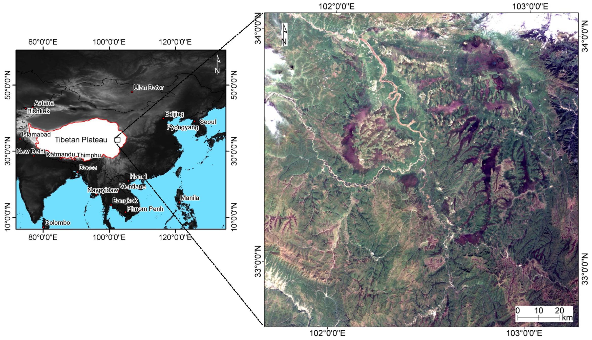
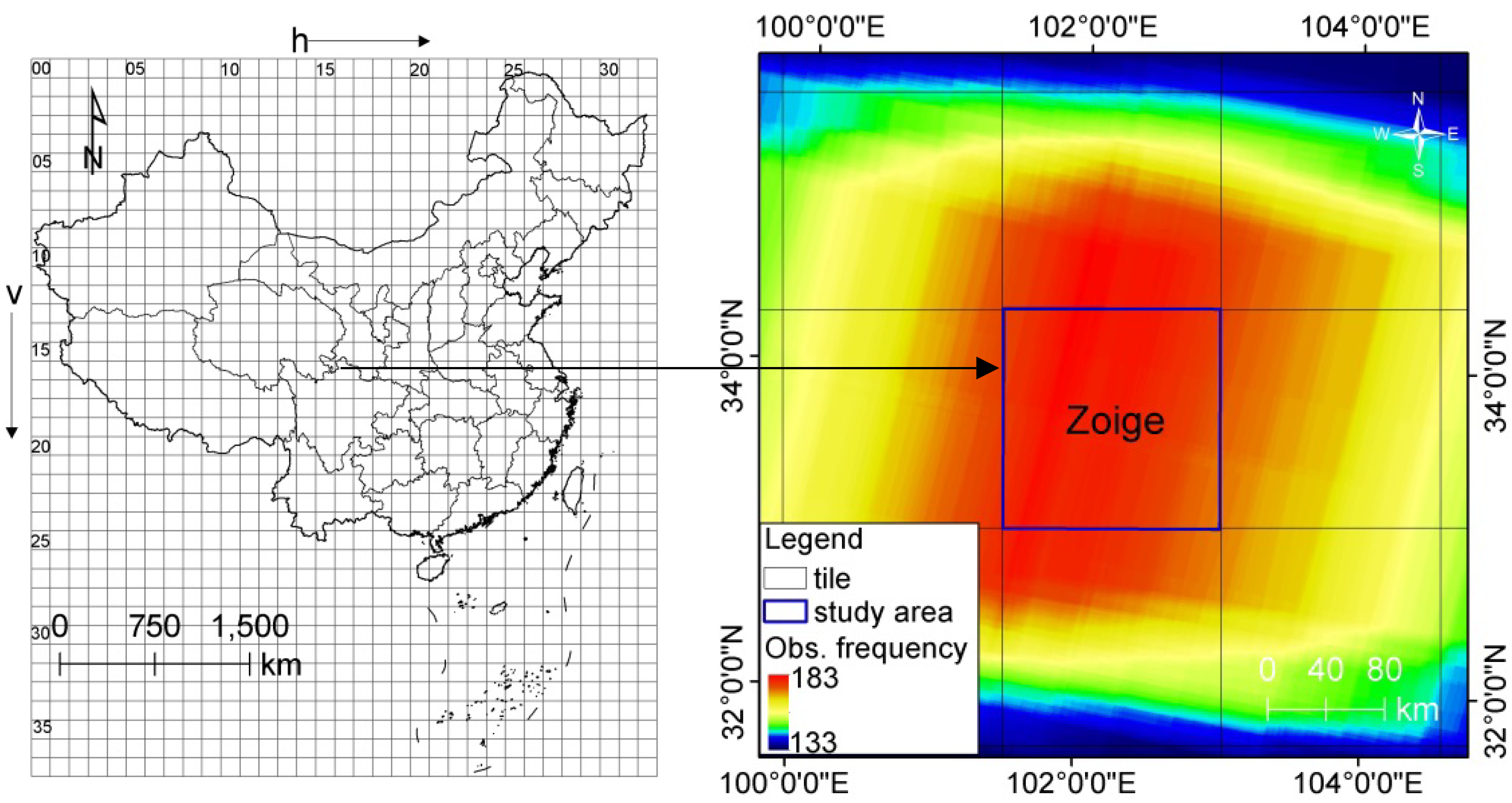
2.1. Study Area

Located at the eastern edge of Qinghai-Tibet plateau, the Zoige Plateau is covered by the largest area of peat wetlands in the world [29]. It extends from 102.00°E to 103.50°E and from 33.00°N to 34.35°N, with the average altitude of 3500 m. The climate in the Zoige plateau is cold and wet, with an annual mean temperature of 0.7 °C–3.3 °C. The mean annual precipitation recorded by the nearby Zoige meteorological station (at 3439 m a.s.l) is 648.5 mm during the period 1971–2000. Most of the precipitation falls as rain during the summer months (June–September), owing to the influence of Asian summer monsoons [30]. Because of the concentrated precipitation during this period, it is difficult to acquire the clear-sky satellite imagery, especially for the infrequent revisit satellites such as Landsat. Besides, the water levels of wetland area on the Zoige Plateau manifest substantial seasonal variations, primarily in response to precipitation events. The seasonal variation of surface water aggravates the complexity of the land surface of this area. Because of the difficulty to obtain clear-sky satellite imagery and the highly heterogeneous land surface on the Zoige Plateau, it is typical and suitable to test the quality of the composited product. An area of about 22,500 km² (150 km × 150 km) in the Zoige plateau is selected as the case study area (Figure 1). The study area is mainly covered by grassland, meadow, swamp meadow and peat land [31].

Figure 1. Location of the study area. The satellite image on the left is the subset of HJ1B CCD2 image acquired on 16 August 2010 shown with true color compositing (bands 3, 2, 1 in red, green and blue).

Figure 1. Location of the study area. The satellite image on the left is the subset of HJ1B CCD2 image acquired on 16 August 2010 shown with true color compositing (bands 3, 2, 1 in red, green and blue).

2.2. HJ-1A/B Overview

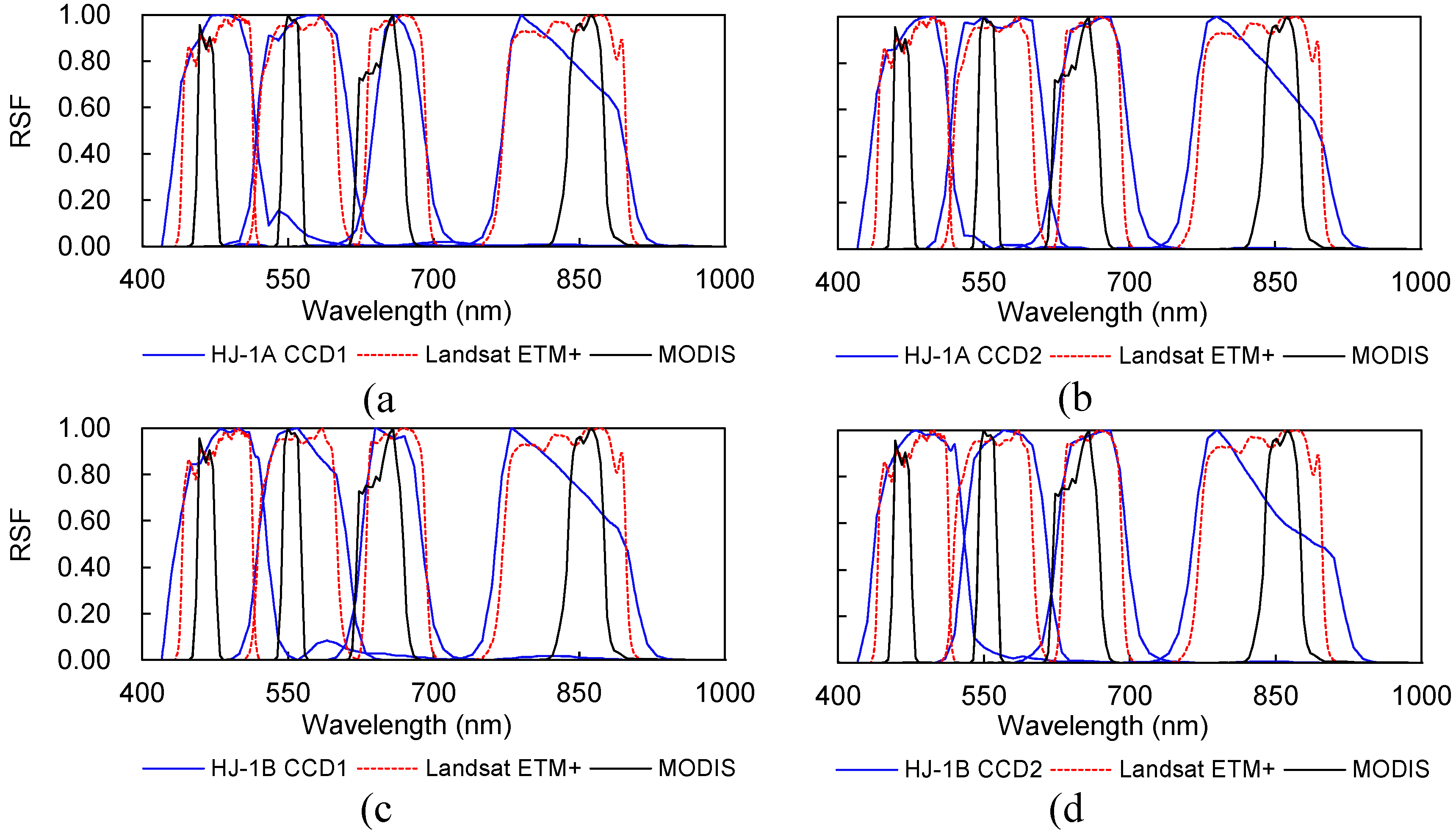
The HJ-1 constellation contains two optical satellites (HJ-1A/B, launched in September 2008). The primary goal of the optical satellites HJ-1A/B is to revisit any place in the world within two days for environmental and disaster monitoring [26]. To achieve the designed revisit frequency, HJ-1A/B were distributed in the same altitude and orbit plane, with a phase delay of 180 degrees [25]. The orbit of HJ-1A/B is sun-synchronous circular orbit at 649.093 km altitude with a 10:30 a.m. ± 30 min descending node [32]. This satellite passing time was selected as the best compromise between minimizing cloud cover and ensuring suitable sun illumination. It is also close to the Landsat local overpass time and matches that of Terra MODIS. The HJ-1A/B has a global positioning system onboard to measure the exterior orientation, which can achieve systematic geometric location accuracy of 10–20 pixels.

2.2.1. Sensors

The payload of both HJ-1A and 1B includes two identical wide-coverage multi-spectral CCD cameras. The two CCD cameras were placed symmetrically to each other and the satellite nadir point. The placement enables the two CCD cameras to equally divide the Field Of View (FOV) and observe the earth side by side. The swath width of a single HJ-1A/B camera is 360 km, while the combination of two cameras obtains a swath width of 700 km. The spatial resolution of the CCD image (referred to as HJ-1A/B images in the following) is 30 m, with three visible bands (430–520 nm, 520–600 nm, 630–690 nm) and one near-infrared band (760–900 nm) [27]. The wide coverage, fine spatial resolution and high observation frequency of HJ-1A/B images enable them to capture the rapid changes of the land surface. Table 1 briefly outlines a comparison between HJ-1A/B and Landsat TM/ETM. For details about the imaging mechanism of HJ-1A/B, see [26].

Table 1. Comparison of the characteristics between HJ-1A/B CCD and Landsat TM/ETM.

--	HJ-1A/B CCD	Landsat TM/ETM
Spatial resolution (m)	30	30
Spectral bands	4	7
Revisiting period (days)	2	16
Central wavelength (nm)	475; 560; 660; 830	485; 565; 665; 820; 1650; 2190; 11,400
Field of view (km)	360 (700 for 2 CCD)	180
Launch date	2008	1984 Landsat 5; 1999 Landsat 7

Table 1. Comparison of the characteristics between HJ-1A/B CCD and Landsat TM/ETM.

--	HJ-1A/B CCD	Landsat TM/ETM
Spatial resolution (m)	30	30
Spectral bands	4	7
Revisiting period (days)	2	16
Central wavelength (nm)	475; 560; 660; 830	485; 565; 665; 820; 1650; 2190; 11,400
Field of view (km)	360 (700 for 2 CCD)	180
Launch date	2008	1984 Landsat 5; 1999 Landsat 7

Figure 2 showed the relative Spectral Response Functions (SRF) for the equivalent reflective bands of ETM+, four HJ CCD cameras and MODIS. The central wavelength and band width between HJ CCD and Landsat ETM+ are very close. However, the SRF of MODIS is markedly narrower than that of the corresponding ETM+ and HJ CCD bands.

Figure 2. Relative spectral response functions (RSF) for HJ-1A/B CCD cameras ((a–d) are HJ-1A CCD1, HJ-1A CCD2, HJ-1B CCD1, HJ-1B CCD2, respectively), Landsat 7 Enhanced Thematic Mapper Plus (ETM+) and MODIS.

Figure 2. Relative spectral response functions (RSF) for HJ-1A/B CCD cameras ((a–d) are HJ-1A CCD1, HJ-1A CCD2, HJ-1B CCD1, HJ-1B CCD2, respectively), Landsat 7 Enhanced Thematic Mapper Plus (ETM+) and MODIS.

2.2.2. Data

The HJ-1A/B images can be obtained through the China Centre for Resources Satellite Data and Application (CRESDA) website for free, and the relevant information is available at [33] with the interface in English. The images distributed by CRESDA were Level 2 products (after systematic geometric calibration). The metadata and observation azimuth information can also be obtained together with the imagery. Because of the wide coverage of HJ-1A/B image (i.e., 360 km), the overlapping area of adjacent orbit is very large, with an overlapping rate of nearly 87.1% at the equatorial regions [28]. The high overlap rate means that images from adjacent orbits can also be used for the image composition. In this paper, in total, 183 scenes of images from the year 2010 with the paths 14–19 and row 76 were selected for the study area.

3. Methodology

3.1. Data Pre-Processing

Radiometric calibration converts Digital Numbers (DN) recorded in multi-spectral images into radiance and Top Of Atmosphere (TOA) reflectance. It is a fundamental process to eliminate the influence of the attenuation of the sensor photoelectric system [15]. It is especially important for images acquired from the constellation, because of the different attenuation rates of sensors [28]. The radiometric calibration of HJ-1A/B images was conducted by using Equation (1) to Equation (3) [34].

$$L_{\lambda }=\frac{DN}{G}+B$$

(1)

$$R_{\lambda }=\frac{\pi \times L_{\lambda }\times d_r^2}{ESU{N}_{\lambda }\times \cos \theta }$$

(2)

$$d_r=1+0.033\cos \left(DOY\cdot \frac{2\pi }{365}\right)$$

(3)

where, L_λ is the upward radiance (W·m⁻²∙sr⁻¹∙μm⁻¹), G (W⁻¹∙m²∙sr∙μm) is the gain of the absolute calibration coefficient, B (W∙m⁻²∙sr⁻¹∙μm⁻¹) is the calibration offset, ESUN_λ (W∙m⁻²∙μm⁻¹) is the solar exo-atmospheric spectral irradiance, θ is the solar zenith angle, d_r is the solar-terrestrial astronomical unit distance, and the Day of the Year (DOY). The annual calibration coefficients for Esun, G and B can be obtained from the website of CRESDA.

Sub-pixel geolocation accuracy is required to generate composites [35]. Using the auto-registration and orthorectification algorithm for HJ-1A/B images [26], geometric registration and orthorectification were carried out for all the acquired HJ-1A/B images. Using the Global Land Survey (GLS) Landsat images from the year 2005 with geolocation error less than 30 m as base images [36], the HJ-1A/B geometric registration algorithm employed the area-based matching method to automatically select tie points between the base and HJ-1A/B images. The elevation data from the Shuttle Radar Topography Mission (SRTM) with spatial resolution of 90 m was used to correct the parallax error due to the local topographic relief. For the images with the cloud cover, the distribution of control points selected by the auto-algorithm will be uneven, and therefore the geometric residuals might still be bigger than ones in the cloudless images. More control points in these images were selected by hand so that the final geometric residuals of all the images met the requirement for sub-pixel geometric accuracy.

Cloud masking for all of the images has been implemented according to [28,37]. The cloud detection algorithm was designed to take full advantage of the temporal and spatial contextual information to overcome the shortcomings of the limited spectral bands. The algorithm consisted of three major stages, which were the initial spectral text, the multi-temporal difference and the synthetic texture information test. The initial spectral test was used for detecting both clouds and bright pixels (such as snow) together based on the whiteness and haze optimized transformation spectral tests [38,39]. Then, the spectral differences between the HJ-1A/B images and a cloud-free reference image were calculated to discriminate most cloud from those bright pixels. In the third stage, the synthetic spatial texture information calculated from the distance of regional covariance matrix (RCM) was used to correct the commission and omission errors. Cloud shadow was detected using a geometry-based cloud shadow projection method proposed in [13]. In this method, cloud shadow was detected based on the shadow physical characteristics (scattering differences between the short wavelength and NIR) combined with the geometry. Since there was no well-accepted atmospheric correction method available for HJ-1A/B images, no atmospheric correction was performed.

3.2. Compositing Method

3.2.1. Tiling

Considering the orbit deviation and perturbation factors, the tile with fixed dimension (number of rows and columns) was generated for the compositing. On the one hand, the ground trace of the HJ-1A/B normally deviates toward the west within the nadir trace revisit period [28]. The deviation makes the selection of time series images that totally cover the same area difficult. On the other hand, due to the effects of atmospheric drag perturbation, non-spherical gravitational perturbation of earth and lunar-solar perturbations, the satellite orbit will deviate from the design orbit over a period of time [40]. The perturbations make the structure of the constellation unbalanced and affects the phase difference between satellites, which further made the ground trace overlapping irregular [41].

Data volume of a single file was considered to determine the tile dimension. The tile was finally determined as 5000 pixels × 5000 pixels to ensure the manageable file sizes. Figure 3 illustrated the generated tile grid system for China (left) and the standard tile quoted in this paper (right). The tile for China was generated in this paper for the purpose of selecting standard tiles of the case area. It was generated from the upper left coordinate of China in 150 km × 150 km and was defined in the Albers Equal Area projection. The color gradient at the right side represented the observation frequency of all images used in this study. The majority of the study area had 180 or more acquisitions over one year.

Figure 3. The tile coordinate scheme of China (left) and the observation frequency of HJ1-A/B for the study area in the year 2010 (right). The tiles are generated in this paper from the upper left coordinate of China in 150 km × 150 km and are defined in the Albers Equal Area projection. The color gradient represents the observation frequency of all the HJ-1A/B imagery from paths 14–19, row 76.

Figure 3. The tile coordinate scheme of China (left) and the observation frequency of HJ1-A/B for the study area in the year 2010 (right). The tiles are generated in this paper from the upper left coordinate of China in 150 km × 150 km and are defined in the Albers Equal Area projection. The color gradient represents the observation frequency of all the HJ-1A/B imagery from paths 14–19, row 76.

3.2.2. Image Composition Algorithm

In this paper, the constrained view angle-maximum value composite algorithm (CV-MVC) inherited from MODIS Vegetation Index (VI) product was used for compositing of H1A/B products. It was chosen for two reasons. Firstly, one of the purposes of this study is to exam the capability of the composites for providing spatio-temporal details for the high heterogeneous land surface on Zoige Plateau. The CV-MVC method is helpful for the obtaining of the optimum vegetation observation and eliminating the terrain shadow and cloud shadow to some extent [15]. On the other hand, since the swath width of HJ-1A/B images are large and the CCD camera is side viewing [26], the CV-MVC algorithm is also helpful for minimizing the view angle effects and, consequently, BRDF related issues for compositing of HJ-1A/B products to some extent [42].

The cloud mask generated in Section 3.1 was firstly used to exclude cloud contaminated pixels. Then, all the cloud-free HJ-1A/B observations within the time window were counted. If more than two cloud-free observations existed, observations closest to nadir view between the two highest NDVI pixels will then be selected to represent the pixel in the composite cycle. If only one cloud-free observation was in the time series, the cloud-free observation should be directly taken as the output. If all the observations are cloudy, the pixel with the largest NDVI will be selected as the output, and the pixel will still be marked as cloud in the cloud mask layer.

Three temporal intervals, which are 8-day, 16-day and one month were set to generate the HJ-1 composites. Ideally, there will be 4 and 8 observations within an 8-day and 16-day composition period, respectively. However, the number of observations is not enough to conduct the reliable BRDF correction using to a semi-physical BRDF model such as Walthall model [43]. Therefore, the BRDF effects are not corrected in the current method (to be discussed in detail in Section 5).

3.3. Quality Assessment

The quality of the HJ composites were evaluated by inter-comparison with existing well validated Landsat WELD and MODIS products. Two kinds of comparison were considered. One comparison was that HJ composites were directly compared with WELD to evaluate the radiometric consistency under the same spatial and temporal resolution. The other was that HJ composites were indirectly compared with MODIS products under the same temporal but different spatial resolution. This scheme was performed by evaluating the visual consistency with the 500-m 8-day MODIS reflectance product (MOD09A1) and the NDVI consistency with 500-m 16-day MODIS NDVI product (MOD13A1).

3.3.1. Comparison between HJ Composites and WELD Products

The monthly WELD Version 2.2 products for the year 2010 were obtained from the USGS National Center for Earth Resources Observation and Science (EROS) [44]. WELD products were systematically composited from 30 m Landsat ETM+ images to provide consistent data that can be used to derive land cover as well as biophysical products [15]. The WELD Version 2.2 products are defined in the equal area sinusoidal projection in a global non-overlapping grid of 5295 × 5295 30-m pixel tiles that are nested to the standard MODIS land product tiles.

The Landsat ETM+ reflective wavelength bands Blue, Green, Red, NIR (Table 1) and the TOA NDVI were used for comparison. All WELD products in the corresponding HJ composites regions from the year 2010 were downloaded via USGS EROS. Pixels flagged as cloud either in WELD ACCA state, DT cloud state, or HJ cloud mask were all removed before the comparison.

3.3.2. Comparison between HJ Composites and MODIS Products

The quality assessments for 8-day and 16-day HJ composites are relatively difficult because of the lack of similar spatio-temporal resolution composite products. In this paper, the 8-day 500-m MODIS MOD09A1 and 16-day 500-m MOD13A1 products were used for comparison. Due to the difference between TOA reflectance and surface reflectance, the comparison between the 8-day HJ composites and MOD09A1 was performed simply by visual evaluation. Considering that the change of radiation related to the atmosphere condition can be partially eliminated in NDVI because of the ratio processing [45], scatter plot was drawn for the comparative samples between the 16-day HJ composites TOA NDVI and MODIS NDVI product to evaluate the radiometric consistency.

The comparison between the 16-day 30 m HJ-1A/B NDVI and 500 m MOD13A1 was implemented as follows. Firstly, the 30 m HJ-1A/B TOA NDVI were spatially aggregated to 500 m resolution by averaging all the pixel values that contribute to the output pixel. Then, the MOD13A1 provided in the Sinusoidal projection were re-projected into Albers Equal Area projection using the MODIS reprojection tool (MRT). The aggregated 500 m HJ-1A/B NDVI and MOD13A1 were then used to collect comparable samples over homogeneous regions using an algorithm proposed by Feng et al. [46].

3.3.3. Agreement Measures

The consistency between HJ and the other two sensors was quantified by Mean Absolute Error (MAE), Mean Absolute Percentage Error (MAPE) and Root Mean Square Error (RMSE):

$$MAE=\frac{1}{n}{\displaystyle \sum _{i=1}^n\left|f_i-y_i\right|}$$

(4)

$$MAPE=\frac{1}{n}{\displaystyle \sum _{i=1}^n\left|f_i-y_i\right|}/y_i\times 100\%$$

(5)

$$RMSE=\sqrt{\frac{{\displaystyle {\sum }_{i=1}^n(f_i-y_i}{)}^2}{n}}$$

(6)

where f_i and y_i are TOA reflectance at a sample location i derived from HJ and WELD, or NDVI values derived from HJ and MODIS, respectively, and n is the number of joint observations in the sample.

Suppose that the correlation between HJ-1A/B images and WELD is linear. The ordinary least squares (OLS) regression was used to fit the linear model relationship:

$${\text{Y}}_i=B+A{X}_i,i=1,2,3,4$$

(7)

where Y_i is the TOA reflectance of HJ composites in the i^th band, and X_i is the corresponding TOA reflectance of the same band of WELD. Values for slope (A), intercept (B), and fitting R² were obtained by regression analysis performed using the linear fit function from the Interactive Data Language (IDL).

4. Results and Analysis

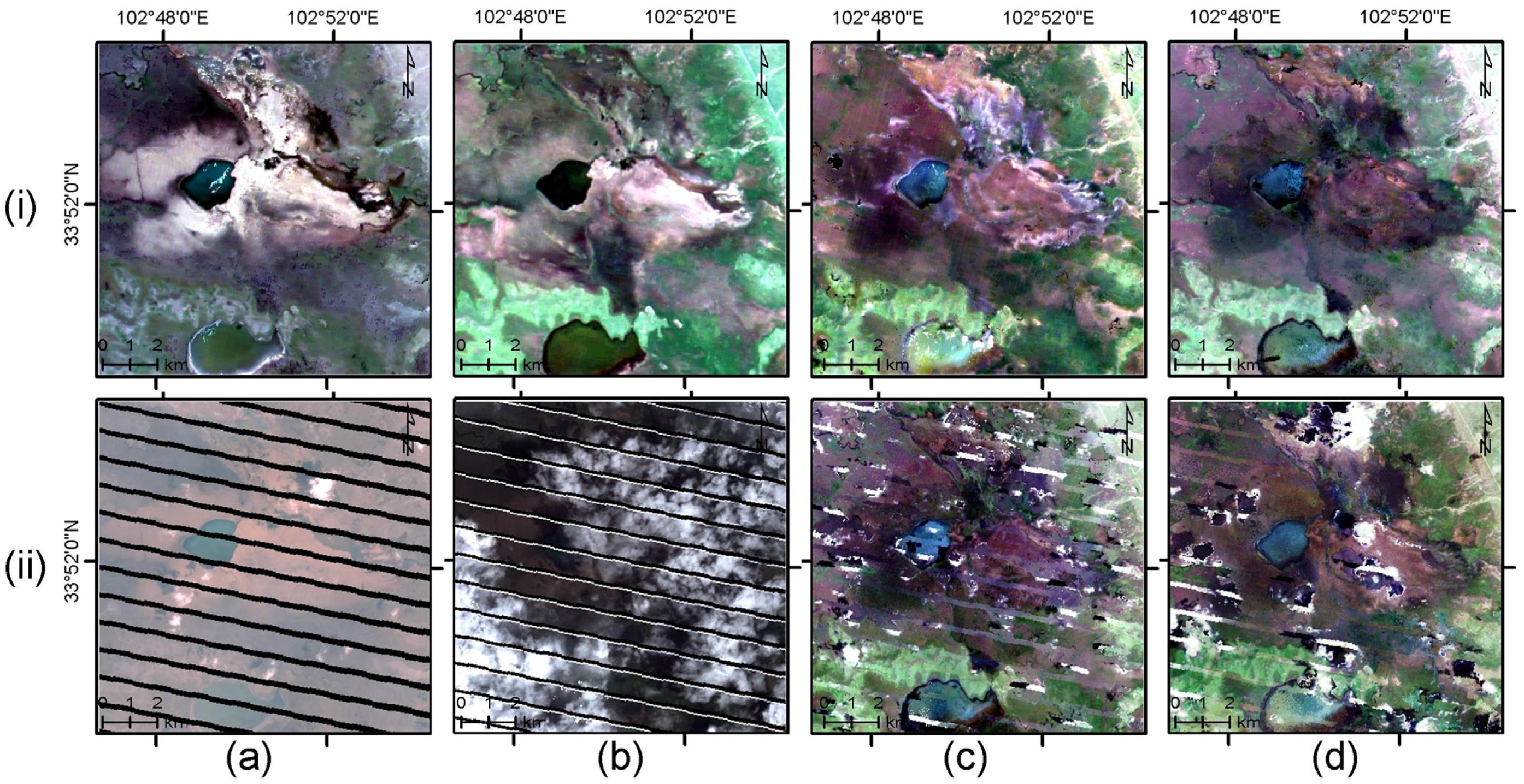
4.1. Performance of the Composites for Reducing Cloud Contamination

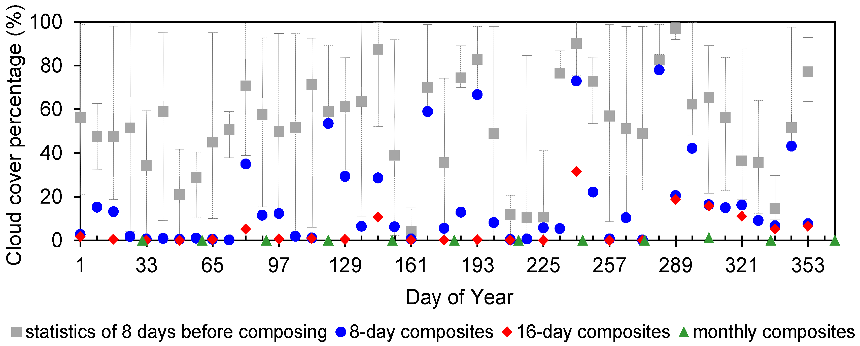
4.1.1. Statistics of the Cloud Cover Percentage

The 8-day, 16-day and monthly composites were generated from all the HJ-1A/B imagery in 2010. Figure 4 shows the statistics of the mean cloud cover percentage before and after the composition. The grey blocks with the grey bar were the average cloud cover percentage and its maximum and minimum value in the 8-day compositing period. The blue rounds, red diamonds and green triangle points were the residual cloud cover percentage of the 8-day, 16-day and monthly composites, respectively.

In general, the residual cloud cover percentages of 8-day, 16-day and monthly composites were significantly reduced. Before the temporal composition, the mean cloud cover percentage in 8 days was 46.25%, and the standard deviation (SD) was 33.41%. The 8-day composites yielded substantially lower residual cloud cover percentage than that of original images, with the mean value of 16.37%, and SD of 21.63%. The mean cloud cover percentage for 16-day composites was further decreased to 4.79%, and the SD was decreased to 8.24%, which meant that the 16-day composites were taken almost under clear-sky conditions. The monthly composites were totally cloud free. The lower cloud cover of composites when compared with origin images was expected, because temporal composition can integrate multi-temporal information by compositing a time-series of cloudy images into a representative n-day cloudless image. This is consistent with many previous studies [11,15,19].

Figure 4. Comparison of cloud cover percentage before and after the temporal composition. The grey blocks with the grey bar were the average cloud cover percentage and its maximum and minimum value in the 8-day compositing period. The blue rounds, red diamonds and green triangle points were the residual cloud cover percentage of the 8-day, 16-day and monthly composites, respectively.

Figure 4. Comparison of cloud cover percentage before and after the temporal composition. The grey blocks with the grey bar were the average cloud cover percentage and its maximum and minimum value in the 8-day compositing period. The blue rounds, red diamonds and green triangle points were the residual cloud cover percentage of the 8-day, 16-day and monthly composites, respectively.

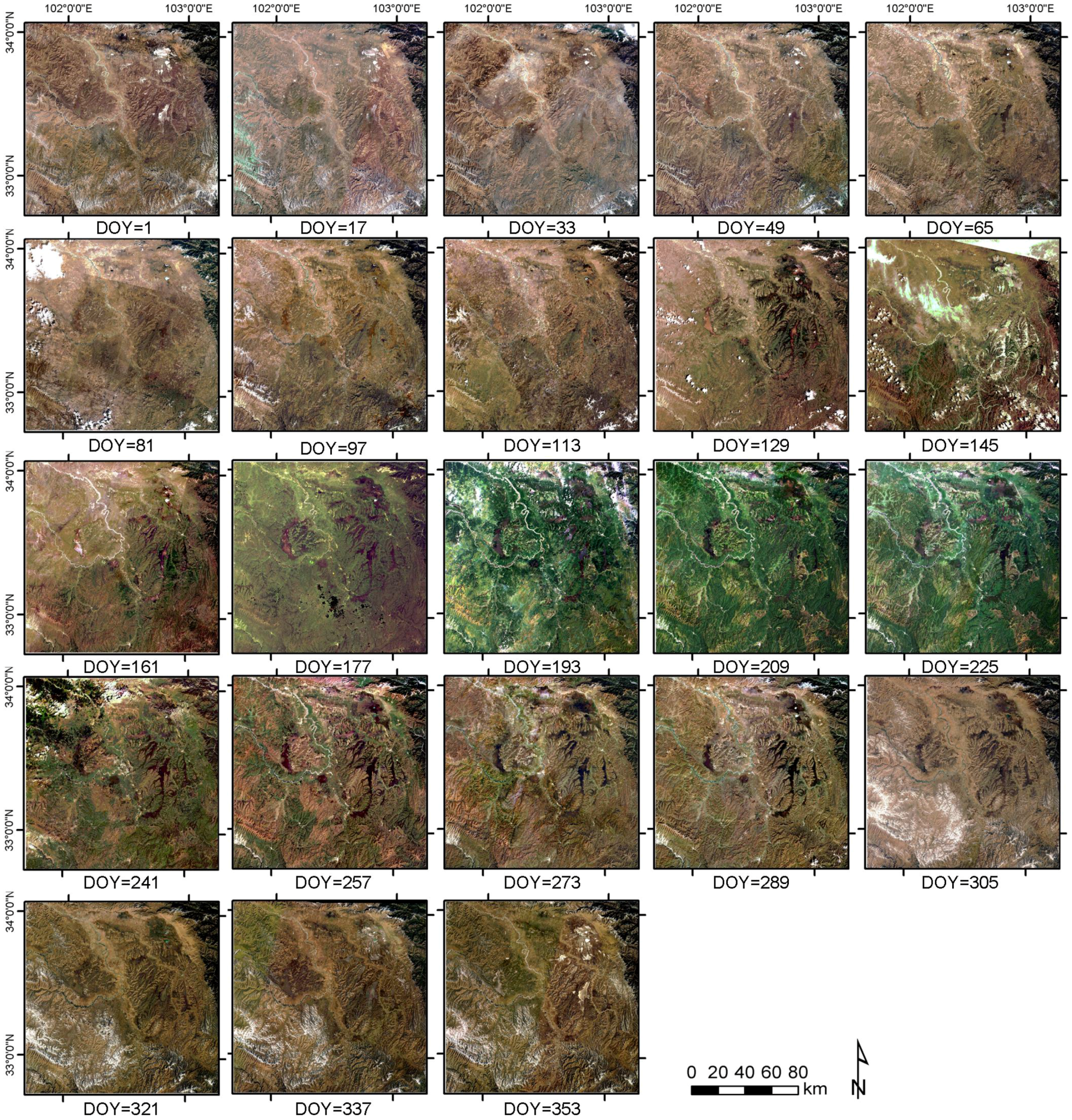
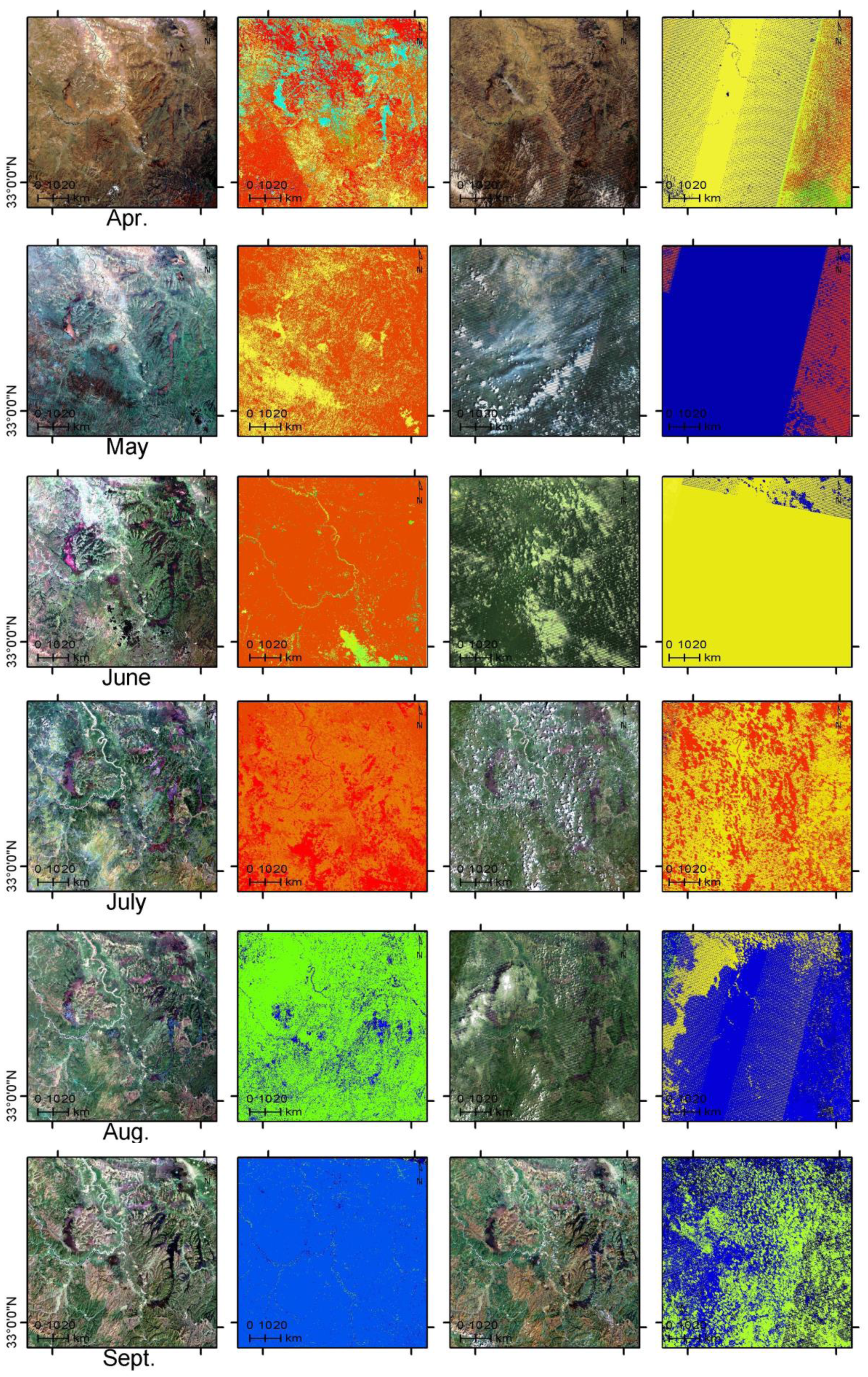
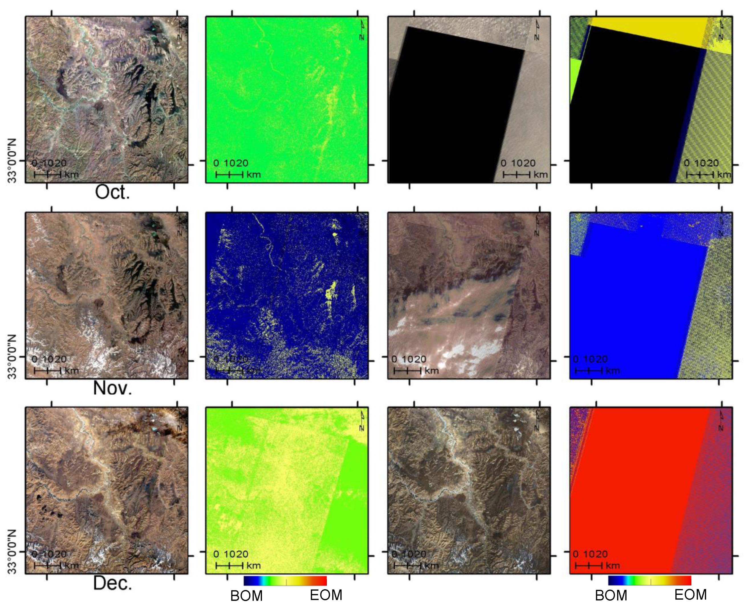
4.1.2. Visual Assessment of 8-Day, 16-Day and Monthly Composites

Figure 5 illustrates the true color browse images that employed red (as red color), green (as green color) and blue (as blue color) band for the 23 scenes of 16-day HJ-1A/B composites. The browse images for 8-day composites and monthly composites are listed in Figure 6 and Figure S1, respectively.

Obviously, the 16-day composites had few clouds. Land covers such as open water, swamps, peat land, and meadow can be accurately retrieved as their outlines were clearly seen in composites for most dates. Also, the spatial distribution and growth process of vegetation can be evidently elucidated from the composites. The green color in the true color composite image normally represents land surface covered by vegetation. As shown in Figure 5, seasonal variations in the greenness of vegetation were evident, with differences in the timing of growth among swamp meadow, meadow and grassland. Besides, the variation trends of wetland inundation, particularly in and around the peat land or open water area were also apparent, where the changes of surface water level were responsible for the combined reflectance effects of mixed pixels. The seasonal variation for vegetation and wetland inundation can be clearly seen in both of the 16-day and 8-day time series composites.

The 8-day composites had relatively more residual clouds than the 16-day composites due to the fewer acquisitions for compositing. Nevertheless, it still showed a good performance in reducing the cloud contamination over the study area.

Figure 5. Browse images for the 16-day composited Top Of Atmosphere (TOA) reflectance results shown with bands 3, 2, 1 in red, green and blue. “DOY” means Day Of Year.

Figure 5. Browse images for the 16-day composited Top Of Atmosphere (TOA) reflectance results shown with bands 3, 2, 1 in red, green and blue. “DOY” means Day Of Year.

4.2. Consistency Assessment with WELD Products

4.2.1. Visual Assessment

Figure 6 shows the browse images of HJ and WELD monthly composites (true color composite) and the corresponding DOY flag images. In general, both HJ and WELD composites can capture the phenology change trend of green vegetation, but the HJ composites were visually better than WELD. For HJ, all of the HJ monthly composites were cloud-free, and the transitional regions between observations from different dates seemed homogeneous for each month. For WELD, half of the images of the 12 months were affected by the Scan Line Corrector (SLC)-off missing data or persistent cloud contamination. Particularly, the no data pixels approximately account for 72.17% and 65.21% in February and October, respectively. The cloud cover percentages for some months (from May to August, and November) in WELD were 9.17%, 29.84%, 6.81%, 10.34% and 28.53%, respectively.

Statistics for the total observations considered in the compositing period were made for both HJ and WELD. For HJ composites, more than 67.21% pixels had 10 or more days of observations within the target month, whilst 26.61% pixels had 15 days or more of observations. About 65.14% of pixels were acquired within four days in the composites. For WELD, only 1.51% pixels had clear observations for all 12 months. The span of days between most WELD pixels ranged from seven days to 25 days. Particularly, about 25.14% of WELD pixels were acquired over more than 15 days.

Figure 6. The visual consistency evaluation (from left to right): (column 1) browse images of HJ-1A/B composites (true color); (column 2) HJ corresponding DOY flag images; (column 3) browse images of Landsat Web-Enabled Landsat Data (WELD) composites (true color); (column 4) WELD corresponding DOY flag images. The black color in February and October in WELD represents no data pixels. “BOM” means beginning of month, and EOM means end of month.

Figure 6. The visual consistency evaluation (from left to right): (column 1) browse images of HJ-1A/B composites (true color); (column 2) HJ corresponding DOY flag images; (column 3) browse images of Landsat Web-Enabled Landsat Data (WELD) composites (true color); (column 4) WELD corresponding DOY flag images. The black color in February and October in WELD represents no data pixels. “BOM” means beginning of month, and EOM means end of month.

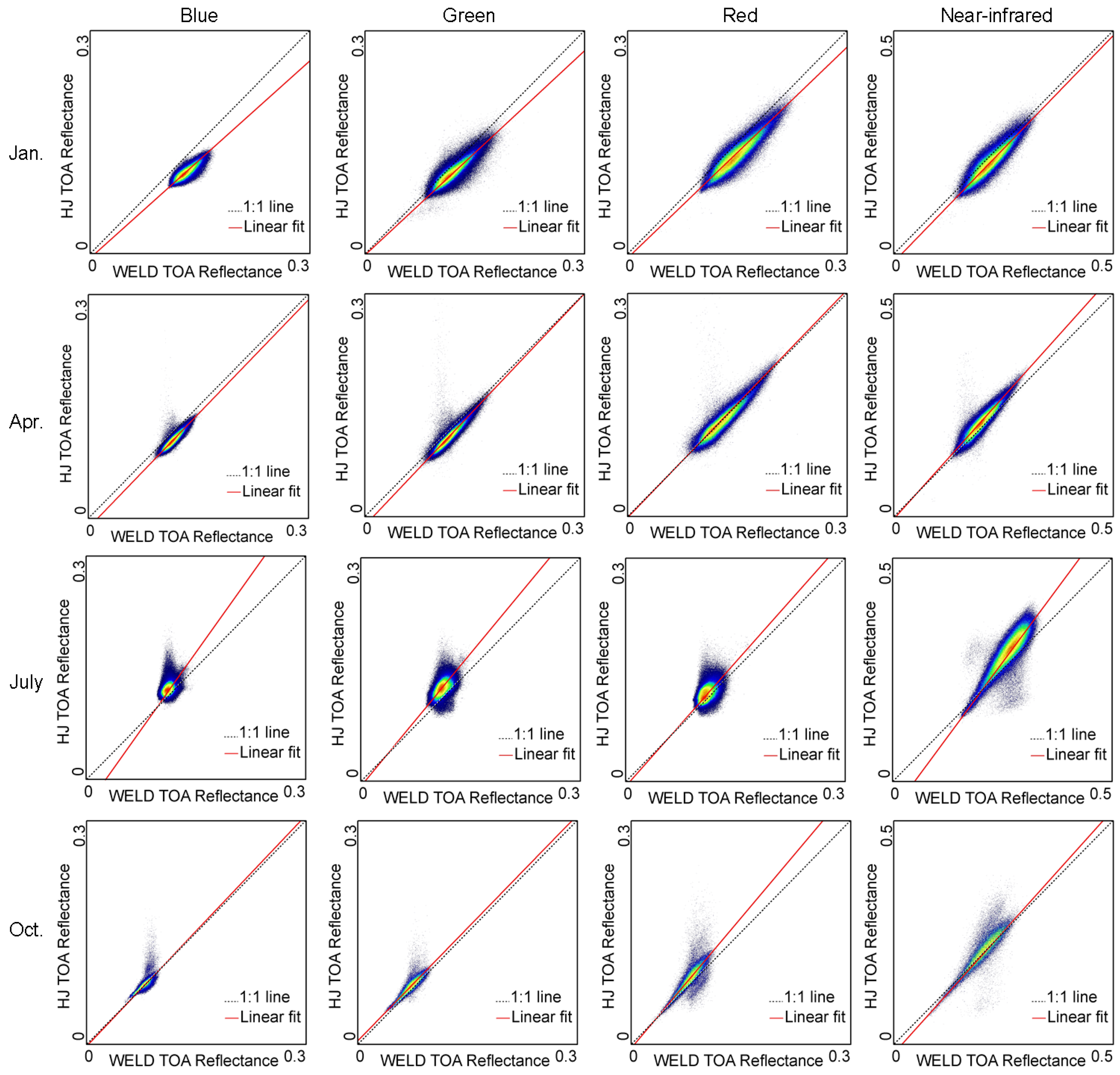
4.2.2. Radiometric Consistency Assessment

To test the radiometric consistency between HJ and WELD, scatterplots of all four bands were drawn for each month. Considering the limitations on space, Figure 7 shows the scatter plots for each middle month of the four seasons. The standard seasonal definition for the Northern Hemisphere adopted by the climate modeling community was used where spring is defined as the months from March to May. The agreement measures for each month are shown in Table 2. Generally, the range of TOA reflectance increased with the growth of vegetation and decreased after the exuberant growing season period. Correlations between TOA reflectance of HJ-1A/B composites and the WELD TOA reflectance were strong in most of the months, with the mean R² ranging from 0.4239–0.6934. The mean slope of linear models ranges from 0.9793–1.1433, with mean intercepts ranging from −0.0159–0.0018. It can be seen from Figure 7 that the visible bands generally exhibited lower consistency than the NIR bands, attributed to the fact that atmospheric effects were inversely proportional to the wavelength.

Correlations between HJ and WELD TOA reflectance were apparently linear in eight months (January to April and September to December) in Table 2. The ranges of R² in these months for each band were 0.4105–0.7040 (blue band), 0.5373–0.7951 (green band), 0.6724–0.8254 (red band) and 0.6933–0.8385 (NIR band), respectively, with mean R² ranging from 0.6695–0.7716. Radiometric consistencies were higher in the near infrared band and lower in the visible wavelengths in these months. For NIR band, the intercepts of linear models were near zero (mean value was −0.0098 and ranged from −0.0201–0.0027) and the slopes ranged from 1.019–1.281. Radiometric consistency for visible bands between HJ and WELD were similar to those of the NIR band. However, the spread of the points were wider, and the reflectances of most of the blue bands of HJ were lower than that of WELD. The slopes for the blue band ranged from 0.7742–1.1714, and intercepts ranged from −0.0185–0.0044, presumably due to more potential clear observations of HJ than WELD.

Figure 7. Scatter plots of WELD TOA reflectance bands (X axis) and HJ TOA reflectance bands (Y axis) for the middle month of every season. The standard seasonal definition for the Northern Hemisphere adopted by the climate modeling community is used where spring is defined by the months March to May. Columns 1–4 are the scatter plots of Blue, Green, Red and Near-infrared bands, respectively. The red solid lines show linear fitted results of the scatter points. The dotted lines are 1:1 lines for reference.

Figure 7. Scatter plots of WELD TOA reflectance bands (X axis) and HJ TOA reflectance bands (Y axis) for the middle month of every season. The standard seasonal definition for the Northern Hemisphere adopted by the climate modeling community is used where spring is defined by the months March to May. Columns 1–4 are the scatter plots of Blue, Green, Red and Near-infrared bands, respectively. The red solid lines show linear fitted results of the scatter points. The dotted lines are 1:1 lines for reference.

Correlations between HJ and WELD were much lower from May to August. Figure 7 showed that the all scatter plots in July deviated from 1:1 line, which indicated there were distinct changes between the two composites. The ranges of R² from May to August for each band were 0.0614–0.2663 (blue band), 0.0931–0.3191 (green band), 0.0593–0.3759 (red band) and 0.2739–0.6977 (NIR band), respectively, with mean R² ranging from 0.1638–0.5369. To further verify the radiometric consistency of the four months with lower R² in Table 2 (i.e., May to August), 400 × 400 pixels subset regions cropped from Figure 6 were shown in Figure 8. Obviously, the composite results of HJ were visually smooth and the color of different land surfaces seemed normal. In contrast, due to there being only two different days available for compositing, still 20.57% and 13.34% of gap pixels stored in WELD in May and June, respectively, were invalid, which was mainly caused by the SLC-off of ETM+ images [47]. Although no invalid pixels appeared in the July and August images, the transition region boundaries were not smooth and many residual cloud patches still remained in the results. The poor atmosphere conditions in the cloudy months are responsible for the discrete distribution of scatter points.

Table 2. Comparison of TOA reflectance for the HJ-1A/B monthly composites and WELD global monthly composite products.

Month	Slope				Intercept				R2				RMSE
	B1	B2	B3	B4	B1	B2	B3	B4	B1	B2	B3	B4	B1	B2	B3	B4
January	0.9329	0.9263	0.9274	1.0190	−0.0128	−0.0012	−0.0039	−0.0104	0.6956	0.7951	0.8173	0.8068	0.0227	0.0134	0.0196	0.0228
February	0.9595	0.9867	0.9503	1.0531	−0.0001	0.0031	0.0059	0.0027	0.4972	0.6330	0.7267	0.7821	0.0114	0.0097	0.0113	0.0166
March	1.0314	1.0180	1.0737	1.1457	−0.0185	−0.0126	−0.0184	−0.0190	0.7040	0.7677	0.8254	0.8385	0.0173	0.0130	0.0135	0.0149
April	1.0246	1.0526	1.0289	1.0980	−0.0134	−0.0135	−0.0018	0.0020	0.6168	0.6597	0.6745	0.7904	0.0304	0.0307	0.0309	0.0350
May	0.7735	0.9091	0.8788	1.0722	0.0336	0.0143	0.0195	0.0100	0.2663	0.3191	0.3759	0.4892	0.0179	0.0191	0.0393	0.0313
June	0.6218	0.5322	0.7231	1.1764	0.0323	0.0365	0.0123	−0.0895	0.0614	0.0931	0.0593	0.2739	0.0245	0.0247	0.0462	0.0986
July	1.4133	1.2928	1.1291	1.3420	−0.0199	−0.0093	−0.0004	−0.0182	0.1611	0.2501	0.3141	0.6871	0.0144	0.0185	0.0153	0.0736
August	1.1458	1.2125	0.9821	1.2190	−0.0148	−0.0121	−0.0102	−0.0146	0.1663	0.2453	0.3638	0.6977	0.0130	0.0147	0.0139	0.0554
September	1.1714	1.1486	1.1628	1.2810	−0.0005	0.0042	−0.0005	−0.0181	0.4329	0.6105	0.7026	0.7141	0.0105	0.0167	0.0117	0.0534
October	1.0268	1.0163	1.1754	1.1680	−0.0006	0.0053	−0.0021	−0.0201	0.4105	0.6392	0.6733	0.7433	0.0176	0.0199	0.0239	0.0362
November	0.8766	0.8358	1.0236	1.0781	0.0039	0.0145	−0.0017	−0.0056	0.4983	0.5373	0.6724	0.6993	0.0156	0.0159	0.0182	0.0260
December	0.7742	0.9038	0.9221	1.0665	0.0044	−0.0081	0.0002	−0.0100	0.5759	0.7131	0.7963	0.7984	0.0292	0.0227	0.0175	0.0137
Mean	0.9793	0.9862	0.9981	1.1433	−0.0005	0.0018	−0.0001	−0.0159	0.4239	0.5219	0.5835	0.6934	0.0187	0.0183	0.0218	0.0398

Table 2. Comparison of TOA reflectance for the HJ-1A/B monthly composites and WELD global monthly composite products.

Month	Slope				Intercept				R2				RMSE
	B1	B2	B3	B4	B1	B2	B3	B4	B1	B2	B3	B4	B1	B2	B3	B4
January	0.9329	0.9263	0.9274	1.0190	−0.0128	−0.0012	−0.0039	−0.0104	0.6956	0.7951	0.8173	0.8068	0.0227	0.0134	0.0196	0.0228
February	0.9595	0.9867	0.9503	1.0531	−0.0001	0.0031	0.0059	0.0027	0.4972	0.6330	0.7267	0.7821	0.0114	0.0097	0.0113	0.0166
March	1.0314	1.0180	1.0737	1.1457	−0.0185	−0.0126	−0.0184	−0.0190	0.7040	0.7677	0.8254	0.8385	0.0173	0.0130	0.0135	0.0149
April	1.0246	1.0526	1.0289	1.0980	−0.0134	−0.0135	−0.0018	0.0020	0.6168	0.6597	0.6745	0.7904	0.0304	0.0307	0.0309	0.0350
May	0.7735	0.9091	0.8788	1.0722	0.0336	0.0143	0.0195	0.0100	0.2663	0.3191	0.3759	0.4892	0.0179	0.0191	0.0393	0.0313
June	0.6218	0.5322	0.7231	1.1764	0.0323	0.0365	0.0123	−0.0895	0.0614	0.0931	0.0593	0.2739	0.0245	0.0247	0.0462	0.0986
July	1.4133	1.2928	1.1291	1.3420	−0.0199	−0.0093	−0.0004	−0.0182	0.1611	0.2501	0.3141	0.6871	0.0144	0.0185	0.0153	0.0736
August	1.1458	1.2125	0.9821	1.2190	−0.0148	−0.0121	−0.0102	−0.0146	0.1663	0.2453	0.3638	0.6977	0.0130	0.0147	0.0139	0.0554
September	1.1714	1.1486	1.1628	1.2810	−0.0005	0.0042	−0.0005	−0.0181	0.4329	0.6105	0.7026	0.7141	0.0105	0.0167	0.0117	0.0534
October	1.0268	1.0163	1.1754	1.1680	−0.0006	0.0053	−0.0021	−0.0201	0.4105	0.6392	0.6733	0.7433	0.0176	0.0199	0.0239	0.0362
November	0.8766	0.8358	1.0236	1.0781	0.0039	0.0145	−0.0017	−0.0056	0.4983	0.5373	0.6724	0.6993	0.0156	0.0159	0.0182	0.0260
December	0.7742	0.9038	0.9221	1.0665	0.0044	−0.0081	0.0002	−0.0100	0.5759	0.7131	0.7963	0.7984	0.0292	0.0227	0.0175	0.0137
Mean	0.9793	0.9862	0.9981	1.1433	−0.0005	0.0018	−0.0001	−0.0159	0.4239	0.5219	0.5835	0.6934	0.0187	0.0183	0.0218	0.0398

Figure 8. Monthly composited detailed regions of HJ (row (i)) and WELD (row (ii)) cropped from Figure 6. (a–d) are the enlarged details from May, June, July and August, respectively.

Figure 8. Monthly composited detailed regions of HJ (row (i)) and WELD (row (ii)) cropped from Figure 6. (a–d) are the enlarged details from May, June, July and August, respectively.

4.2.3. Temporal Profile

To further check the temporal coherence of the composites, Figure 9a–f shows the NDVI profiles of the six typical land covers, namely the sand land, open water, residential land, peat land, grassland and coniferous forest in Zoige plateau, for comparison. These six typical land covers represented different surface phenology and complexity. The NDVI profiles were retrieved from the corresponding regions cropped from Figure 7. To enhance visual judgment, the corresponding ground photos were shown to reflect the actual ground vegetation types.

On the whole, the general change patterns of NDVI profiles were apparent from both products. The HJ NDVI and WELD NDVI profiles were in good agreement for most of the land cover types. For example, the profiles for sand land, residential land and open water were very close. This good agreement indicated that the HJ composites had a similar monitoring capability to the WELD products. Of the two products, the WELD obtained the lower NDVI value for most periods of the six land covers. Such low values were more obvious for land cover like peat land, grassland and needle-leaf forest when the growth season began. These low WELD NDVI values can be explained by the fact that the compositing methods depended on the density of observations. In addition, a gap was found in the WELD open water NDVI profile. This was caused by the lack of valid observations in the corresponding month (Figure 6). A sudden fall that does not conform to the trend of vegetation growth that can be seen in the WELD grassland profile. This was most likely caused by cloud contamination. In short, these results suggested that the HJ composites provided a comparably high quality temporal profile and showed a better performance for the time series analysis of different land cover types.

Figure 9. Monthly mean TOA NDVI profiles of six typical land covers (a–f) and their standard deviation values at corresponding window locations extracted from the monthly HJ and WELD composites. The six ground photos show the actual ground land cover types for each NDVI temporal profile.

Figure 9. Monthly mean TOA NDVI profiles of six typical land covers (a–f) and their standard deviation values at corresponding window locations extracted from the monthly HJ and WELD composites. The six ground photos show the actual ground land cover types for each NDVI temporal profile.

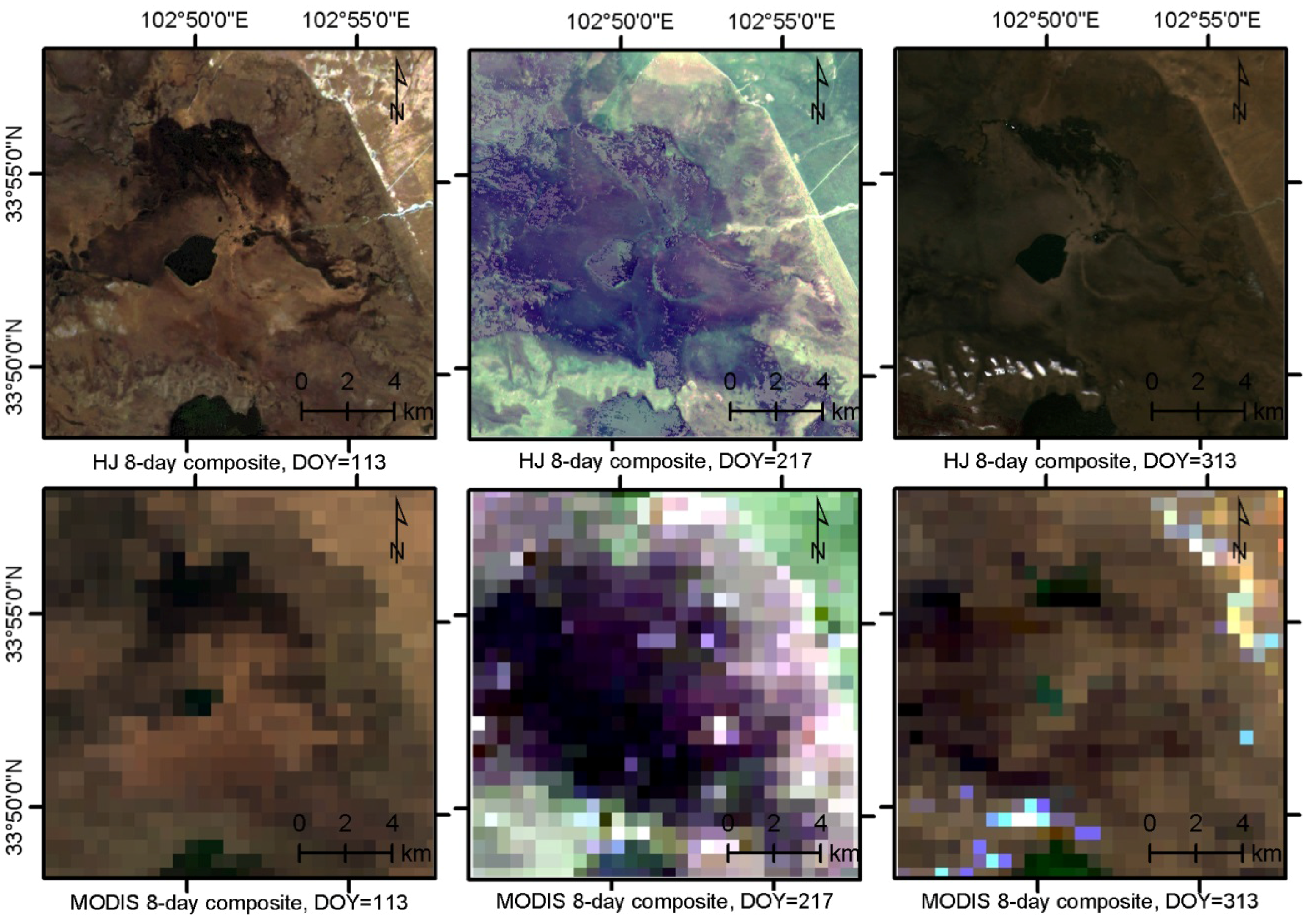
4.3. Consistency Assessment with MODIS Products

4.3.1. Comparison with 8-Day MODIS Reflectance Product

Figure 10 shows partially enlarged details (true color) of 8-day HJ-1A/B TOA reflectance (the upper row) and MODIS MOD09A1 (the lower row) for three different dates, representing the early stage (DOY 113), the vigorous stage (DOY 217) and the end stage (DOY 313) of the growth season respectively [30]. The MODIS images were produced with an RGB color scheme that employs bands B1 (as red color), B4 (as green color) and B3 (as blue color).

Figure 10. Comparison between the enlarged details of 8-day composited HJ-1A/B TOA reflectance (upper) and the 8-day MODIS MOD09A1 surface reflectance product (lower). The HJ-1A/B composites are shown with bands 3, 2, 1 and the MODIS MOD09A1 are shown with bands 1, 4, 3 in red, green and blue.

Figure 10. Comparison between the enlarged details of 8-day composited HJ-1A/B TOA reflectance (upper) and the 8-day MODIS MOD09A1 surface reflectance product (lower). The HJ-1A/B composites are shown with bands 3, 2, 1 and the MODIS MOD09A1 are shown with bands 1, 4, 3 in red, green and blue.

Overall, a higher visual quality was evident from the upper row images which more clearly illustrated the spatial details of different land covers in Zoige plateau wetland. As MOD09 contains mostly mixed pixels, it cannot reveal the inner differences of the wetland areas. The difference of spectral reflectance for grasslands was regarded as slight in the early and end stages of the growth season [48], and therefore the background information of soil usually dominated in the coarse pixels during these periods. Obviously, the slight difference of grasslands can be clearly distinguished from HJ composites in DOY 113. On the other hand, MOD09 can only delineate the boundaries of some main types of land cover, such as the water body, peat land, and grassland. The complexity of wetland land surfaces was the highest during the vigorous stage in the three stages due to the seasonal inundation and the vigorous growth of vegetation. In this stage, most of the helobious grassland and hygrophilous grassland pixels were mixtures of grass, peat land or water. The characteristics of wetland in the vigorous stage can be clearly indicated in the HJ composition imagery (DOY 217). The MOD09 product has some shortage relative to HJ due to the interaction of coarser pixel size with landscape distribution characteristics leading to loss of spatial information. For example, the lake boundary, which can be clearly recognized in DOY 113 and DOY 313, was mixed with the peat land in DOY 217. At the end stage of the growth season, HJ can still discriminate the spatial characteristics of the wetland landscape.

4.3.2. Comparison with 16-Day MODIS NDVI Product

Figure 11 shows a scatter plot of all the comparable samples selected from the HJ 16-day composited NDVI and the 16-day MODIS NDVI products. Overall, the samples were generally distributed around the 1:1 line, and good agreement was found between the HJ-1A/B NDVI and the MODIS NDVI, with the R² reaching 0.9312. In addition, the correlation was strongly linear, and the slope of the regression line was close to 1. The good agreement between the HJ-1A/B NDVI and the well-verified MODIS NDVI product suggested that the overall quality of HJ-1A/B NDVI was high. However, there is a systematic bias that the MODIS NDVI is on average 0.067 greater than HJ TOA NDVI. Such systematic bias can be partly explained by the fact that the MODIS NDVI product is derived from atmospherically corrected data while the HJ TOA NDVI is calculated from TOA reflectance. Similar results had been found in the comparison between surface and TOA NDVI of WELD done by Roy et al. [49], which demonstrated that surface NDVI was on average 0.1 greater than the TOA NDVI for “vegetated” surface. In addition, the systematic bias may also include an effect from the different sensor’s Spectral Response Function (SRF) between HJ and MODIS (Figure 2). Previous studies pointed out that NDVI is sensitive to the sensor’s SRF, and the difference of the SRF should be considered for the comparison between different sensors [50,51].

Figure 11. Scatter plot for the comparable samples in the year 2010 with HJ-1A/B 16-day composited TOA-NDVI as x-axis and MODIS 16-day NDVI (MOD13A1) as y-axis.

Figure 11. Scatter plot for the comparable samples in the year 2010 with HJ-1A/B 16-day composited TOA-NDVI as x-axis and MODIS 16-day NDVI (MOD13A1) as y-axis.

5. Discussion

Fine spatio-temporal resolution images can typically provide detailed land surface dynamics which the coarse spatial resolution images cannot supply. Generating the consistent and comparative fine spatio-temporal imagery product is therefore critical for deepening understanding of earth surface processes. Image compositing techniques that select the most suitable pixel from multi-temporal image acquisitions offer great potential to generate such kinds of products. This paper describes new dense time series products formed by compositing the HJ-1A/B observations. While there have been some studies exploring the use of Landsat TM/ETM+ images for generating the time series products on a 30-m spatial scale [11,15,19,21], the proposed composited product in this paper reflected that a higher temporal resolution composited product can be obtained by using 2-day repeat coverage data. The compositing approach includes some key issues that are worth attention.

The compositing approach took advantage of the automatic pre-processing methods for geometric registration and cloud masking [26]. These methods substantially improved the feasibility of producing HJ-1A/B composites (8-day, 16-day and monthly). The pre-processing methods can easily be implemented on a parallel processor. Nevertheless, since there were some error sources in the pre-processing procedures, a fully automated processing scheme that can provide processing and updating composites in near-real time is needed in future studies. Besides, the cloud shadow detection is more difficult than detecting cloud. There might be some uncertainties about cloud shadow accuracy because of the lack of a thermal-infrared band of HJ-1A/B to determine the cloud height [52]. Although the CV-MVC method is helpful to exclude cloud shadow to some extent, the undetected cloud shadow might be a source of error for the composites.

In this study, the CV-MVC method was used to select the optimum vegetation pixel from available observations. However, for the none-vegetation pixels such as water, peat lands or sand lands, the NDVI profile of these pixels do not demonstrate obvious phenology variation trends. Therefore, as shown in Figure 6, the DOY of these none-vegetation areas showed a different trend compared with vegetation pixels in both HJ and WELD. Besides, The CV-MVC method was helpful to exclude some undetected optically thick clouds over vegetation areas. However, for the thin cirrus cloud contaminated areas, the rejection of cloud pixels for the compositing method might not work well because NDVI is less sensitive to those thin cirrus clouds [53]. Besides, since the real earth surface is non-Lambertian, the anisotropy of surface reflectance is an important attribute in satellite observations [13]. The CV-MVC method was also helpful to minimize the bi-directional reflectance effects (BRDF) to some extent [42]. Generally, normalizing the directional reflectance to their nadir-equivalent band reflectance values can increase the radiometric consistency of different dates and lead to the sufficient use of all valid observations [15]. However, in the case of image composition with fine or high spatial resolution, it was not practical to carry out directional reflectance normalization because of the relatively long revisit frequency or narrow FOV. In future studies, the BRDF normalization will be further considered in the HJ composites. BRDF calibration using multi-source ancillary information (such as BRDF parameters from MODIS products) [54,55,56] or deriving BRDF parameters from monthly HJ-1A/B images may be a feasible development.

Two undesired results concerning the residual clouds and the unsmooth transition should be noted in the composites. For the residual clouds, those pixels were mainly dependent on the available valid observations. If no valid observation occurred in the time window for compositing, residual clouds will be included in the results. The other undesired result was the unsmooth transition in the composites. The unsmooth transitions were mainly derived from the variation of atmosphere conditions ion different dates in the compositing period. As the TOA reflectance rather than surface reflectance was used in the current study, the atmosphere condition that contributed differently to the surface reflectance was the main source of error that will introduce bias to the composites. The high accuracy atmosphere correction can be used to further improve the radiometric consistency of the proposed composites [15,49]. However, due to the lack of a shortwave infrared band which was usually needed for aerosol optical depth estimation using the dense dark vegetation approach, the atmosphere correction method for HJ-1A/B imagery is still in the exploratory stage [23,24,34,57]. Atmosphere correction using MODIS atmospheric parameters as the auxiliary data would be helpful for the quality improvement HJ-1A/B composites. In future, the atmosphere corrected surface reflectance will be conducted in the research.

The radiometric calibration error is another important error source that will influence the accuracy of compositing. Some studies have evaluated the radiometric performance of HJ using well-verified TM images or MODIS datasets [58,59], and the results indicated that the image quality of HJ-1A/B CCDs was stable and possessed good consistency. A recent study monitored the radiometric responses of the HJ-1A/B CCD using all available HJ-1A/B images over the pseudo-invariant Dunhuang gobi calibration ground site from 2008–2013 [60]. It indicated that the degradation occurred for all bands of the sensors at different rates and levels. The degradation of sensors might be an important error source which influences the distribution of points in Figure 7. Therefore, a more symmetrically radiometric calibration accuracy evaluation should be performed to provide a more reliable and quantitative radiometric performance knowledge of HJ CCD sensors.

The dense in time series and fine spatial resolution composites can play a key role in providing spatially and temporally explicit data for land surface dynamics monitoring as well as bio-physical parameter retrieving. With the efforts being put into compositing monthly, seasonal or annual imagery products, a broader range of applications have been conducted using these composites [11,20,21,61,62]. Typically, for some more time-sensitive applications such as monitoring rapid disturbance (e.g., insect defoliation, fire, wetland inundation), a smaller composting time window was required. Currently, the capacity of fine spatial resolution images to generate products for such applications is still limited by the satellite revisit frequency [11,21]. Fortunately, opportunities from new satellite missions or virtual constellations will address these limitations. In the future research, dense temporal and high spatial resolution imagery provided by small constellations is a likely possibility for the earth observation satellites [63,64]. With new satellite missions such as Sentinel-2A/B or Landsat 8 Operational Land Imager (OLI) execution [65,66,67], more constellations or virtual constellations would be developed and the integrated measures from different satellite programs will make the temporal repeat frequencies much denser than present. Take the Sentinel-2 for instance. Similar to HJ-1A/B, the Sentinel-2 mission is also based on a pair of satellites configuration (Sentinel-2A and 2B) and has a relatively large swath, allowing a two to three-day revisit time at mid-latitudes. A virtual constellation of HJ-1A/B, Landsat-8 with Sentinel-2 would increase the observation frequency considerably. Such dense data will be particularly beneficial for many time-sensitive application studies [68]. The challenges faced in the work presented here, including differences in bandwidth, location of bands, orbital considerations, and data sharing policy etc. are common to any compositing of virtual constellations. The proposed method can therefore also be used as a reference for generating higher density image products in these situations.

Because the HJ-1A/B imagery can be freely accessed and still runs well on the orbit, the composited methodology can be used to generate HJ composited products for increasingly more areas in the foreseeable future. Particularly, another two small optical satellites will be launched in the “4 + 4” (four optical satellites and four synthetic aperture radar satellites) constellation in the second HJ constellation construction procedure [25]. This paper is a case study to demonstrate the feasibility and potential of using the 30 m HJ-1A/B constellation imagery during a 2-day repeat cycle to create time series (i.e., 8 days, 16 days and monthly) 30-m composites which can better reflect the variability of vegetation in heterogeneous regions. The detailed methodology and performance of the results were systemically introduced. The composited method in this paper is general and can be easily implemented for other areas. Efforts in the future will focus on testing the proposed method for large scale areas, and more image process procedures such as radiometric topographic correction should be included to improve the radiometric consistency [56,69].

6. Conclusions

Dense time series and fine spatial resolution remote sensing images (e.g., 30-m) are urgently needed for monitoring detailed land surface dynamics. In this study, new time series 30-m imagery products with 8-day, 16-day and monthly time intervals were generated using the 2-day revisiting HJ-1A/B observations. Building on automated orthorectification and cloud masking algorithms previously developed for HJ data, this study demonstrates the feasibility of using HJ-1A/B images to produce 30-m composites which can reflect the vegetation dynamics in a heterogeneous area over eight days, 16 days and one month.

Quality assessment was performed by comparing the HJ composites with the well-verified WELD and MODIS products. HJ composites have no data gaps and have substantially less cloud contamination than WELD data. Good agreements were found between the monthly WELD and HJ TOA reflectance for eight months (January to April, September to December) with a mean R² for blue, green, red and near-infrared bands of 0.5539, 0.6695, 0.7361, and 0.7716, respectively. An obviously lower R² value was found for the scatter plots in May, June, July and August when more clouds and data gaps appeared in WELD in this period. HJ showed a better temporal coherence than WELD according to the time series analysis of the TOA NDVI profile. The comparison between HJ and MODIS revealed that the HJ composites are comparable to MODIS data over areas consisting of large patches of homogeneous surface types, but can provide 30-m spatial details for fragmented landscapes. Mean residual cloud cover percentage statistics indicated that the mean residual clouds for 8-day, 16-day and monthly HJ composites were 16.37%, 4.79%, and cloud free, respectively. It is believed that the HJ composites are comparably high-quality products in terms of both temporal profile and radiometric consistency.

Generally, the compositing efforts conducted in this study illustrate that the compositing of HJ-1A/B observations can provide datasets at dense temporal resolution and fine spatial resolution, and it overcomes the difficulty of less clear-sky observations. However, as there are some unsolved problems such as the precise atmospheric correction and BRDF normalization for HJ-1A/B images, the methodology only partially exploited the temporal information by using the TOA reflectance measures. More explicit utilization of the consistent surface reflectance will further enhance the quality of composited products.

References

1. Justice, C.O.; Vermote, E.; Townshend, J.R.G.; Defries, R.; Roy, D.P.; Hall, D.K.; Salomonson, V.V.; Privette, J.L.; Riggs, G.; Strahler, A.; et al. The moderate resolution imaging spectroradiometer (MODIS): Land remote sensing for global change research. IEEE Trans. Geosci. Remote Sens. 1998, 36, 1228–1249. [Google Scholar] [CrossRef]
2. Tanre, D.; Holben, B.N.; Kaufman, Y.J. Atmospheric correction against algorithm for NOAA-AVHRR products: Theory and application. IEEE Trans. Geosci. Remote Sens. 1992, 30, 231–248. [Google Scholar] [CrossRef]
3. Zhao, W.; Li, A.; Bian, J.; Jin, H.; Zhang, Z. A synergetic algorithm for mid-morning land surface soil and vegetation temperatures estimation using MSG-SEVIRI products and TERRA-MODIS products. Remote Sens. 2014, 6, 2213–2238. [Google Scholar] [CrossRef]
4. Zhu, X.; Chen, J.; Gao, F.; Chen, X.; Masek, J.G. An enhanced spatial and temporal adaptive reflectance fusion model for complex heterogeneous regions. Remote Sens Environ. 2010, 114, 2610–2623. [Google Scholar] [CrossRef]
5. Huang, C.Q.; Coward, S.N.; Masek, J.G.; Thomas, N.; Zhu, Z.L.; Vogelmann, J.E. An automated approach for reconstructing recent forest disturbance history using dense Landsat time series stacks. Remote Sens. Environ. 2010, 114, 183–198. [Google Scholar] [CrossRef]
6. Li, A.; Huang, C.; Sun, G.; Shi, H.; Toney, C.; Zhu, Z.L.; Rollins, M.; Goward, S.; Masek, J. Modeling the height of young forests regenerating from recent disturbances in Mississippi using Landsat and ICESat data. Remote Sens. Environ. 2011, 115, 1837–1849. [Google Scholar] [CrossRef]
7. Sexton, J.O.; Song, X.-P.; Feng, M.; Noojipady, P.; Anand, A.; Huang, C.; Kim, D.-H.; Collins, K.M.; Channan, S.; DiMiceli, C. Global, 30-m resolution continuous fields of tree cover: Landsat-based rescaling of MODIS vegetation continuous fields with Lidar-based estimates of error. Int. J. Digit. Earth 2013, 6, 427–448. [Google Scholar] [CrossRef]
8. Lehmann, E.A.; Wallace, J.F.; Caccetta, P.A.; Furby, S.L.; Zdunic, K. Forest cover trends from time series Landsat data for the Australian continent. Int. J. Appl. Earth. Obs. 2013, 21, 453–462. [Google Scholar] [CrossRef]
9. Li, A.; Lei, G.; Zhang, Z.; Bian, J.; Deng, W. China land cover monitoring in mountainous regions by remote sensing technology—Taking the southwestern China as a case. In Proceedings of the 2014 IEEE International Geoscience and Remote Sensing Symposium (IGARSS 2014), Quebec, QC, Canada, 13–18 July 2014; pp. 4216–4219.
10. Townshend, J.R.G.; Justice, C.O. Selecting the spatial-resolution of satellite sensors required for global monitoring of land transformations. Int. J. Remote Sens. 1988, 9, 187–236. [Google Scholar] [CrossRef]
11. White, J.C.; Wulder, M.A.; Hobart, G.W.; Luther, J.E.; Hermosilla, T.; Griffiths, P.; Coops, N.C.; Hall, R.J.; Hostert, P.; Dyk, A.; et al. Pixel-based image compositing for large-area dense time series applications and science. Can. J. Remote Sens. 2014, 40, 192–212. [Google Scholar] [CrossRef]
12. Holben, B.N. Characteristics of maximum-value composite images from temporal AVHRR data. Int. J. Remote Sens. 1986, 7, 1417–1434. [Google Scholar] [CrossRef]
13. Luo, Y.; Trishchenko, A.P.; Khlopenkov, K.V. Developing clear-sky, cloud and cloud shadow mask for producing clear-sky composites at 250-meter spatial resolution for the seven MODIS land bands over Canada and north America. Remote Sens. Environ. 2008, 112, 4167–4185. [Google Scholar] [CrossRef]
14. Shen, H.; Li, X.; Cheng, Q.; Zheng, C.; Yang, G.; Li, H.; Zhang, L. Missing information reconstruction of remote sensing data: A technical review. IEEE Geosci. Remote Sens. Mag. 2015, 3, 61–85. [Google Scholar] [CrossRef]
15. Roy, D.P.; Ju, J.C.; Kline, K.; Scaramuzza, P.L.; Kovalskyy, V.; Hansen, M.; Loveland, T.R.; Vermote, E.; Zhang, C.S. Web-Enabled Landsat Data (WELD): Landsat ETM plus composited mosaics of the conterminous United States. Remote Sens. Environ. 2010, 114, 35–49. [Google Scholar] [CrossRef]
16. Potapov, P.V.; Turubanova, S.A.; Hansen, M.C.; Adusei, B.; Broich, M.; Altstatt, A.; Mane, L.; Justice, C.O. Quantifying forest cover loss in democratic republic of the congo, 2000–2010, with Landsat ETM plus data. Remote Sens. Environ. 2012, 122, 106–116. [Google Scholar] [CrossRef]
17. Flood, N. Seasonal composite Landsat TM/ETM plus images using the medoid (a multi-dimensional median). Remote Sens. 2013, 5, 6481–6500. [Google Scholar] [CrossRef]
18. Kovalskyy, V.; Roy, D.P. The global availability of Landsat 5 TM and Landsat 7 ETM+ land surface observations and implications for global 30m Landsat data product generation. Remote Sens. Environ. 2013, 130, 280–293. [Google Scholar] [CrossRef]
19. Griffiths, P.; van der Linden, S.; Kuemmerle, T.; Hostert, P. Pixel-based Landsat compositing algorithm for large area land cover mapping. IEEE J-STARS 2013, 6, 2088–2101. [Google Scholar] [CrossRef]
20. Yan, L.; Roy, D. Automated crop field extraction from multi-temporal web enabled Landsat data. Remote Sens. Environ. 2014, 144, 42–64. [Google Scholar] [CrossRef]
21. Hansen, M.C.; Egorov, A.; Potapov, P.V.; Stehman, S.V.; Tyukavina, A.; Turubanova, S.A.; Roy, D.P.; Goetz, S.J.; Loveland, T.R.; Ju, J.; et al. Monitoring conterminous United States (CONUS) land cover change with web-enabled Landsat data (WELD). Remote Sens. Environ. 2014, 140, 466–484. [Google Scholar] [CrossRef]
22. Yan, L.; Roy, D.P. Improved time series land cover classification by missing-observation-adaptive nonlinear dimensionality reduction. Remote Sens. Environ. 2015, 158, 478–491. [Google Scholar] [CrossRef]
23. Sun, L.; Sun, C.; Liu, Q.; Zhong, B. Aerosol optical depth retrieval by HJ-1/CCD supported by MODIS surface reflectance data. Sci. China Earth Sci. 2010, 53, 74–80. [Google Scholar] [CrossRef]
24. Tian, L.; Lu, J.; Chen, X.; Yu, Z.; Xiao, J.; Qiu, F.; Zhao, X. Atmospheric correction of HJ-1A/B CCD images over Chinese coastal waters using MODIS-TERRA aerosol data. Sci. China Technol. Sci. 2010, 53, 191–195. [Google Scholar] [CrossRef]
25. Wang, Q.; Wu, C.; Li, Q.; Li, J. Chinese HJ-1A/B satellites and data characteristics. Sci. China Earth Sci. 2010, 53, 51–57. [Google Scholar] [CrossRef]
26. Bian, J.; Li, A.; Jin, H.; Lei, G.; Huang, C.; Li, M. Auto-registration and orthorectification algorithm for the time series HJ-1A/B CCD images. J. Mt. Sci. 2013, 10, 754–767. [Google Scholar] [CrossRef]
27. Chen, J.; Cui, T.W.; Qiu, Z.F.; Lin, C.S. A three-band semi-analytical model for deriving total suspended sediment concentration from HJ-1A/CCD data in turbid coastal waters. ISPRS J. Photogramm. Remote Sens. 2014, 93, 1–13. [Google Scholar] [CrossRef]
28. Bian, J.; Li, A.; Jin, H.; Zhao, W.; Lei, G.; Huang, C. Multi-temporal cloud and snow detection algorithm for the HJ-1A/B CCD imagery of China. In Proceedings of the 2014 IEEE International Geoscience and Remote Sensing Symposium (IGARSS 2014), Quebec, QC, Canada, 13–18 July 2014; pp. 501–504.
29. Bian, J.; Li, A.; Deng, W. Estimation and analysis of net primary productivity of Ruoergai wetland in China for the recent 10 years based on remote sensing. Procedia Environ. Sci. 2010, 2, 288–301. [Google Scholar] [CrossRef]
30. Zhao, Y.; Yu, Z.C.; Zhao, W.W. Holocene vegetation and climate histories in the eastern Tibetan plateau: Controls by insolation-driven temperature or monsoon-derived precipitation changes? Quat. Sci. Rev. 2011, 30, 1173–1184. [Google Scholar] [CrossRef]
31. Li, A.; Bian, J.; Lei, G.; Huang, C. Estimating the maximal light use efficiency for different vegetation through CASA model combined with time-series remote sensing data and ground measurements. Remote Sens. 2012, 4, 3857–3876. [Google Scholar] [CrossRef]
32. Lu, S.L.; Wu, B.F.; Yan, N.N.; Wang, H. Water body mapping method with hj-1a/b satellite imagery. Int. J. Earth Obs. 2011, 13, 428–434. [Google Scholar] [CrossRef]
33. China Centre for Resources Satellite Data and Application. Available online: http://www.Cresda.Com/site2/satellite/7117.Shtml (accessed on 1 September 2015).
34. Zhao, Z.; Li, A.; Bian, J.; Huang, C. An improved ddv method to retrieve aot for HJ CCD image in typical mountainous areas. Spectrosc. Spect. Anal. 2015, 35, 1479–1487. (In Chinese) [Google Scholar]
35. Wolfe, R.E.; Nishihama, M.; Fleig, A.J.; Kuyper, J.A.; Roy, D.P.; Storey, J.C.; Patt, F.S. Achieving sub-pixel geolocation accuracy in support of MODIS land science. Remote Sens. Environ. 2002, 83, 31–49. [Google Scholar] [CrossRef]
36. Gutman, G.; Huang, C.Q.; Chander, G.; Noojipady, P.; Masek, J.G. Assessment of the NASA-USGS Global Land Survey (GLS) datasets. Remote Sens. Environ. 2013, 134, 249–265. [Google Scholar] [CrossRef]
37. Bian, J.; Li, A.; Huang, C. Cloud and snow discrimination for CCD images of HJ-1A/B constellation based on spectral signature and spatio-temporal context. Remote Sens. 2015. submitted. [Google Scholar]
38. Gomez-Chova, L.; Camps-Valls, G.; Calpe-Maravilla, J.; Guanter, L.; Moreno, J. Cloud-screening algorithm for envisat/meris multispectral images. IEEE Trans. Geosci. Remote. Sens. 2007, 45, 4105–4118. [Google Scholar] [CrossRef]
39. Zhang, Y.; Guindon, B.; Cihlar, J. An image transform to characterize and compensate for spatial variations in thin cloud contamination of landsat images. Remote Sens. Environ. 2002, 82, 173–187. [Google Scholar] [CrossRef]
40. Friesen, L.J.; Jackson, A.A.; Zook, H.A.; Kessler, D.J. Analysis of orbital perturbations acting on objects in orbits near geosynchronous earth orbit. J. Geophys. Res. Planet 1992, 97, 3845–3863. [Google Scholar] [CrossRef]
41. Liu, L.; Wang, X.; Bai, Z.; Tang, T.; Yu, G. Orbit maintenance technology and implement for HJ-1A/B constellation. Chinese Space Science and Technology 2012, 5, 69–75. (In Chinese) [Google Scholar]
42. Van Leeuwen, W.J.D.; Huete, A.R.; Laing, T.W. MODIS vegetation index compositing approach: A prototype with AVHRR data. Remote Sens. Environ. 1999, 69, 264–280. [Google Scholar] [CrossRef]
43. Walthall, C.L.; Norman, J.M.; Welles, J.M.; Campbell, G.; Blad, B.L. Simple equation to approximate the bidirectional reflectance from vegetative canopies and bare soil surfaces. Appl. Opt. 1985, 24, 383–387. [Google Scholar] [CrossRef] [PubMed]
44. USGS National Center for Earth Resources Observation and Science (EROS). Available online: http://globalweld.cr.usgs.gov/ (accessed on 1 September 2015).
45. Kaufman, Y.J.; Tanre, D. Atmospherically Resistant Vegetation Index (ARVI) for EOS-MODIS. IEEE Trans. Geosci. Remote Sens. 1992, 30, 261–270. [Google Scholar] [CrossRef]
46. Feng, M.; Sexton, J.O.; Huang, C.; Masek, J.G.; Vermote, E.F.; Gao, F.; Narasimhan, R.; Channan, S.; Wolfe, R.E.; Townshend, J.R. Global surface reflectance products from Landsat: Assessment using coincident MODIS observations. Remote Sens. Environ. 2013, 134, 276–293. [Google Scholar] [CrossRef]
47. Chen, J.; Zhu, X.L.; Vogelmann, J.E.; Gao, F.; Jin, S.M. A simple and effective method for filling gaps in Landsat ETM plus SLC-off images. Remote Sens. Environ. 2011, 115, 1053–1064. [Google Scholar] [CrossRef]
48. Psomas, A.; Zimmermann, N.E.; Kneubühler, M.; Kellenberger, T.; Itten, A.K. Seasonal variability in spectral reflectance for discriminating grasslands along a dry-mesic gradient in Switzerland. In Proceedings of the 4th EARSEL Workshop on Imaging Spectroscopy, Warsaw, Poland; 2005; pp. 709–722. [Google Scholar]
49. Roy, D.P.; Qin, Y.; Kovalskyy, V.; Vermote, E.F.; Ju, J.; Egorov, A.; Hansen, M.C.; Kommareddy, I.; Yan, L. Conterminous united states demonstration and characterization of MODIS-based Landsat ETM+ atmospheric correction. Remote Sens. Environ. 2014, 140, 433–449. [Google Scholar] [CrossRef]
50. Trishchenko, A.P.; Cihlar, J.; Li, Z.Q. Effects of spectral response function on surface reflectance and NDVI measured with moderate resolution satellite sensors. Remote Sens. Environ. 2002, 81, 1–18. [Google Scholar] [CrossRef]
51. Gonsamo, A.; Chen, J.M. Spectral response function comparability among 21 satellite sensors for vegetation monitoring. IEEE Trans. Geosci. Remote Sens. 2013, 51, 1319–1335. [Google Scholar] [CrossRef]
52. Zhu, Z.; Woodcock, C.E. Object-based cloud and cloud shadow detection in landsat imagery. Remote Sens. Environ. 2012, 118, 83–94. [Google Scholar] [CrossRef]
53. Hagolle, O.; Lobo, A.; Maisongrande, P.; Cabot, F.; Duchemin, B.; De Pereyra, A. Quality assessment and improvement of temporally composited products of remotely sensed imagery by combination of vegetation 1 and 2 images. Remote Sens. Environ. 2005, 94, 172–186. [Google Scholar] [CrossRef] [Green Version]
54. Li, F.; Jupp, D.L.; Thankappan, M.; Lymburner, L.; Mueller, N.; Lewis, A.; Held, A. A physics-based atmospheric and BRDF correction for Landsat data over mountainous terrain. Remote Sens. Environ. 2012, 124, 756–770. [Google Scholar] [CrossRef]
55. Flood, N. Testing the local applicability of MODIS BRDF parameters for correcting landsat TM imagery. Remote Sens. Lett. 2013, 4, 793–802. [Google Scholar] [CrossRef]
56. Li, A.; Wang, Q.; Bian, J.; Lei, G. An improved physics-based model for topographic correction of Landsat TM images. Remote Sens. 2015, 7, 6296–6319. [Google Scholar] [CrossRef]
57. Zhao, Z.; Li, A.; Bian, J.; Guo, W.; Liu, Q.; Zhao, W.; Huang, C. Automatic detection of the DDV pixels from VIS-NIR images in typical mountainous areas. Remote Sens. Technol. Appl. 2015, 30, 58–67. (In Chinese) [Google Scholar]
58. Jiang, B.; Liang, S.; Townshend, J.R.; Dodson, Z.M. Assessment of the radiometric performance of Chinese HJ-1 satellite ccd instruments. IEEE J-STARS 2013, 6, 840–850. [Google Scholar] [CrossRef]
59. Zhang, X.; Zhao, X.; Liu, G.; Kang, Q.; Wu, D. Radioactive quality evaluation and cross validation of data from the HJ-1A/B satellites’ CCD sensors. Sensors 2013, 13, 8564–8576. [Google Scholar] [CrossRef] [PubMed]
60. Li, J.; Chen, X.; Tian, L.; Feng, L. Tracking radiometric responsivity of optical sensors without on-board calibration systems-case of the Chinese HJ-1A/B CCD sensors. Opt. Express 2015, 23, 1829–1847. [Google Scholar] [CrossRef] [PubMed]
61. Kovalskyy, V.; Roy, D.P.; Zhang, X.; Ju, J.C. The suitability of multi-temporal web-enabled landsat data NDVI for phenological monitoring—A comparison with flux tower and MODIS NDVI. Remote Sens. Lett. 2012, 3, 325–334. [Google Scholar] [CrossRef]
62. Hermosilla, T.; Wulder, M.A.; White, J.C.; Coops, N.C.; Hobart, G.W. Regional detection, characterization, and attribution of annual forest change from 1984 to 2012 using Landsat-derived time-series metrics. Remote Sens. Environ. 2015, 170, 121–132. [Google Scholar] [CrossRef]
63. Zhou, G.; Baysal, O.; Kauffmann, P. Current status and future tendency of sensors in earth observing satellites. Available online: http://citeseerx.ist.psu.edu/viewdoc/download?doi=10.1.1.222.3589&rep=rep1&type=pdf (accessed on 1 September 2015).
64. Sandau, R. Status and trends of small satellite missions for earth observation. Acta Astronaut. 2010, 66, 1–12. [Google Scholar] [CrossRef]
65. Drusch, M.; Del Bello, U.; Carlier, S.; Colin, O.; Fernandez, V.; Gascon, F.; Hoersch, B.; Isola, C.; Laberinti, P.; Martimort, P.; et al. Sentinel-2: ESA’s optical high-resolution mission for GMES operational services. Remote Sens. Environ. 2012, 120, 25–36. [Google Scholar] [CrossRef]
66. Roy, D.P.; Wulder, M.A.; Loveland, T.R.; Woodcock, C.E.; Allen, R.G.; Anderson, M.C.; Helder, D.; Irons, J.R.; Johnson, D.M.; Kennedy, R.; et al. Landsat-8: Science and product vision for terrestrial global change research. Remote Sens. Environ. 2014, 145, 154–172. [Google Scholar] [CrossRef]
67. Kovalskyy, V.; Roy, D. A one year Landsat 8 conterminous United States study of cirrus and non-cirrus clouds. Remote Sens. 2015, 7, 564–578. [Google Scholar] [CrossRef]
68. Wulder, M.A.; Hilker, T.; White, J.C.; Coops, N.C.; Masek, J.G.; Pflugmacher, D.; Crevier, Y. Virtual constellations for global terrestrial monitoring. Remote Sens. Environ. 2015, 170, 62–76. [Google Scholar] [CrossRef]
69. Vanonckelen, S.; Lhermitte, S.; Van Rompaey, A. The effect of atmospheric and topographic correction on pixel-based image composites: Improved forest cover detection in mountain environments. Int. J. Appl. Earth Obs. 2015, 35, 320–328. [Google Scholar] [CrossRef]