Superpixel-Based Roughness Measure for Multispectral Satellite Image Segmentation

Abstract

The new generation of artificial satellites is providing a huge amount of Earth observation images whose exploitation can report invaluable benefits, both economical and environmental. However, only a small fraction of this data volume has been analyzed, mainly due to the large human resources needed for that task. In this sense, the development of unsupervised methodologies for the analysis of these images is a priority. In this work, a new unsupervised segmentation algorithm for satellite images is proposed. This algorithm is based on the rough-set theory, and it is inspired by a previous segmentation algorithm defined in the RGB color domain. The main contributions of the new algorithm are: (i) extending the original algorithm to four spectral bands; (ii) the concept of the superpixel is used in order to define the neighborhood similarity of a pixel adapted to the local characteristics of each image; (iii) and two new region merged strategies are proposed and evaluated in order to establish the final number of regions in the segmented image. The experimental results show that the proposed approach improves the results provided by the original method when both are applied to satellite images with different spectral and spatial resolutions.

1. Introduction

Image segmentation is a basic, important step in high level image understanding. It serves as a bridge for the semantic gap between low level image processing and high level image analysis. Segmentation is an integral part in many applications, such as object recognition and tracking [1], land cover and land use classification [2], etc. Image segmentation and specifically multispectral image segmentation is a complex, deeply-studied problem. There is a big corpus of research addressing this problem, but no single algorithm can be considered adequate for all images [3].

A segmentation can be defined as the process of partitioning an image into different non-overlapping homogeneous regions. Usually, segmentation methods are divided into four groups: edge-based, neighborhood-based, histogram-based and cluster-based methods [4].

Edge and neighborhood algorithm-based methods work on the spatial domain of the image. Edge-based algorithms search object contours using the discontinuity property, whereas neighborhood-based algorithms group pixels using a defined similarity property as the homogeneity criteria. Adapting edge-based algorithms to a multispectral domain is not straightforward, so hybrid edge/neighborhood approaches as the ones presented in [5] are common.

Histogram-based and cluster-based segmentation methods operate in the spectral domain of the image. They assume a correspondence between homogeneous image regions and clusters in the spectral representation of the image. Histogram-based algorithms are usually related to the concept of multi-thresholding [6,7,8]. Cluster-based segmentation methods define a heterogeneous set of methods based on different procedures to identify distinct structures in the spectral feature space. Conventional clustering techniques have been successfully applied to satellite image segmentation, such as k-means [9], fuzzy c-means [10] or density-based clustering [11].

The idea of combining spectral and spatial information has also been addressed. This approach usually performs better than methods limited to a unique data domain. For example, in [12], a statistical classifier is develop for each domain, and their outcomes are combined. Haralick and Shapiro in [13] proposed a method called “spatial clustering”, a combination of region growing and the analysis of feature space histograms. The graph-theoretical clustering approach has been used in [14] by Matas and Kittler. Probabilistic relaxation, as a method for multispectral segmentation, has been proposed both in [15] and [16]. Mean-shift and minimum spanning tree-based clustering are used in [17], showing promising results.

Mohabey and Ray proposed the concept of the histon in [18]. In this work, the authors also define a way to combine spectral and spatial information, as a method to visualize and analyze color information in similar image regions. Segmentations based only on histons usually under-represent small homogeneous regions in the image, so Mushrif and Ray developed a solution using histons from the perspective of rough-set theory in [19]. This method shows better performance for image segmentation than both histogram-based methods and histon-based methods.

The simplicity behind both the concept approach presented in [19] and its implementation makes it a good choice for its use as an unsupervised segmentation method of multi-spectral satellite images. However, this proposal relies on a very limited definition of what can be considered as a neighborhood for a pixel that can yield an inaccurate definition of the color distribution, a problem exacerbated when the method is applied to multi-spectral images.

This paper proposes both the extension of the works of Mushif and Ray in color image segmentation in [19], as an unsupervised multi-spectral satellite image segmentation method, and the application of a prior segmentation using superpixels, as a natural way to provide a neighborhood adapted to the characteristics of the image to improve the original proposal. Furthermore, as part of the extension of the original method to the multi-spectral domain, we also propose two different region-merging methods (one pixel related, one region related) in order to improve the performance of the commonly-used color distance-merging method and to maintain control over the total number of segments produced. Although the current implementation works with four spectral bands, it can be easily adapted to the number of spectral bands present in the image.

The rest of the paper has been organized as follows: Section 2 briefly reviews the concepts of rough-set, the histon roughness index and superpixels. Section 3 presents the concept of the superpixel-based roughness index followed by the proposal of a segmentation method based on this concept and the derived merging strategies in Section 4. In Section 5, experimental quantitative and qualitative results are discussed, closing with the concluding remarks and possible future extension of the proposed segmentation method in Section 6.

2. Background

This section presents the underlying concepts behind our proposal, both those related to the works in the rough-set approach to color segmentation and to superpixel segmentation.

2.1. Rough-Set Preliminaries

A rough set, first described by the Polish computer scientist Zdzisław I. Pawlak in [20] and later formalized in [21], is an approach to the concept of vagueness. Consider an information system $S=(U,A)$ where U, the universe is a finite, non-empty set of objects $U=u_1,u_2,···,u_n$ and A is a finite, non-empty set of attributes $A=a_1,a_2,···,a_n$. Each attribute $a\in A$ defines an information function $f_a:U\to V_a$, where $V_a$ is the domain of attribute a, defined as the set of values of a. For each $B\subseteq A$, there is an associated equivalence relation $IND\left(B\right)$ defined as:

$$IND\left(B\right)=\left\{\left(u,u^{\prime }\right)\in UxU|\forall a\in Ba\left(u\right)=a\left(u^{\prime }\right)\right\}$$

(1)

$IND\left(B\right)$ is called a indiscernibility relation. If $S=(u,u^{\prime })\in IND\left(B\right)$, then the objects x and $x^{\prime }$ are indiscernible from each other by attributes from B, as they have the same values for this set of attributes B. $U/IND(B$) denotes the set of equivalence classes of $IND\left(B\right)$. In general, a set $X\subseteq U$ cannot be represented exactly using the equivalence classes induced by an attribute subset P, as the set can contain objects indistinguishable on the basis of these attributes. However, given any subset of attributes P, $X\subseteq U$ can be defined approximately by employing two exact sets called lower ($\underline{P\left(X\right)}$) and upper ($\overline{P\left(X\right)}$) approximations, where:

$$\underline{P\left(X\right)}=\bigcup _{u\in U}\left\{P\left(u\right)\left|P\right(u)\subseteq X\right\}$$

(2)

$$\overline{P\left(X\right)}=\bigcup _{u\in U}\left\{P\left(u\right)\left|P\right(u)\cap X\ne \varnothing \right\}$$

(3)

Lower approximation consists of all of the members that surely belong to the set, and upper approximation consists of all of the members that possibly belong to the set. The difference between upper and lower approximation is called the boundary region and defines the set of objects that cannot be really included in X, but also cannot certainly be ruled out. Rough-set theory is one of many methods that can be employed to analyze uncertain or vague systems. However, rough-set theory provides an objective form of analysis [22]. Unlike other uncertainty analysis methods, rough-set analysis requires no additional information or subjective interpretations to determine set membership; it only uses the information presented within the given data [23].

2.2. Histon

A histon (see [18]) is a contour plotted on the top of any of the existing histograms of the spectral components of the image. It exploits the correlation among the neighboring pixels in the same spectral plane, as well as the other spectral planes as a method for image segmentation. In a histon, the collection of all points falling under the similar color sphere of a predefined radius, called the similarity threshold or expanse, E, belong to a single bin in a histogram. The similar color sphere is the region in spectral intensity space, such that all of the intensity values falling in that region can be classified as the same value color. For every intensity value g in the base histogram, the number of points encapsulated in the similar color sphere is evaluated and added to the value in the histogram. The definition of a histon, in an image $I(x,y,s)$ of size $M\times N$, where s represents the spectral planes in the image, is given as:

$$H_{s_i}=\sum _{x=1}^N\sum _{y=1}^M\left(1+S\left(x,y\right)\right)\delta \left(I\left(x,y,s_i\right)-g\right)\text{for }0\le g\le L-1\text{and}{s}_i\in S_p$$

(4)

where $\delta \left(·\right)$ is the Kronecker delta, L is the total number of intensity levels in each of the spectral components (therefore, $\delta \left(I\left(x,y,s_i\right)-g\right)$ is a definition of a histogram) and $S\left(x,y\right)$ is a similarity function defined in order to check whether a component of this neighborhood belongs to the similar color sphere, as can be seen in (5). This similarity function is based on the distance measure $d_t\left(x,y\right)$, as the sum of spectral distances of the planes $s_1,···,s_i,\in S_p$ that compose the image in any pixel $\left(x,y\right)$ of a neighborhood of a size of $P\times Q$.

$$S\left(x,y\right)=\left\{\begin{array}{cc}1\hfill & \text{if}{d}_t\left(x,y\right)<E\hfill \\ 0\hfill & \text{otherwise}\hfill \end{array}\right.d_t\left(x,y\right)=\sum _{p\in P}\sum _{q\in Q}\sqrt{{\sum }_{s_i\in S_p}{\left(I\left(x,y,s_i\right)-I\left(p,q,s_i\right)\right)}^2}$$

(5)

2.3. Roughness Index

Using rough-set theory, histograms and histons can be correlated from the point of view of the rough-set theory as an indication of both color and spatial information. The value for the traditional histogram ($h_{s_i}\left(g\right)$) is defined as the lower approximation, a collection of pixels with a specific spectral value, and its derived histon ($H_{s_i}\left(g\right)$) is defined as the upper approximation, a collection of pixels possibly belonging to a specific spectral value. Differences between these lower and upper approximations in an intensity segment can be used to show the lack or presence of color homogeneity or spatial similarity. To measure these differences, in [19], a roughness index is proposed, the corresponding expression defined as:

$$\rho =1-\frac{\left|h_{s_i}\left(g\right)\right|}{\left|H_{s_i}\left(g\right)\right|},0\le g\le L-1,s_i\in S_p$$

(6)

Plotted against the intensity, in the homogeneous (i.e., object) color regions, the roughness index tends to be closer to one, whereas in the boundary regions, it tends to zero.

2.4. Superpixel Segmentation and SLIC

A superpixel, proposed in [24], is commonly defined as a perceptually-uniform region in the image. The idea behind superpixels arises from the fact that the division of an image into pixels is not really a natural division, but simply an artifact of the device that captures the images. Superpixels provide a convenient primitive from which to compute local image features. The use of superpixels results not in an object segmentation of an image, but in an image over-segmentation composed of small, closely spectrally-related areas. Superpixels capture redundancy in the image and greatly reduce the complexity of subsequent image processing tasks. Superpixel segmentation has been used successfully in applications, such as image segmentation [25,26], skeletonization [27] or depth estimation [28]. There are many different techniques to generate superpixels, but we will focus on the use of simple linear iterative clustering (SLIC).

SLIC [29] is a spatially-localized version of the k-means. It starts with sampling a number of regularly-spaced cluster centers, followed by a k-means clustering process. SLIC introduces a new distance measure $D_w$, where the clustering distance between two different pixels is weighted by the color distance and space distance, defined as:

$$D_w=\sqrt{{\left(\frac{d_c}{m}\right)}^2+{\left(\frac{d_s}{In}\right)}^2}$$

(7)

$$d_c=\sqrt{\sum _{s_i\in S}{\left(I\left(x_1,y_1,s_i\right)-I\left(x_2,y_2,s_i\right)\right)}^2}{d}_s=\sqrt{{\left(x_1-x_2\right)}^2+{\left(y_1-y_2\right)}^2}$$

(8)

where $d_c$ and $d_s$ represent the color and spatial distance between pixels $I\left(x_1,y_1,s_i\right)$ and $I\left(x_2,y_2,s_i\right)$ in the spectral band $s_i$, $In$ is the sampling interval of the clusters centroids and m controls the compactness of superpixels. The color distance ensures superpixel homogeneity, and the spatial constraint forces superpixel compactness. Despite the simplicity of this approach, SLIC adheres to boundaries as well as or better than other methods and is easily adapted to a multi-spectral domain, and the resulting over-segmentation appears evenly distributed over the image.

3. Methodology

The proposed segmentation process is divided into three stages, as can be seen in Figure 1. In the first stage, given an SLIC over-segmentation of the multispectral image, the roughness index for each of the spectral components of the image is computed, using the corresponding histogram and histons, as seen in the previous section. In the second stage, thresholds are found in each spectral component using the significant peaks and valleys of the roughness index in order to determine the intensity bands of each spectral component. From these intensity bands, an initial image segmentation is created. As a segmentation of intensity bands using peaks and valleys usually results in an intensity over-segmentation, the third stage involves region merging (see Subsection 3.2). In this paper, each of the components of the segmentation is called a spectral cluster, and the results before and after region merging are known as base spectral clusters and final spectral clusters, respectively.

Figure 1. Flowchart of the proposed method..

Figure 1. Flowchart of the proposed method..

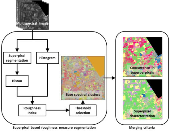
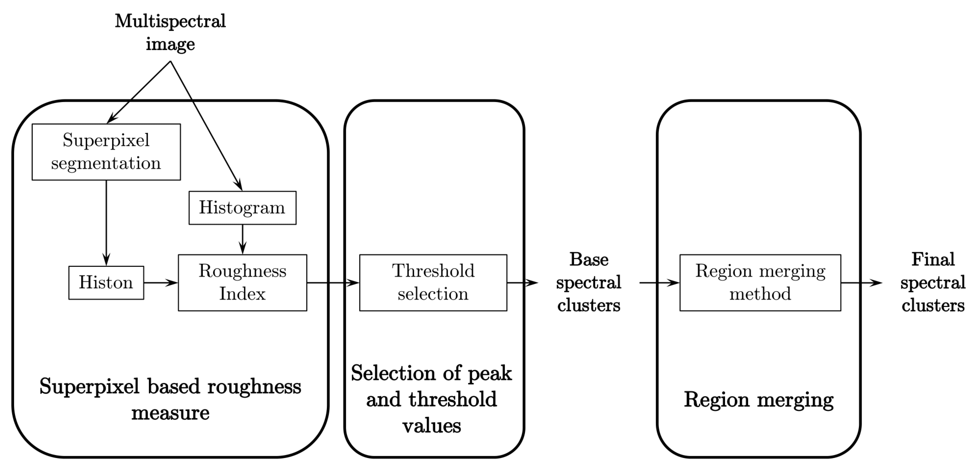
3.1. Superpixel-Based Roughness Measure in Multispectral Satellite Images

We propose the use of superpixels (in this case, using SLIC) to define the neighborhood for the histon creation and the superpixels’ local average standard deviation to provide the expanse for its color sphere. Although the original roughness index-based segmentation performs better than the methods based on traditional histograms and histons, as can be seen in [19], this method uses to calculate the histons a color sphere based on a fixed neighborhood (specifically, the 24 neighbors surrounding each pixel) and a fixed color distance. This small neighborhood, unrelated to the specific geometry of the image, tends to emphasize compact regions. As a result, color differences diffusely distributed or associated with narrow, elongated structures may appear under-represented in the histon and, therefore, in its derived roughness index.

In [30], scale-space representation of an RGB image is used as a means to adapt the pixels’ neighborhood to the local particularities of the image. In our case, we expect to exploit a prior superpixel segmentation of the multi-spectral image as a form to describe local similarities. Using this segmentation (specifically, an over-segmentation), we seek not only to create a natural set of neighborhoods for the histon generation, but also, as can be seen in the next section, to provide a tool to refine the results obtained by using the roughness index.

The use of superpixels as the neighborhood for the histon calculation guarantees a direct spatial relation between the pixel tested for its pertinence to the color sphere, respecting features and frontiers between areas present in the image. However, this is not the only advantage related to the use of superpixels. Regarding this aspect, superpixels allow one to define what we consider a homogeneous region, not based on a fixed value for any image, but adapted to their specific characteristics. Experimental results show that, since segmentation using superpixels already produces locally-homogeneous areas, the intensity average standard deviation of the superpixel-defined space can give us a threshold to globally quantify the local homogeneity. A pixel will be within the color sphere, if the distance between the average intensity of its belonging superpixel and the pixel intensity is below the average local standard deviation of the spectral plane in the superpixel-defined space, in each of its spectral components.

Let us denote the set of resulting superpixels in an image segmentation as $Cs=\{C{s}_1,C{s}_2,···,C{s}_{Ns}\}$, where $Ns$ is the total number of superpixels, $I(x_{C{s}_j},y_{C{s}_j},s_i)$ represents the centroid of the superpixel $C{s}_j$ in the spectral band $s_i\in S_p$ and $N{p}_j$ is the number of pixels in that superpixel; the similarity function $S_2\left(x,y\right)$ is defined as:

$$S_2\left(x,y\right)=\left\{\begin{array}{cc}1\hfill & \text{if}\forall s_i\in S_p{d}_{t{s}_i}\left(x,y\right)<E_{s_i}\hfill \\ 0\hfill & \text{otherwise}\hfill \end{array}\right.$$

(9)

$$d_{t{s}_i}\left(x,y\right)=\left|I(x,y,s_i)-I(x_{C{s}_j},y_{C{s}_j},s_i)\right|I(x,y,s_i)\in C{s}_j$$

(10)

$$E_{s_i}=\frac{1}{Ns}\sum _{j=1}^{Ns}\frac{1}{N{p}_j}\sum _{I\in C{s}_j}I(x,y,s_i)$$

(11)

Switching from a fixed radius to an area directly related to a pixel, the color distribution can be represented in a more accurate and natural way, as the neighborhood for each pixel, a superpixel, represents a real area within the image, related to its features. Furthermore, the superpixel segmentation enables the use of the local average standard deviation to adapt the metrics defining the color sphere to each image.

Each of the peaks of the roughness index represents a uniform region of the image in the same way as peaks in histograms do. The correct peak selection is the key to achieving good segmentation results. Small thresholds can cause many redundant segments on the spectral components, and an overly large threshold may miss important peaks for the segmentation.

In [19], a peak is defined as significant if its height is greater than 20% of the average value of the roughness index and the distance between peaks is greater than 10. However, multi-spectral satellite images present a specific challenge; it is usual that, for a spectral band, most of the intensity values appear concentrated in a narrow range, making this band under-represented in the final segmentation if a fixed distance value between peaks is used. This case can be detected by checking the distribution of values in the histogram using the corresponding quantiles. Thus, each histogram is checked and considered “cramped” if at least 90% of its intensity values are grouped in less than 50% of the total values’ range. In this case, the minimum possible distance between peaks is linearly lowered from the original value of $10*\left(max\right(I\left(s_i\right)-min\left(I\left(s_i\right)\right)$ to a minimum of $2*\left(max\right(I\left(s_i\right)-min\left(I\left(s_i\right)\right)$, when 90% of the values are grouped in less than 10% of the total span.

After selecting the significant peaks, the valleys are obtained by finding the minimum values between every two adjacent peaks. According to the location of peaks and valleys, the spectral clusters on each spectral component are formed and combined in a base segmentation.

3.2. Region Merging

Roughness index-based methods treat each spectral band individually and tend to highlight region homogeneity, generating more spectral clusters than histogram-based methods. The original method uses the algorithm proposed by Cheng et al. in [31] for region merging. This algorithm is essentially a color distance-based merging algorithm designed for color photography. Color distance, as can be seen in [32], is not a trivial concept, and its extension to a multispectral domain does not guarantee adequate results.

We propose two different merging methods, one pixel based, named co-occurrence in superperpixels, and one segment based (in this case superpixel), named superpixel characterization. Both share the same underlying structure; a similarity distance between the obtained spectral clusters is defined using its relation to the superpixel over-segmentation. This distance is used to construct a distance matrix between pairs of elements (the base spectral clusters or the superpixels). A hierarchical binary cluster tree showing the relations between elements can be created from this matrix using the UPGMA (unweighted pair group method with arithmetic mean) algorithm (see [33]). The resulting tree is a multilevel hierarchy, where clusters at one level are joined in one cluster at the next level. This structure allows one to decide the scale of clustering (in our case, the final number of clusters) that is most appropriate for an application.

3.2.1. Co-Occurrence in Superperpixels

As mentioned above, each superpixel represents a statistically-homogeneous area. This means that not only a limited number of the base spectral clusters are represented in any superpixel, but also that these clusters are going to be closely related in a perceptual sense. We can therefore address the region-merging problem as a problem of unsupervised clustering of spectral clusters, taking into account their co-occurrence inside each superpixel.

For a set of base spectral clusters $Sb=\{S{b}_1,S{b}_2,···,S{b}_{Nsb}\}$, where $Nsb$ represents the total number of base spectral clusters, we define the relation between the cluster $S{b}_m$ and the cluster $S{b}_n$ as the average percentage of area covered by $S{b}_n$ in each of the superpixels where the base spectral clusters $S{b}_m$ and $S{b}_n$ are both present, divided by the total percentage covered by $S{b}_n$ in the image. This relation is calculated for each pair of clusters to create a co-occurrence matrix $X(Nsb,Nsb)$ that can be directly fed to UPGMA, as can be seen in the following equation:

$$X\left(m,n\right)=\left\{\begin{array}{cc}0\hfill & \text{if}m=n\hfill \\ {\displaystyle \frac{1}{Ns{b}_n/(N*M)}\sum _{i=1}^{Ns}\frac{C{s}_i^{S{b}_n}}{N{p}_i}}\hfill & \text{otherwise}\hfill \end{array}\right.$$

(12)

where $Ns{b}_n$ is the number of pixels that belongs to the spectral cluster n and $C{s}_i^{S{b}_n}$ represents the pixels in the superpixel $C{s}_i$, which belongs to the spectral cluster $S{b}_n$.

3.2.2. Superpixel Characterization

The use of superpixels as a basis for OBIA (object-based image analysis) (see [34] or [35]) is a relatively recent development in satellite image analysis and appears as a useful way to improve classification performance without introducing too much additional computational costs. Since we already have started with superpixel segmentation, the idea of using those results as a starting point for analyzing the image seems an interesting opportunity, with the dual purpose of both region merging and to provide a low-level approximation for a possible OBIA analysis.

The original purpose of UPGMA was to construct taxonomic phenograms, trees that reflect the phenotypic similarities between species or groups of species. We can consider the superpixel set as a population composed of different subspecies, their phenotype characterized by the base spectral clusters present in each superpixel. Similar areas in the image will yield superpixels with a similar base spectral cluster distribution. Thus, we can consider the region-merging process an unsupervised clustering problem, using the distribution of the spectral clusters inside the superpixels as the base for a distance measure. Each superpixel in the set of resulting superpixels in segmentation, $Cs=\{C{s}_1,C{s}_2,···,C{s}_{Ns}\}$, can be described in relation to the set of base spectral clusters, $Sb=\{S{b}_1,S{b}_2,···,S{b}_{Nsb}\}$, as a sequence of values $Vs=\{V{s}_1,V{s}_2,···,V{s}_{Sbn}\}$ indicating the percentage of the area of each superpixel $C{s}_i$ covered by each of the base spectral clusters $S{b}_j$ (see Equation 13). To create the similarity matrix $X(Ns,Nsb)$ between superpixels to use with UPGMA, Spearman’s rank correlation is utilized as a measure of similarity between these sequences of values.

$$V{s}_i=\sum _{j=1}^{Ns}\frac{C{s}_i^{S{b}_j}}{N{p}_i}i\in 1,···,Ns$$

(13)

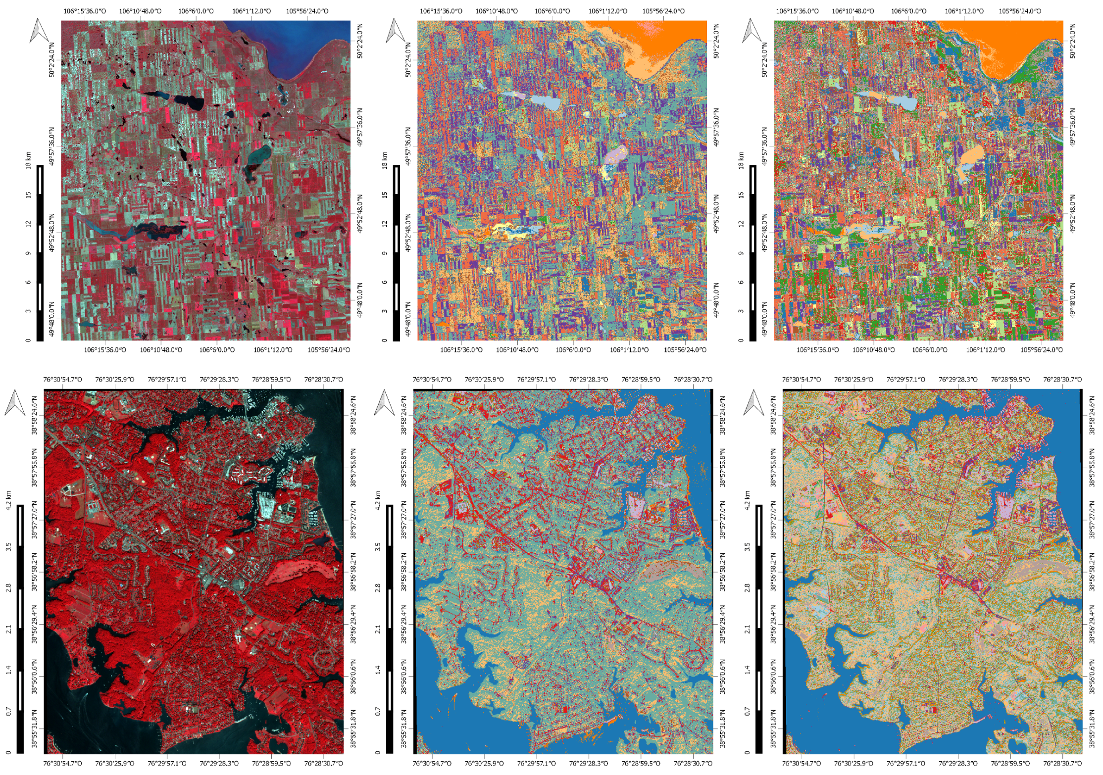
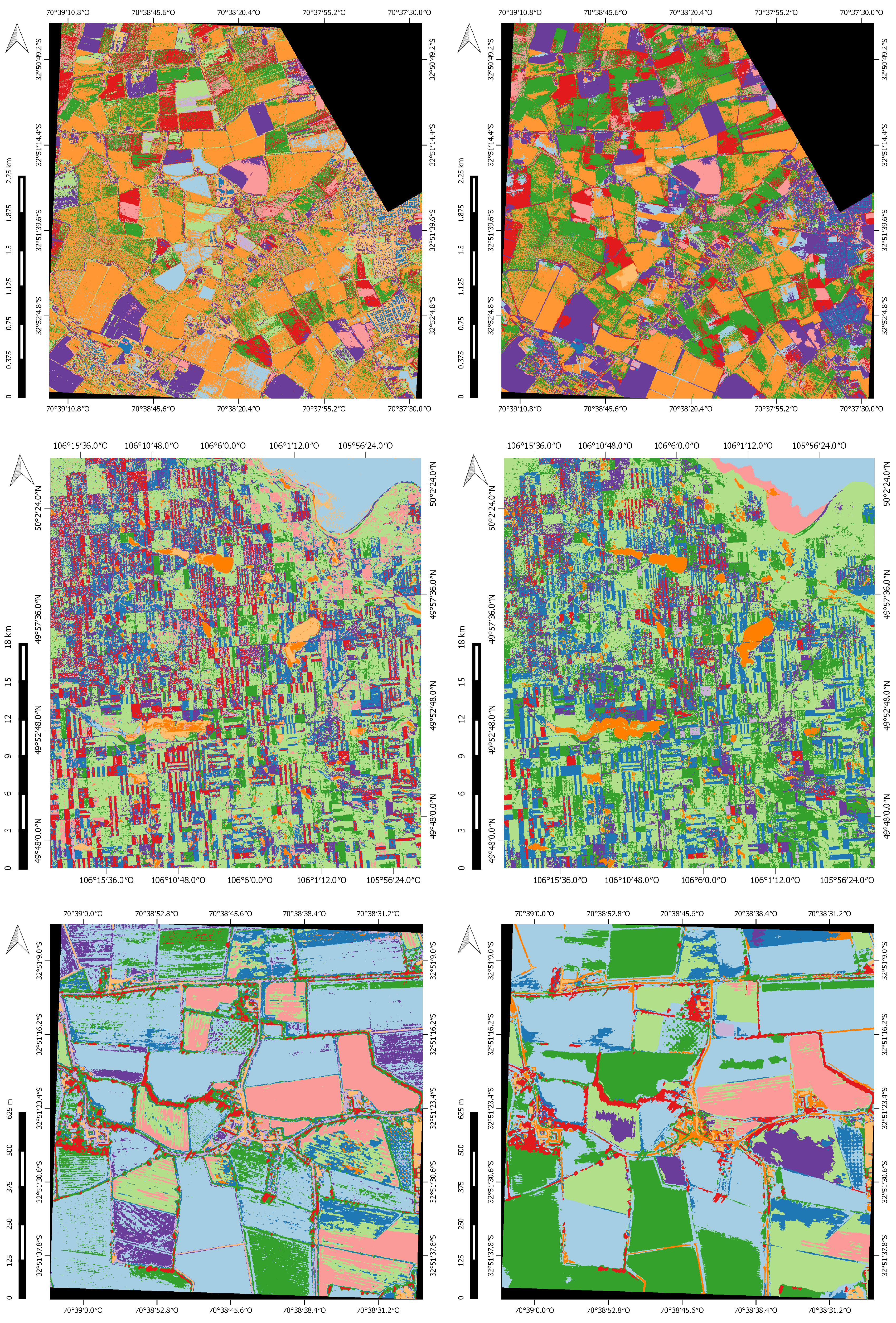
4. Study Area and Dataset

Six different satellite images have been selected as the test dataset for this method. Testing is performed using the blue, green, red and near-IR spectral bands.

The images CANADA1 and CANADA2 have been taken by the Landsat 7 satellite, with a spatial resolution of 30 meters. CANADA1 is an excerpt of 995 × 1100 pixels of an image taken on 23 August 1999 and shows the southwest area of Old Wives Lake, in Canada. CANADA2 forms part of an image acquired over Baffin Island on 11 July 2001, has a dimension of 1052 × 1224 pixels and shows the area surrounding Bowman Bay.

Images MARYLAND and ARGENTINA, with a spatial resolution of four meters, are from the OrbView-3 satellite. MARYLAND was taken on 12 August 2006 and represents a slice of 988 × 1218 pixels from the south area of Annapolis, in the state of Maryland, USA. ARGENTINA is part (1024 × 1148 pixels) of an image taken on 13 February 2006 and shows the southwest region of the village of Gobernador Costa.

Image CHILE1 is an image registered by the satellite Worldview-2, its multispectral sensor providing a 1.8-meter resolution. CHILE1 is a 2048 × 2048 pixels image taken on 11 September 2011. The area corresponds to a rural zone located in the Valparaiso region in Comuna de Los Andes, Chile.

Image CHILE2 is an excerpt of 1388 × 1350 pixels of an image taken by the QuickBird-2 satellite, with a resolution of 2.4 meters per pixel, acquired on 3 December 2011, corresponding to an area in Comuna de Calle Larga, in the Valparaiso region, Chile.

5. Results and Discussion

Quality evaluation for image segmentation is a known hard problem, especially when there is not a ground truth to compare. We can propose a set of desirable and measurable characteristics in a segmentation (as can be seen in the seminal work of Haralick et al. in [36]) that can be calculated and used as a criteria for an unsupervised quantitative evaluation. Unsupervised quantitative evaluation has distinctive advantages, is completely objective and, perhaps the most critical, requires no reference image. However, unsupervised quantitative criteria are not intended to provide the absolute quality of a segmentation, as only a specific set of features in an image are really measurable. On the other hand, although each problem has its distinct standard for a good segmentation, a qualitative evaluation is also possible, and despite its evident human-bias, differences between adequate segmentation and an inferior one are usually noticeable and describable. Therefore, we will perform an unsupervised evaluation and a qualitative assessment. We will compare the complete superpixel-based roughness segmentation method to the original segmentation method [19] and the two proposed merging algorithms with the original color distance-merging algorithm in [31]. Results presented in this paper have been obtained using experimental, in-house-developed software running on the MATLAB platform.

As the proposed method is based on the detection of perceptually-uniform spectral regions in the image, the unsupervised quantitative evaluation will be performed on the inter-region variability and intra-region uniformity. As evaluation criterion, the well-known aggregate Levine and Nazif [37] criterion has been chosen, which takes into account both the intra-region uniformity (as one minus the normalized variance of colors inside each region) and inter-region disparity (as the weighted sum of the contrasts of the regions, normalized using the percentage of shared edges between classes). Intra-region uniformity and inter-region disparity are complementary measures that evaluate the uniformity and distinctiveness of the regions resulting from a segmentation. This criterion increases its value as the segmentation quality increases.

5.1. Superpixel-Based Roughness Segmentation Evaluation

Table 1 shows the numbers of spectral clusters obtained by the superpixel-based roughness method and the results of the original roughness index-based method, compared to the results of a histogram-based threshold method before the region-merging phase, both per spectral band and for the final, combined result. We can observe how, as they take into account the spatial distribution of the image, both the original roughness index method of Mushrif and Ray and the proposed superpixel-based roughness index method usually provide a considerably larger number of spectral clusters for each spectral component and for the final segmentation than the histogram multi-band segmentation and how the presented method usually outperforms the original one. Although this is not a guarantee of a better segmentation, especially when there is going to be a merging phase to reduce the final number of base spectral clusters, it opens the possibility of a more accurate representation of the nuances and details in the image.

Table 1. Comparison of the numbers of spectral clusters yielded by the proposed method with the results of a histogram-based thresholding method and the results of the roughness index-based method, both per spectral band and the final, combined result.

Image	Method	Number of Clusters					Image	Method	Number of Clusters
		Blue	Green	Red	Infra	Final			Blue	Green	Red	Infra	Final
CHILE2	Histogram	3	4	5	9	63	CHILE1	Histogram	4	6	7	6	80
	Roughness index	25	20	26	16	141		Roughness index	10	9	11	13	121
	Superpixel roughness index	17	21	22	16	171		Superpixel roughness index	10	11	12	13	125
MARYLAND	Histogram	8	10	11	11	178	ARGENTINA	Histogram	1	5	5	9	76
	Roughness index	13	13	14	9	88		Roughness index	10	12	13	16	174
	Superpixel roughness index	18	19	23	14	177		Superpixel roughness index	11	12	16	11	176
CANADA2	Histogram	2	1	2	2	9	CANADA1	Histogram	2	1	2	2	7
	Roughness index	4	5	4	4	38		Roughness index	11	11	9	6	121
	Superpixel roughness index	12	13	14	18	188		Superpixel roughness index	10	12	9	8	110

Table 1. Comparison of the numbers of spectral clusters yielded by the proposed method with the results of a histogram-based thresholding method and the results of the roughness index-based method, both per spectral band and the final, combined result.

Image	Method	Number of Clusters					Image	Method	Number of Clusters
		Blue	Green	Red	Infra	Final			Blue	Green	Red	Infra	Final
CHILE2	Histogram	3	4	5	9	63	CHILE1	Histogram	4	6	7	6	80
	Roughness index	25	20	26	16	141		Roughness index	10	9	11	13	121
	Superpixel roughness index	17	21	22	16	171		Superpixel roughness index	10	11	12	13	125
MARYLAND	Histogram	8	10	11	11	178	ARGENTINA	Histogram	1	5	5	9	76
	Roughness index	13	13	14	9	88		Roughness index	10	12	13	16	174
	Superpixel roughness index	18	19	23	14	177		Superpixel roughness index	11	12	16	11	176
CANADA2	Histogram	2	1	2	2	9	CANADA1	Histogram	2	1	2	2	7
	Roughness index	4	5	4	4	38		Roughness index	11	11	9	6	121
	Superpixel roughness index	12	13	14	18	188		Superpixel roughness index	10	12	9	8	110

Table 2 presents the results of the unsupervised quantitative evaluation from the aggregate Levine and Nazif criterion, showing results for intra-region uniformity, inter-region disparity and the total aggregate. Intra-region uniformity and the aggregate criterion are clearly favorable for the superpixel-based roughness method, although the use of this method shows no advantage from the point of view of inter-region disparity. Therefore, we can affirm that the use of superpixel-based roughness produces significantly more homogeneous segments than the original method, but no more distinctly. Taking into account both intra-regional uniformity and inter-regional disparity, the proposed method shows a clear advantage. In any case, it should be noted that generally, the numerical differences in this quantitative evaluation between the two methods are not very pronounced.

Experimental results show a relation between the image homogeneity and the quantitative results (homogeneity defined as a measure of the closeness of the distribution of elements in a gray-level co-occurrence matrix to its diagonal, in each spectral plane of the image). The original method tends to perform better for images with a bigger homogeneity value. This relationship would be consistent with expectations, as the problems with the original method are associated with small structures or complex areas of terrain present in the image.

Table 2. Levine and Nazif evaluation criterion results for the original algorithm and the proposed method, ordered by segmentation and merging region methods for 5, 10 and 15 final spectral clusters (where N. Clusters is the number of final spectral clusters, C. Dist is the color distance, Coo. Sup. represents the co-occurrence in the superpixel method and Sup. Ch. is the superpixel characterization method). The best results for each criteria (intra-region uniformity, inter-region variability and the aggregate values) for each segmentation appear highlighted in dark grey. The best results taking into account only the segmentation method are also shown in light grey.

		Intra-Region Uniformity						Inter-Region Variability						Aggregate Value
		Roughness Index			Superpixel-Based Roughness			Roughness Index			Superpixel-Based Roughness			Roughness Index			Superpixel-Based Roughness
Image	N.Clusters	C. Dist	Coo. Sup.	Sup. Ch.	C. Dist	Coo. Sup.	Sup. Ch.	C. Dist	Coo. Sup.	Sup. Ch.	C. Dist	Coo. Sup.	Sup. Ch.	C. Dist	Coo. Sup.	Sup. Ch.	C. Dist	Coo. Sup.	Sup. Ch.
CANADA1	5	0.7343	0.6650	0.7011	0.7809	0.7332	0.7300	0.2137	0.1307	0.2020	0.2490	0.2080	0.2151	0.4740	0.3978	0.4515	0.5150	0.4706	0.4725
	10	0.6025	0.6648	0.6144	0.6852	0.7013	0.6484	0.1787	0.1715	0.1752	0.1726	0.1755	0.1785	0.3906	0.4182	0.3948	0.4289	0.4384	0.4134
	15	0.6274	0.6432	0.5228	0.6495	0.6357	0.5457	0.1712	0.1624	0.1753	0.1716	0.1654	0.1779	0.3993	0.4028	0.3491	0.4105	0.4005	0.3618
CANADA2	5	0.8764	0.7670	0.8594	0.8306	0.8564	0.8310	0.1640	0.1711	0.2844	0.1761	0.1636	0.1897	0.5202	0.4690	0.5719	0.5034	0.5100	0.5103
	10	0.7678	0.6676	0.7081	0.8307	0.8158	0.7611	0.1877	0.1780	0.1745	0.1753	0.1703	0.1739	0.4777	0.4228	0.4413	0.5030	0.4931	0.4675
	15	0.6960	0.6725	0.6562	0.8132	0.8001	0.7003	0.1741	0.1739	0.1749	0.1749	0.1765	0.1764	0.4350	0.4232	0.4156	0.4940	0.4882	0.4383
ARGENTINA	5	0.7871	0.7939	0.7045	0.7795	0.7291	0.6945	0.1770	0.1791	0.1819	0.2142	0.1685	0.1668	0.4821	0.4865	0.4432	0.4969	0.4488	0.4306
	10	0.7288	0.6973	0.6152	0.6975	0.6278	0.5389	0.1656	0.1770	0.1722	0.1742	0.1724	0.1633	0.4472	0.4372	0.3937	0.4359	0.4001	0.3511
	15	0.6563	0.6649	0.4498	0.6423	0.6105	0.4154	0.1698	0.1687	0.1705	0.1696	0.1693	0.1618	0.4130	0.4168	0.3102	0.4060	0.3899	0.2886
MARYLAND	5	0.8541	0.8943	0.8567	0.8632	0.9003	0.8495	0.4556	0.4391	0.4158	0.3856	0.4739	0.4801	0.6548	0.6667	0.6362	0.6244	0.6871	0.6648
	10	0.8015	0.8094	0.6350	0.8323	0.8881	0.7592	0.4428	0.4377	0.4123	0.4193	0.4632	0.4688	0.6221	0.6235	0.5237	0.6258	0.6757	0.6140
	15	0.7504	0.7314	0.5337	0.8213	0.8896	0.7189	0.4337	0.4388	0.4120	0.4171	0.4571	0.4582	0.5921	0.5851	0.4729	0.6192	0.6734	0.5886
CHILE1	5	0.8233	0.8817	0.8471	0.8187	0.8851	0.8312	0.3124	0.2959	0.2943	0.2986	0.2825	0.2973	0.5679	0.5888	0.5707	0.5586	0.5838	0.5642
	10	0.8088	0.8408	0.8328	0.8013	0.8744	0.8074	0.2897	0.2895	0.2909	0.3031	0.2894	0.2923	0.5492	0.5651	0.5618	0.5522	0.5819	0.5498
	15	0.7984	0.8276	0.7331	0.8020	0.8378	0.7808	0.2869	0.2856	0.2895	0.2886	0.2851	0.2885	0.5427	0.5566	0.5113	0.5453	0.5614	0.5347
CHILE2	5	0.7568	0.8594	0.8967	0.7515	0.8239	0.9053	0.2310	0.2002	0.2302	0.2363	0.2048	0.1969	0.4939	0.5298	0.5635	0.4939	0.5143	0.5511
	10	0.7463	0.8547	0.8009	0.7439	0.8125	0.8989	0.2044	0.1931	0.2031	0.1977	0.1972	0.2004	0.4753	0.5239	0.5020	0.4708	0.5048	0.5496
	15	0.7449	0.7664	0.7859	0.7310	0.8041	0.8068	0.2017	0.1897	0.2033	0.1972	0.1929	0.1958	0.4733	0.4781	0.4946	0.4641	0.4985	0.5013

Table 2. Levine and Nazif evaluation criterion results for the original algorithm and the proposed method, ordered by segmentation and merging region methods for 5, 10 and 15 final spectral clusters (where N. Clusters is the number of final spectral clusters, C. Dist is the color distance, Coo. Sup. represents the co-occurrence in the superpixel method and Sup. Ch. is the superpixel characterization method). The best results for each criteria (intra-region uniformity, inter-region variability and the aggregate values) for each segmentation appear highlighted in dark grey. The best results taking into account only the segmentation method are also shown in light grey.

		Intra-Region Uniformity						Inter-Region Variability						Aggregate Value
		Roughness Index			Superpixel-Based Roughness			Roughness Index			Superpixel-Based Roughness			Roughness Index			Superpixel-Based Roughness
Image	N.Clusters	C. Dist	Coo. Sup.	Sup. Ch.	C. Dist	Coo. Sup.	Sup. Ch.	C. Dist	Coo. Sup.	Sup. Ch.	C. Dist	Coo. Sup.	Sup. Ch.	C. Dist	Coo. Sup.	Sup. Ch.	C. Dist	Coo. Sup.	Sup. Ch.
CANADA1	5	0.7343	0.6650	0.7011	0.7809	0.7332	0.7300	0.2137	0.1307	0.2020	0.2490	0.2080	0.2151	0.4740	0.3978	0.4515	0.5150	0.4706	0.4725
	10	0.6025	0.6648	0.6144	0.6852	0.7013	0.6484	0.1787	0.1715	0.1752	0.1726	0.1755	0.1785	0.3906	0.4182	0.3948	0.4289	0.4384	0.4134
	15	0.6274	0.6432	0.5228	0.6495	0.6357	0.5457	0.1712	0.1624	0.1753	0.1716	0.1654	0.1779	0.3993	0.4028	0.3491	0.4105	0.4005	0.3618
CANADA2	5	0.8764	0.7670	0.8594	0.8306	0.8564	0.8310	0.1640	0.1711	0.2844	0.1761	0.1636	0.1897	0.5202	0.4690	0.5719	0.5034	0.5100	0.5103
	10	0.7678	0.6676	0.7081	0.8307	0.8158	0.7611	0.1877	0.1780	0.1745	0.1753	0.1703	0.1739	0.4777	0.4228	0.4413	0.5030	0.4931	0.4675
	15	0.6960	0.6725	0.6562	0.8132	0.8001	0.7003	0.1741	0.1739	0.1749	0.1749	0.1765	0.1764	0.4350	0.4232	0.4156	0.4940	0.4882	0.4383
ARGENTINA	5	0.7871	0.7939	0.7045	0.7795	0.7291	0.6945	0.1770	0.1791	0.1819	0.2142	0.1685	0.1668	0.4821	0.4865	0.4432	0.4969	0.4488	0.4306
	10	0.7288	0.6973	0.6152	0.6975	0.6278	0.5389	0.1656	0.1770	0.1722	0.1742	0.1724	0.1633	0.4472	0.4372	0.3937	0.4359	0.4001	0.3511
	15	0.6563	0.6649	0.4498	0.6423	0.6105	0.4154	0.1698	0.1687	0.1705	0.1696	0.1693	0.1618	0.4130	0.4168	0.3102	0.4060	0.3899	0.2886
MARYLAND	5	0.8541	0.8943	0.8567	0.8632	0.9003	0.8495	0.4556	0.4391	0.4158	0.3856	0.4739	0.4801	0.6548	0.6667	0.6362	0.6244	0.6871	0.6648
	10	0.8015	0.8094	0.6350	0.8323	0.8881	0.7592	0.4428	0.4377	0.4123	0.4193	0.4632	0.4688	0.6221	0.6235	0.5237	0.6258	0.6757	0.6140
	15	0.7504	0.7314	0.5337	0.8213	0.8896	0.7189	0.4337	0.4388	0.4120	0.4171	0.4571	0.4582	0.5921	0.5851	0.4729	0.6192	0.6734	0.5886
CHILE1	5	0.8233	0.8817	0.8471	0.8187	0.8851	0.8312	0.3124	0.2959	0.2943	0.2986	0.2825	0.2973	0.5679	0.5888	0.5707	0.5586	0.5838	0.5642
	10	0.8088	0.8408	0.8328	0.8013	0.8744	0.8074	0.2897	0.2895	0.2909	0.3031	0.2894	0.2923	0.5492	0.5651	0.5618	0.5522	0.5819	0.5498
	15	0.7984	0.8276	0.7331	0.8020	0.8378	0.7808	0.2869	0.2856	0.2895	0.2886	0.2851	0.2885	0.5427	0.5566	0.5113	0.5453	0.5614	0.5347
CHILE2	5	0.7568	0.8594	0.8967	0.7515	0.8239	0.9053	0.2310	0.2002	0.2302	0.2363	0.2048	0.1969	0.4939	0.5298	0.5635	0.4939	0.5143	0.5511
	10	0.7463	0.8547	0.8009	0.7439	0.8125	0.8989	0.2044	0.1931	0.2031	0.1977	0.1972	0.2004	0.4753	0.5239	0.5020	0.4708	0.5048	0.5496
	15	0.7449	0.7664	0.7859	0.7310	0.8041	0.8068	0.2017	0.1897	0.2033	0.1972	0.1929	0.1958	0.4733	0.4781	0.4946	0.4641	0.4985	0.5013

From a qualitative point of view, we are going to compare the results of the original method adapted to multi-spectral images (including adaptive selection of peaks and a lightly-modified merging algorithm proposed in [31] to control the final number of regions) and our superpixel-based roughness index using the proposed per pixel co-occurrence in the superpixel region-merging method (as both segmentation methods are pixel-based methods). Since the general conclusions of these tests do not change significantly regardless of the combinations between segmentation methods and region-merging methods, the region-merging methods results, behaviors and performance will be discussed independently in the next subsection. The color for the provided results has been chosen to maximize the images’ legibility, using [38], and has no further meaning.

The main difference between the two segmentation methods, before the area-merging phase, is what is understood as the neighborhood of a pixel and, therefore, how and where the similarity function defining the color sphere for the histon calculation is applied. As we have mentioned previously, the original roughness-based segmentation defines the neighborhood of a pixel as a small, fixed area around it. Although it is able to detect the homogeneity associated with small variations in well-defined areas, heterogeneous regions or small, but significant differences between areas tend to appear under-represented. On the other hand, the use of superpixels effectively isolates the regions present in the image in their own neighborhoods.

Figure 2 presents the results for CHILE1 (upper row) and CANADA1 (lower row) for 15 final spectral classes. As can be seen, in the image CHILE1, the use of superpixels as the neighborhood (right image) allows one to better discern differences inside and between crop areas. Results for the image CANADA1 show that, despite the original method presented in [19] showing more variety in compact areas, such as the small lakes, the subtle differences associated with the central terrain and the long, narrow features related to water streams are properly represented. As a consequence, for both CANADA1 and CHILE1, the proposed method better reflects the distribution of regions in the images.

Figure 3 shows the results from the images CANADA2 and MARYLAND (middle column with the original method, right column with the superpixel-based method). CANADA2 (upper row) is a low spatial resolution image of an agricultural area, showing a notable variety in terrain types and crops; MARYLAND (lower row) is a high spatial resolution urban image presenting a heterogeneous set of built-up structures, vegetation, bare soil and water areas. Relevant regions in both images appear divided and spread; as a set of small crop fields in CANADA2 and as a network of buildings and roads in MARYLAND. Treating this kind of image as a set of isolated, feature-based neighborhoods, we can get a better representation of the features presented in the terrain, and we are able, for the same number of final spectral clusters, to better capture the differences between regions, regardless of their distribution in the image. Again, the original method tends to over-represent compact areas in the results, as the lake in the upper right of CANADA2 or the golf course in the middle right part of the MARYLAND image. On the other hand, the use of superpixels as the neighborhood keeps the general structure of the image, represented in CANADA2 by the differences between fields and in MARYLAND by the differences in the forest areas and urban zones. In these images, this is also reflected in the amount of base spectral clusters that are obtained before the merging step, significantly bigger for the proposed method, as is presented in Table 1.

Figure 2. Results for image CHILE1 are displayed in the upper row and for CANADA1 in the lower row. First column: false color composite NIR-G-R. Results for the original method and proposed method for 15 final clusters are displayed in the second and third columns, respectively. Colors have no special meaning.

Figure 2. Results for image CHILE1 are displayed in the upper row and for CANADA1 in the lower row. First column: false color composite NIR-G-R. Results for the original method and proposed method for 15 final clusters are displayed in the second and third columns, respectively. Colors have no special meaning.

Figure 3. Results for image CANADA2 are displayed in the upper row and for MARYLAND in the lower row. First column: false color composite NIR-G-R. Results for the original method and proposed method for 15 final clusters are displayed in the second and third columns, respectively. Colors have no special meaning.

Figure 3. Results for image CANADA2 are displayed in the upper row and for MARYLAND in the lower row. First column: false color composite NIR-G-R. Results for the original method and proposed method for 15 final clusters are displayed in the second and third columns, respectively. Colors have no special meaning.

In Figure 4, we also observe another problem derived from the limited definition of the neighborhood in the original method. Details in the image spectrally close to homogeneous areas, but otherwise unrelated can be segmented as part of these areas, as can be seen in MARYLAND, with sea areas and the shadows present in the image, and in CANADA2, with the shallow waters of the lake and parts of the nearby forest. These artifacts are not present in the results of our proposed method. As we will see in the next subsection, this problem can be also produced, or be exacerbated, by using the color distance as the region-merging method.

Figure 4. Upper row: Details of the upper right corner of the image CANADA2. Excerpt position (left image), results for the original method (middle image) and for the proposed method (right image). Lower row: details of the golf course area of the image MARYLAND. Excerpt position (left image), results for the original method (middle image) and for the proposed method (right image). Colors have no special meaning.

Figure 4. Upper row: Details of the upper right corner of the image CANADA2. Excerpt position (left image), results for the original method (middle image) and for the proposed method (right image). Lower row: details of the golf course area of the image MARYLAND. Excerpt position (left image), results for the original method (middle image) and for the proposed method (right image). Colors have no special meaning.

5.2. Merging Strategies’ Evaluation

From the results of the quantitative assessment in Table 2, we can not really say that a region-merging method is better or worse than the others. Both the aggregate Levine and Nazif criterion and the intra-region uniformity alone show better results when they are applied to the results of co-occurrence in the superpixel method, although differences are not enough to make it the obvious choice. From the standpoint of inter-regional disparities, none of the methods stand. Taking into account only the qualitative assessment, we can conclude that neither the color distance methods nor the proposed ones especially stand out, with the results depending more on the specific image than the area-merging method. Finally, again, numerical differences between methods are not very significant.

The use of co-occurrence in superpixels replaces a spectral proximity-based method with one based on spatial proximity, with the idea that the spectral proximity has already been taken into account both by the superpixel over-segmentation and the roughness index segmentation. Whereas this may lead to the merging of base spectral clusters associated with features in the image with a strong co-occurrence relationship, the underlying structure of the image is better maintained. In Figure 5, in the image CHILE2 (upper row), although both methods maintain the overall structure of the image, co-occurrence in superpixels (right column) better represents relevant differences between and inside the different crop fields. In the image ARGENTINA (lower row), the spectral differences within the remaining ponds of water associated with the presence of vegetation are greater than those between the different types of terrain, and there is an obvious spatial relationship between different zones present in the ponds. As a result, the original color distance method (middle column) preserves the subtle differences in the ponds at the expense of the areas presented in the rest of the terrain, while the use of co-occurrence in superpixels (right column), although merging ponds into a single area, maintains the general differences in the terrain.

Differences between region-merging methods are especially significant when we are looking for a segmentation composed of a small number of areas. In Figure 6, we can observe the results of a segmentation with five final spectral clusters for the images CHILE2 (upper row) and ARGENTINA (lower row), both for the color distance (left column) and co-occurrence in the superpixel (right column) region-merging method. In the image ARGENTINA, color distance as a region-merging method focuses on the image details, essentially leaving only the prominent parts of the water ponds and the rocky hills. On the other hand, using co-occurrence in superpixels, the main areas in the image remain perfectly identifiable. In the image CHILE2, we see, for example, that despite losing details, like individual structures in urban areas (in this case formed by the spectral clusters associated mainly with roofing asphalt and dry land), the urban areas remain as a distinct area.

Another consequence of using a spatial proximity-based region-merging method is that not spatially-related, but otherwise similar base spectral clusters will be kept separate. We can see in Figure 7 how the use of color distance merges water and shaded patches in the image MARYLAND, as they have a similar spectral distribution. However, by using co-occurrence in superpixels, these two distinct features remain separate, as there is not a clear co-occurrence relation between water and shadows in the image.

Figure 5. Region-merging methods’ comparison; results for image CHILE2 (15 final spectral clusters) are displayed in the upper row and for ARGENTINA (10 final spectral clusters) in the lower row. First column: false color composite NIR-G-R. Results for the color distance region-merging method and co-occurrence in superpixels region-merging method are displayed in the second and third column, respectively. Colors have no special meaning.

Figure 5. Region-merging methods’ comparison; results for image CHILE2 (15 final spectral clusters) are displayed in the upper row and for ARGENTINA (10 final spectral clusters) in the lower row. First column: false color composite NIR-G-R. Results for the color distance region-merging method and co-occurrence in superpixels region-merging method are displayed in the second and third column, respectively. Colors have no special meaning.

Figure 6. Region-merging methods’ comparison; five final spectral clusters. Upper row: image CHILE2. Color distance (left image) and co-occurrence in superpixels (right image). Lower row: image ARGENTINA. Color distance (left image) and co-occurrence in superpixels (right image). Colors have no special meaning.

Figure 6. Region-merging methods’ comparison; five final spectral clusters. Upper row: image CHILE2. Color distance (left image) and co-occurrence in superpixels (right image). Lower row: image ARGENTINA. Color distance (left image) and co-occurrence in superpixels (right image). Colors have no special meaning.

The second region-merging method, superpixel characterization, is a segment-based method that takes advantage of the distribution of the base spectral clusters to describe each superpixel as a sequence of values. Some examples of the results of merging regions using superpixel characterization compared to area merging using co-occurrence in superpixels can be observed in Figure 8 and Figure 9 (the left column shows co-occurrence in superpixel results; the right column shows superpixel characterization results). As a segment-based method, superpixel characterization avoids the “salt and pepper” effect associated with pixel-based methods that can occur in complex or high resolution images with a high local variance, as can be seen in the image CHILE2 and CANADA2 (Figure 8) or ARGENTINA and MARYLAND (Figure 9). Crop fields in the images CHILE1 and CHILE2 (Figure 8) show how the use of superpixel characterization also prioritizes the general differences between well-defined areas over the segmentation of small details.

On the other hand, even with a strong spatial component related to the superpixel segmentation, the superpixel characterization method is based on spectral proximity, so there is a tendency to emphasize the homogeneity in large or poorly-defined areas, as can be seen in images ARGENTINA or CANADA1 (Figure 9). Furthermore, in image CANADA1, water streams appear fragmented or completely ignored, as features represented by small or irregular areas can be lost using superpixel characterization, especially if these have not been reflected in the superpixel segmentation. Anyway, compared to the color distance area-merging method, the structure of the image appears better defined and spectrally closed, but unrelated regions remain differentiated.

Figure 7. Region-merging methods’ comparison. Results for the image MARYLAND using the color distance region-merging method (left image) and the co-occurrence in the superpixel method (right image) for five final spectral clusters. Colors have no special meaning.

Figure 7. Region-merging methods’ comparison. Results for the image MARYLAND using the color distance region-merging method (left image) and the co-occurrence in the superpixel method (right image) for five final spectral clusters. Colors have no special meaning.

Figure 8. Region-merging methods’ comparison. Co-occurrence in superpixels results in the left column and superpixel characterization in the right column. Upper row: image CHILE2 (10 final spectral clusters). Middle row: image CANADA2 (10 final spectral clusters). Lower row: image CHILE1 (10 final spectral clusters). Colors have no special meaning.

Figure 8. Region-merging methods’ comparison. Co-occurrence in superpixels results in the left column and superpixel characterization in the right column. Upper row: image CHILE2 (10 final spectral clusters). Middle row: image CANADA2 (10 final spectral clusters). Lower row: image CHILE1 (10 final spectral clusters). Colors have no special meaning.

Figure 9. Region-merging methods’ comparison. Co-occurrence in superpixels results in the left column and superpixel characterization in the right column. Upper row: image ARGENTINA (15 final spectral clusters). Middle row: image CANADA1 (10 final spectral clusters). Lower row: image MARYLAND (10 final spectral clusters). Colors have no special meaning.

Figure 9. Region-merging methods’ comparison. Co-occurrence in superpixels results in the left column and superpixel characterization in the right column. Upper row: image ARGENTINA (15 final spectral clusters). Middle row: image CANADA1 (10 final spectral clusters). Lower row: image MARYLAND (10 final spectral clusters). Colors have no special meaning.

6. Conclusions

A method for the segmentation of multi-spectral images, a heavy modified evolution of the method proposed in [19], has been presented. This method explores the idea of evaluating the local spectral homogeneity of an image using a superpixel segmentation as a way to create a natural neighborhood for each pixel. The algorithm is divided into three stages. In the first stage, the superpixel-based roughness index of each of the spectral components of the image is computed. In the second stage, an initial image segmentation is created using the significant peaks and valleys of the roughness index. The third stage involves region merging, as the initial result represents a spectral over-segmentation of the image. For this second step, different methods (one pixel related, one segment related) are presented in order to maintain control of the total number of segments produced by the method, both taking advantage of the previous superpixel segmentation.

From a quantitative point of view, the developed method shows an evident advantage when intra-regional homogeneity is measured, and although this advantage does not extend to inter-regional disparity, when both measures are used as an aggregate quality measure, the results are clearly favorable for the use of superpixels. Therefore, we can affirm that the use of superpixel-based roughness produces significantly more homogeneous segments than the original method, but no more distinctly. The same quality measure applied to the region-merging methods’ results does not show a clear “winner”. Taking into account the disparity between multispectral sensors, pixel scale and the differences in the types of terrain presented in the test set, these results are in line with expectations.

Comparing the results between the original method and ours, we can conclude that the superpixel-based roughness index allows one to better capture differences associated with fragmented and complex areas or subtle spectral differences associate with bigger, but spatially-unrelated areas. Both proposed merging area methods better maintain the general structure of the image regardless of the number of final spectral clusters and keep separated spectrally-close, but in other ways unrelated, regions in the image.

The use of the presented segmentation algorithm is not tied to any kind of multi-spectral sensor, but it is rather a general approach for the combination of spatial and spectral information in image segmentation. Therefore, the algorithm may be easily adapted to different types of multi-spectral or multi-band images. The problem of optimal parameter selection for satellite image segmentation using SLIC is kept out of the scope of this paper (some ideas about the optimal scale selection for superpixels can be seen in [39]). Results so far show that the influence of the superpixel segmentation should be further explored. This is applicable not only in relation to the SLIC parameters, but also if the segmentation is performed individually for each spectral plane of the image or if a specific spectral plane is given priority. Future lines of research include the extension of the proposed method to a generalization of rough-set theory, as is proposed in [40]. We also plan to extend the proposed method to the hyperspectral domain.

References

1. Friedman, N.; Russell, S. Image segmentation in video sequences: A probabilistic approach. In Proceedings of the Thirteenth Conference on Uncertainty in Artificial Intelligence, Providence, RI, USA, 1–3 August 1997.
2. Fröhlich, B.; Bach, E.; Walde, I.; Hese, S.; Schmullius, C.; Denzler, J. Land cover classification of satellite images using contextual information. ISPRS Ann. Photogramm., Remote Sens. Spat. Inf. Sci. 2013, II-3/W1, 1–6. [Google Scholar] [CrossRef]
3. Pal, N.R.; Pal, S.K. A review on image segmentation techniques. Pattern Recognit. 1993, 26, 1277–1294. [Google Scholar] [CrossRef]
4. Lambert, P.; Macaire, L. Filtering and segmentation: The specificity of color images. In Proceedings of the First International Conference on Color in Graphics and Image Processing (CGIP), Saint-Etienne, France, 1–4 October 2000.
5. Banerjee, B.; Surender, V.; Buddhiraju, K. Satellite image segmentation: A novel adaptive mean-shift clustering based approach. In Proceedings of 2012 IEEE International Conference on Geoscience and Remote Sensing Symposium (IGARSS), Munich, German, 22–27 July 2012.
6. Zhang, H.; Fritts, J.E.; Goldman, S.A. Image segmentation evaluation: A survey of unsupervised methods. Comput. Vis. Image Underst. 2008, 110, 260–280. [Google Scholar] [CrossRef]
7. Al-amri, S.S.; Kalyankar, N.V.; D., K.S. Image Segmentation by Using Threshold Techniques. Available online: http://arxiv.org/abs/1005.4020 (accessed on 16 April 2015).
8. He, S.; Ni, J.; Wu, L.; Wei, H.; Zhao, S. Image threshold segmentation method with 2-D histogram based on multi-resolution analysis. In Proceedings of 4th International Conference on Computer Science & Education, Nanning, China, 25–28 July 2009.
9. Koonsanit, K.; Jaruskulchai, C.; Eiumnoh, A. Parameter-free K-means clustering algorithm for satellite imagery application. In Proceedings of 2012 International Conference on Information Science and Applications, Suwon, South Korea, 23–25 May 2012.
10. Yugander, P.; Sheshagiri, B.; Sunanda, K.; Susmitha, E. Multiple kernel fuzzy C-means algorithm with ALS method for satellite and medical image segmentation. In Proceedings of 2012 International Conference on Devices, Circuits and Systems, Coimbatore, India, 15–16 March 2012.
11. Tran, T.; Wehrens, R.; Buydens, L. Knn density-based clustering for high dimensional multispectral images. In Proceedings of 2nd GRSS/ISPRS Joint Workshop on Remote Sensing and Data Fusion over Urban Areas, Berlin, Germany, 22–23 May 2003.
12. Paclìk, P.; Duin, R.; van Kempen, G.; Kohlus, R. Segmentation of multi-spectral images using the combined classifier approach. Image Vis. Comput. 2003, 21, 473–482. [Google Scholar] [CrossRef]
13. Haralick, R.; Dinstein, I. A spatial clustering procedure for multi-image data. IEEE Trans. Circ. Syst. 1975, 22, 440–450. [Google Scholar] [CrossRef]
14. Matas, J.; Kittler, J. Spatial and feature space clustering: Applications in image analysis. In Computer Analysis of Images and Patterns; Springer: Berlin, German, 1995; pp. 162–173. [Google Scholar]
15. Eklundh, J.O.; Yamamoto, H.; Rosenfeld, A. A relaxation method for multispectral pixel classification. IEEE Trans. Pattern Anal. Mach. Intell. 1980, 2, 72–75. [Google Scholar] [CrossRef] [PubMed]
16. Hsiao, J.; Sawchuk, A. Supervised textured image segmentation using feature smoothing and probabilistic relaxation techniques. IEEE Trans. Pattern Anal. Mach. Intell. 1989, 11, 1279–1292. [Google Scholar] [CrossRef]
17. Banerjee, B.; Varma, S.; Buddhiraju, K.; Eeti, L. Unsupervised multi-spectral satellite image segmentation combining modified mean-shift and a new minimum spanning tree based clustering technique. IEEE J. Sel. Top. Appl. Topics Earth Obs. Remote Sens. 2014, 7, 888–894. [Google Scholar] [CrossRef]
18. Mohabey, A.; Ray, A. Rough set theory based segmentation of color images. In Proceedings of 19th International Conference on Fuzzy Information Processing Society of the North American, Atlanta, GA, USA, 13–15 July 2000.
19. Mushrif, M.M.; Ray, A.K. Color image segmentation: Rough-set theoretic approach. Pattern Recogn. Lett. 2008, 29, 483–493. [Google Scholar] [CrossRef]
20. Pawlak, Z. Rough sets. Int. J. Comput. Inf. Sci. 1982, 11, 341–356. [Google Scholar] [CrossRef]
21. Pawlak, Z. Rough Sets: Theoretical Aspects of Reasoning About Data; Kluwer Academic Publishers: Norwell, MA, USA, 1992. [Google Scholar]
22. Pawlak, Z.; Grzymala-Busse, J.; Slowinski, R.; Ziarko, W. Rough sets. Commun. ACM 1995, 38, 88–95. [Google Scholar] [CrossRef]
23. Düntsch, I.; Gediga, G. Statistical evaluation of rough set dependency analysis. Int. J. Hum.-Comput. Stud. 1997, 46, 589–604. [Google Scholar] [CrossRef]
24. Ren, X.; Malik, J. Learning a classification model for segmentation. In Proceedings of Ninth IEEE International Conference on Computer Vision, Nice, France, 13–16 October 2003.
25. Li, Y.; Sun, J.; Tang, C.K.; Shum, H.Y. Lazy snapping. ACM Trans. Graph. 2004, 23, 303–308. [Google Scholar] [CrossRef]
26. He, X.; Zemel, R.; Ray, D. Learning and incorporating top-down cues in image segmentation. In Computer Vision—ECCV 2006; Leonardis, A., Bischof, H., Pinz, A., Eds.; Springer: Berlin, German, 2006; pp. 338–351. [Google Scholar]
27. Levinshtein, A.; Dickinson, S.; Sminchisescu, C. Multiscale symmetric part detection and grouping. In Proceedings of IEEE 12th International Conference on Computer Vision, Kyoto, Japan, 29 September–2 October 2009.
28. Liu, M.; Salzmann, M.; He, X. Discrete-continuous depth estimation from a single image. In Proceedings of 2014 IEEE Conference on Computer Vision and Pattern Recognition, Columbus, OH, USA, 23–28 June 2014.
29. Achanta, R.; Shaji, A.; Smith, K.; Lucchi, A.; Fua, P.; SÃijsstrunk, S. SLIC superpixels compared to state-of-the-art superpixel methods. IEEE Trans. Pattern Anal. Mach. Intell. 2012, 34, 2274–2282. [Google Scholar] [CrossRef] [PubMed]
30. Yue, X.D.; Miao, D.Q.; Zhang, N.; Cao, L.B.; Wu, Q. Multiscale roughness measure for color image segmentation. Inf. Sci. 2012, 216, 93–112. [Google Scholar] [CrossRef]
31. Cheng, H.D.; Jiang, X.H.; Wang, J. Color image segmentation based on homogram thresholding and region merging. Pattern Recogn. 2002, 35, 373–393. [Google Scholar] [CrossRef]
32. Vergés-Llahí, J.; Sanfeliu, A. Evaluation of distances between color image segmentations. In Pattern Recognition and Image Analysis; Marques, J., Pérez de la Blanca, N., Pina, P., Eds.; Springer: Berlin, German, 2005; pp. 263–270. [Google Scholar]
33. Legendre, P.; Legendre, L. Numerical Ecology; Elsevier Science: Amsterdam, Netherlands, 1998. [Google Scholar]
34. Blaschke, T. Object based image analysis for remote sensing. ISPRS J. Photogramm. Remote Sens. 2010, 65, 2–16. [Google Scholar] [CrossRef]
35. Garcia-Pedrero, A.; Gonzalo-Martín, C.; Fonseca-Luengo, D.; Lillo-Saavedra, M. A GEOBIA methodology for fragmented agricultural landscapes. Remote Sens. 2015, 7, 767. [Google Scholar] [CrossRef]
36. Haralick, R.; Shanmugam, K.; Dinstein, I. Textural features for image classification. IEEE Trans. Syst. Man Cy. 1973, SMC-3, 610–621. [Google Scholar] [CrossRef]
37. Levine, M.; Nazif, A.M. Dynamic measurement of computer generated image segmentations. IEEE Trans. Pattern Ana. Mach. Intell. 1985, PAMI-7, 155–164. [Google Scholar] [CrossRef]
38. Harrower, M.; Brewer, C.A. ColorBrewer.org: An online tool for selecting color schemes for maps. Cartogr. J. 2003, 40, 27–37. [Google Scholar] [CrossRef]
39. Fonseca-Luengo, D.; García-Pedrero, A.; Lillo-Saavedra, M.; Costumero, R.; Menasalvas, E.; Gonzalo-Martín, C. Optimal scale in a hierarchical segmentation method for satellite images. In Rough Sets and Intelligent Systems Paradigms; Kryszkiewicz, M., Cornelis, C., Ciucci, D., Medina-Moreno, J., Motoda, H., Raś, Z., Eds.; Springer: Berlin, German, 2014; pp. 351–358. [Google Scholar]
40. Mushrif, M.; Ray, A. A-IFS histon based multi-thresholding algorithm for color image segmentation. IEEE Signal Proc. Lett. 2009, 16, 168–171. [Google Scholar] [CrossRef]