
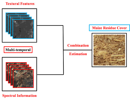
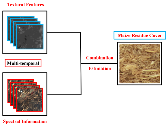
Estimation of Maize Residue Cover Using Landsat-8 OLI Image Spectral Information and Textural Features


Abstract
:
1. Introduction
2. Material and Methods
2.1. Study Area
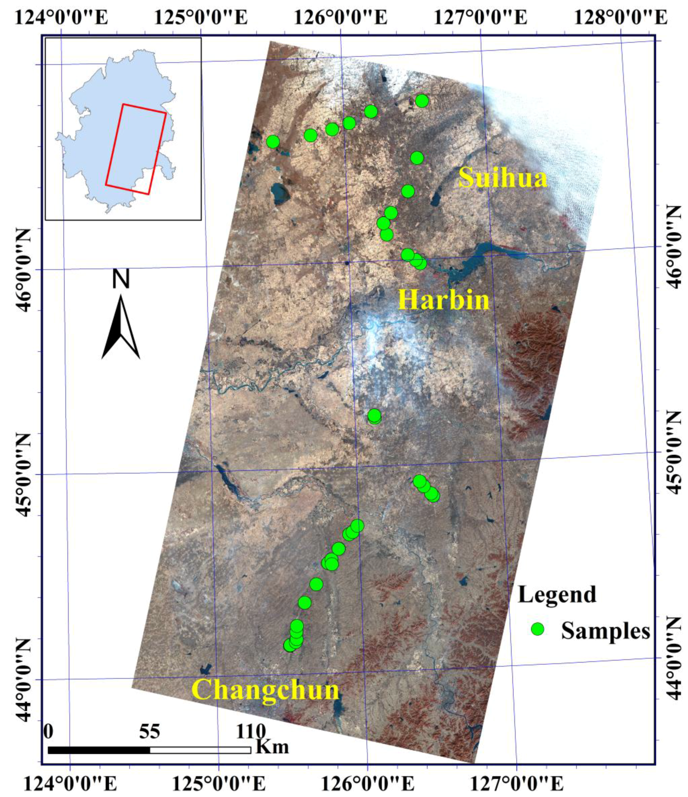
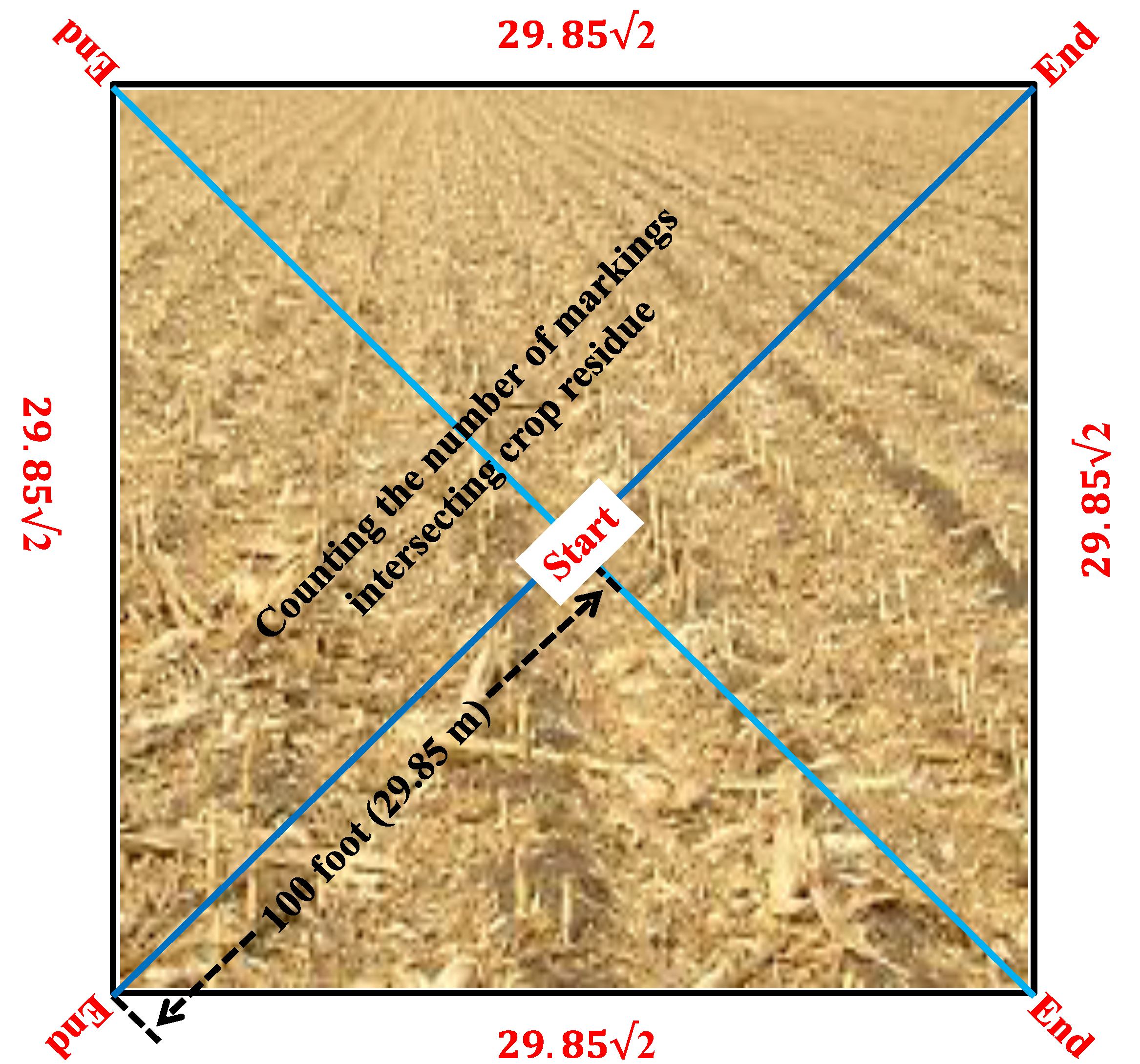
2.2. Field Measurements


| Dataset | Samples | Max | Min | Mean | Standard Deviation |
|---|---|---|---|---|---|
| Calibration dataset | 24 | 95.00 | 10.00 | 60.04 | 27.19 |
| Validation dataset | 12 | 89.00 | 10.90 | 59.60 | 27.67 |
2.3. Remote Sensing Data and Pre-Processing
2.4. Methods
2.4.1. Vegetation Indices
| Vegetation Index | Abbreviation | Formula | References |
|---|---|---|---|
| Simple tillage index | STI | B6/B7 | [16] |
| Normalized difference tillage index | NDTI | (B6 − B7)/(B6 + B7) | [16] |
| Modified crop residue cover | MCRC | (B6 − B3)/(B6 + B3) | [33] |
| Normalized difference index 5 | NDI5 | (B5 − B6)/(B5 + B6) | [15] |
| Normalized difference index 7 | NDI7 | (B5 − B7)/(B5 + B7) | [15] |
| Shortwave red normalized difference index | SRNDI | (B7 − B4)/(B7 + B4) | In this paper |
| Normalized difference senescent vegetation index | NDSVI | (B6 − B4)/(B6 + B4) | [17] |
2.4.2. Textural Features
2.4.3. Extraction of Maize Cultivation Area
2.4.4. Partial Least Squares Regression
2.5. Statistical Analysis
3. Results
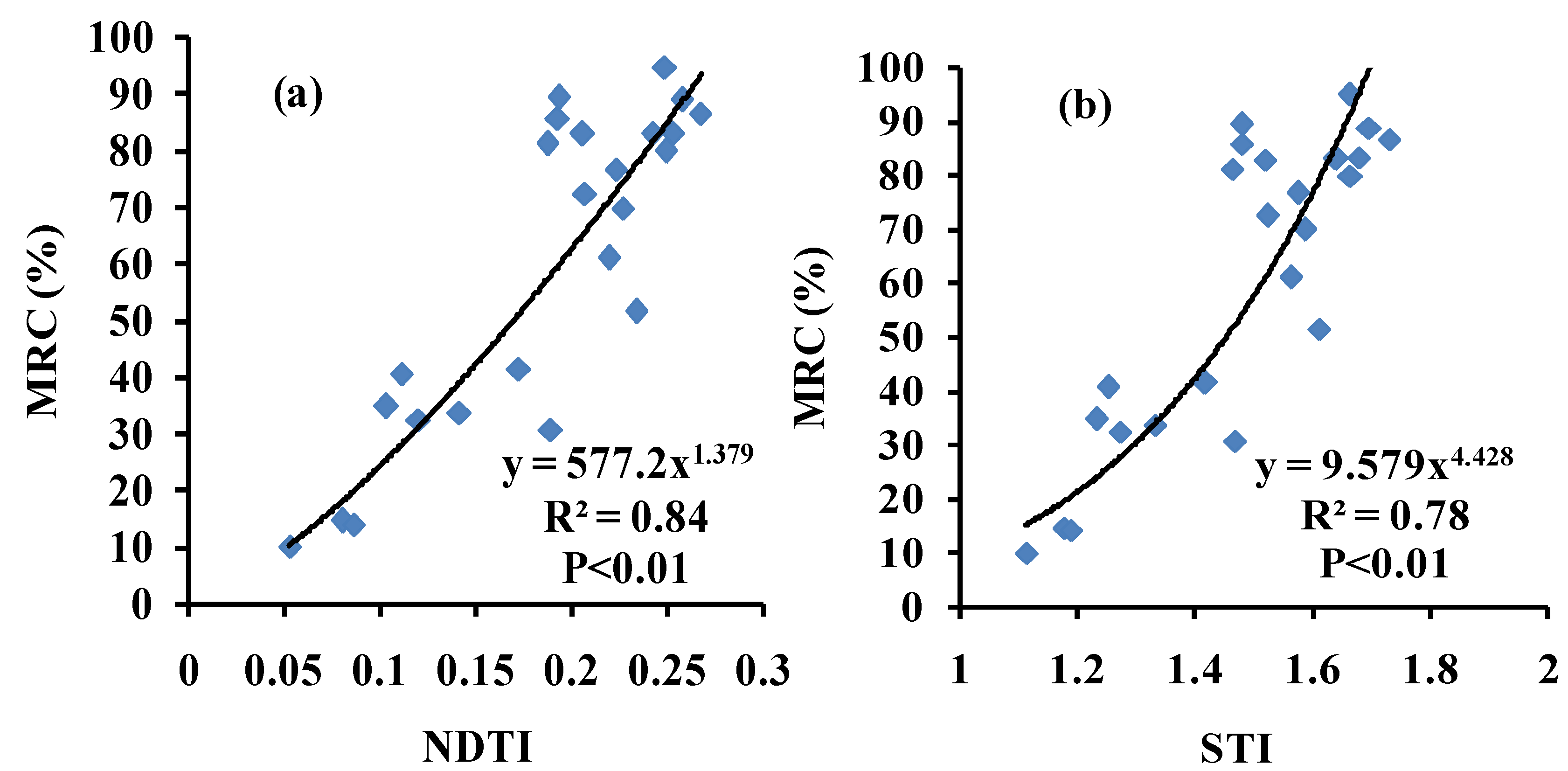
3.1. Relationship between Maize Residue Cover and Vegetation Indices
| Vegetation Index | Regression Equation | R2 | RMSE (%) |
|---|---|---|---|
| NDTI | y = 577.2x1.379 | 0.84 ** | 12.33 |
| STI | y = 9.579x4.428 | 0.78 ** | 13.71 |
| NDI7 | y = 40.15e3.538x | 0.72 ** | 14.63 |
| SRNDI | y = 101.7e−3.89x | 0.71 ** | 14.71 |
| NDI5 | y = 96.90e5.429x | 0.63 ** | 17.65 |
| NDSVI | y = 463.9e−6.24x | 0.57 ** | 18.56 |
| MCRC | y = 243.4x − 43.49 | 0.50 ** | 21.16 |

3.2. Relationship between Maize Residue Cover and Textural Features
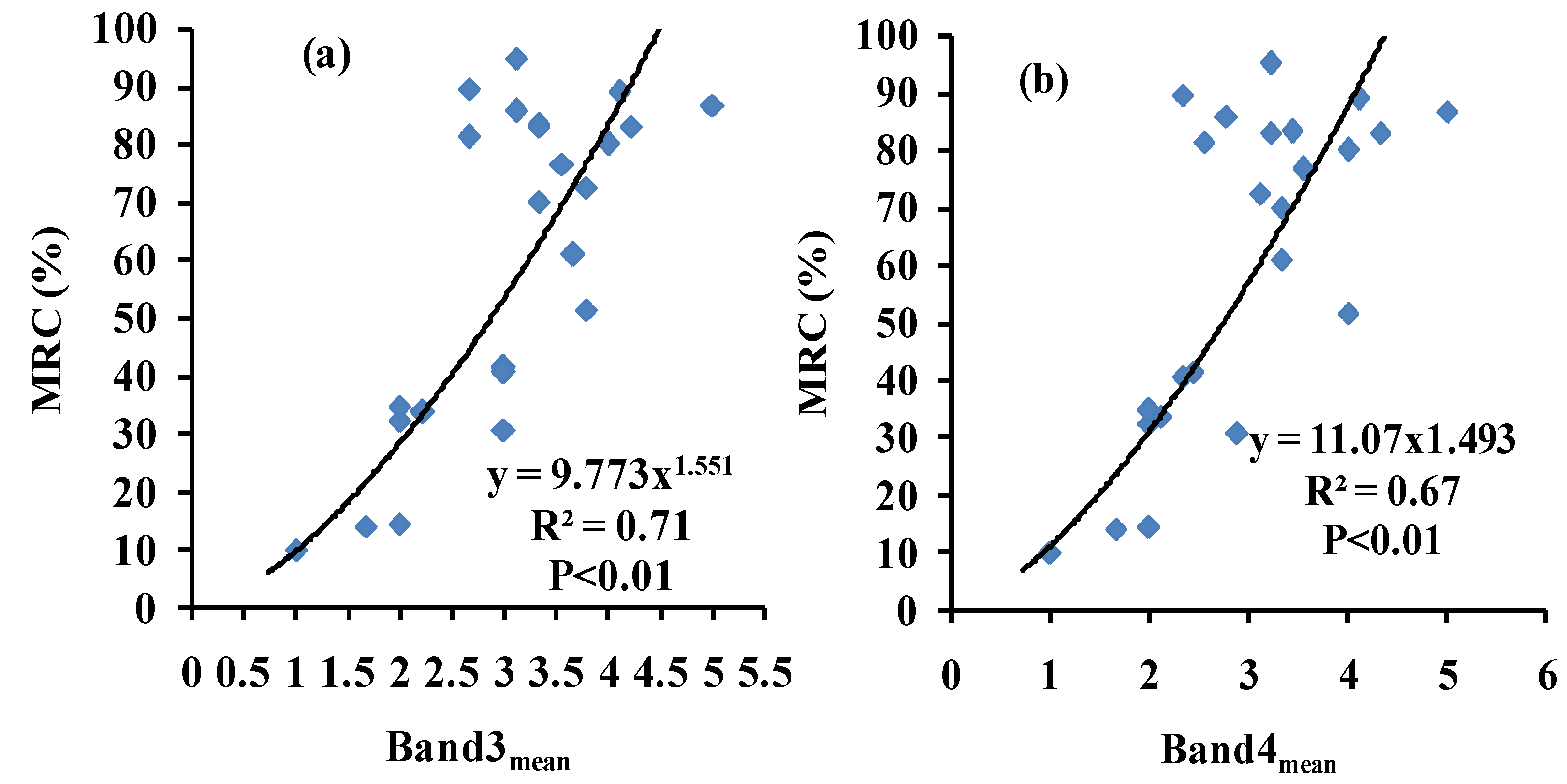
| Texture Feature Indicators | Regression Equation | R2 | RMSE (%) |
|---|---|---|---|
| Band3mean | y = 9.773x1.551 | 0.71 ** | 15.21 |
| Band4mean | y = 11.07x1.493 | 0.67 ** | 19.45 |
| Band5mean | y = 5.116x1.485 | 0.65 ** | 20.02 |
| Band2mean | y = 0.463x3.260 | 0.52 ** | 16.92 |
| Band6mean | y = 30.42x − 1004 | 0.43 ** | 21.72 |
| Band3correlation | y = −31.77x + 75.72 | 0.42 ** | 21.81 |
| Band3second moment | y = −27.9ln(x) + 39.94 | 0.37 ** | 23.31 |
| Band3entropy | y = 26.05x + 39.2 | 0.36 ** | 22.43 |
| Band3homogeneity | y = −101.8x + 146.4 | 0.26 * | 24.43 |
| Band3dissimilarity | y = 40.99x + 46.75 | 0.21 * | 26.35 |
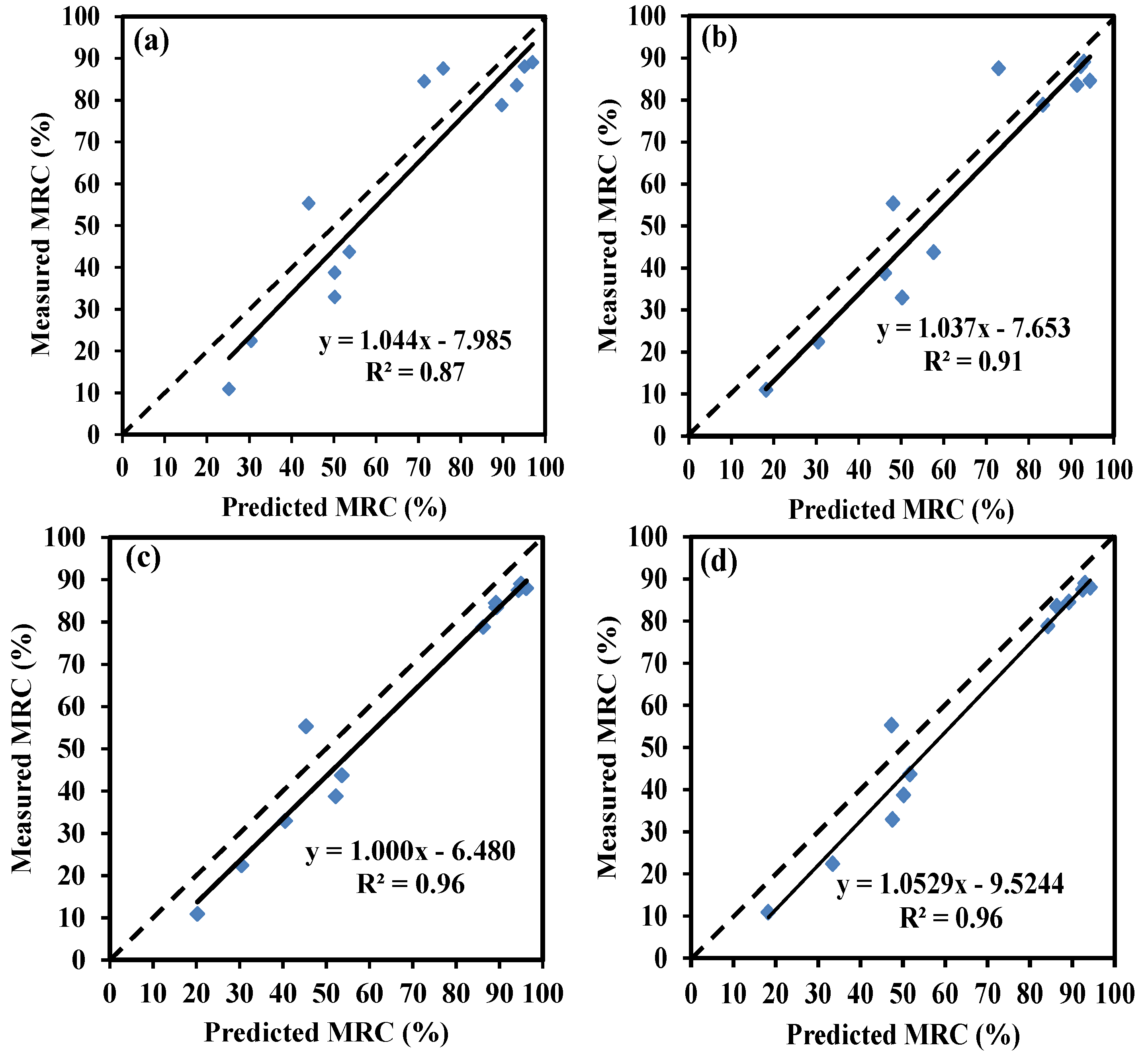
3.3. Estimating MRC via Partial Least Squares Regression (PLSR)

| Methods | Factor | R2 | RMSE (%) |
|---|---|---|---|
| Vegetation indices | NDTI, STI, NDI7, and SRNDI | 0.87 | 11.36 |
| STI, NDTI, MCRC, NDI5, NDI7, SRNDI, NDSVI | 0.88 | 11.34 | |
| Texture features | Band3mean, Band4mean, Band5mean | 0.83 | 12.32 |
| Band2mean, Band3mean, Band3homogeneity, Band3dissimilarity, Band3entropy, Band3second moment, Band3correlation, Band6mean | 0.90 | 9.82 | |
| Combination | NDI7, SINDI, STI, NDTI, Band3mean, Band4mean, Band5mean | 0.95 | 8.43 |
| STI, NDTI, MCRC, NDI5, NDI7, SRNDI, NDSVI, Band2mean, Band3mean, Band3homogeneity, Band3dissimilarity, Band3entropy, Band3second moment, Band3correlation, Band6mean | 0.96 | 8.11 |
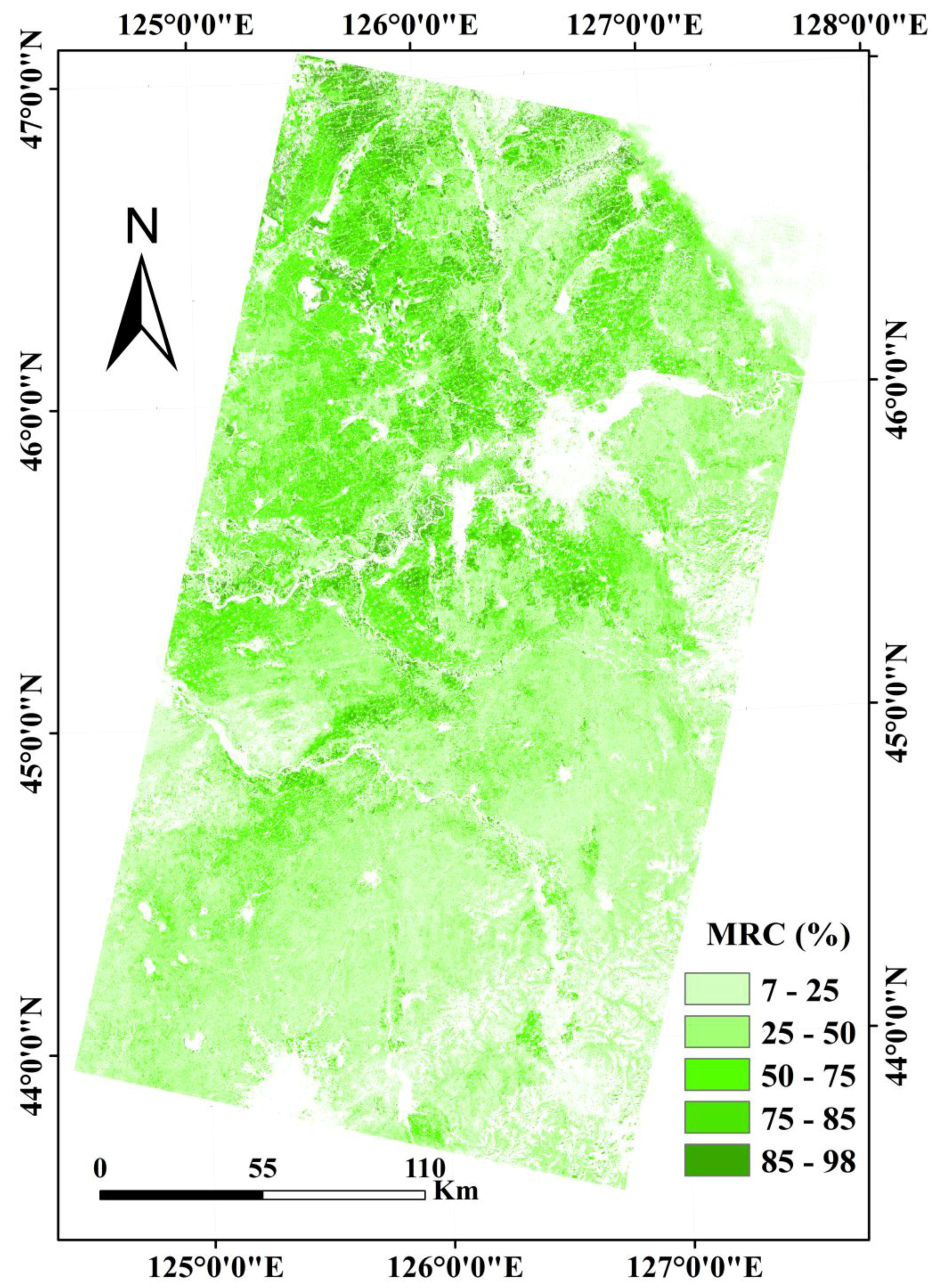
3.4. MRC Mapping

4. Discussion
5. Conclusions
Acknowledgments
Author Contributions
Conflicts of Interest
References
- Bannari, A.; Haboudane, D.; Bonn, F. Intérêt du moyen infrarouge pour la cartographie desrésidus de cultures. Can. J. Remote Sens. 2000, 26, 384–393. [Google Scholar] [CrossRef]
- Daughtry, C.S.; Hunt, E.R., Jr.; Doraiswamy, P.C.; McMurtrey, J.E. Remote sensing the spatial distribution of crop residues. Agron. J. 2005, 97, 864–871. [Google Scholar] [CrossRef]
- Tomer, M.D. Assessing the extent of conservation tillage in agricultural landscapes. Proc. SPIE 2012, 8531. [Google Scholar] [CrossRef]
- Bannari, A.; Staenz, K.; Champagne, C.; Khurshid, K.S. Spatial variability mapping of crop residue using Hyperion (EO-1) hyperspectral data. Remote Sens. 2015, 7, 8107–8127. [Google Scholar] [CrossRef]
- Aase, J.K.; Tanaka, D.L. Reflectance from four wheat residues cover densities as influenced by three soil backgrounds. Agron. J. 1991, 83, 753–757. [Google Scholar] [CrossRef]
- Ruane, J.; Sonnino, A.; Agostini, A. Bioenergy and the potential contribution of agricultural biotechnologies in developing countries. Biomass Bioenerg. 2010, 34, 1427–1439. [Google Scholar] [CrossRef]
- Pacheco, A.; McNairn, H. Evaluating multispectral remote sensing and spectral unmixing analysis for crop residue mapping. Remote Sens. Environ. 2010, 114, 2219–2228. [Google Scholar] [CrossRef]
- Daughtry, C.S. Discriminating crop residues from soil by shortwave infrared reflectance. Agron. J. 2001, 93, 125–131. [Google Scholar] [CrossRef]
- Daughtry, C.S.T.; Hunt, E.R.; McMurtrey, J.E. Assessing crop residue cover using shortwave infrared reflectance. Remote Sens. Environ. 2004, 90, 126–134. [Google Scholar] [CrossRef]
- Bannari, A.; Pacheco, A.; Staenz, K.; McNairn, H.; Omari, K. Estimating and mapping crop residues cover on agricultural lands using hyperspectral and IKONOS data. Remote Sens. Environ. 2006, 104, 447–459. [Google Scholar] [CrossRef]
- Galloza, M.S.; Crawford, M.M.; Heathman, G.C. Crop residue modeling and mapping using Landsat, ALI, Hyperion and airborne remote sensing data. IEEE JSTAR 2013, 6, 446–456. [Google Scholar]
- Gausman, H.W.; Gerbermann, A.H.; Wiegand, C.L.; Leamer, R.W.; Rodriguez, R.R.; Noriega, J.R. Reflectance differences between crop residues and bare soils. Soil Sci. Soc. Am. J. 1975, 39, 752–755. [Google Scholar] [CrossRef]
- Daughtry, C.S.; Hunt, E.R. Mitigating the effects of soil and residue water contents on remotely sensed estimates of crop residue cover. Remote Sens. Environ. 2008, 112, 1647–1657. [Google Scholar] [CrossRef]
- Serbin, G.; Hunt, E.R.; Daughtry, C.S.; McCarty, G.W.; Doraiswamy, P.C. An improved ASTER index for remote sensing of crop residue. Remote Sens. 2009, 1, 971–991. [Google Scholar] [CrossRef]
- McNairn, H.; Protz, R. Mapping corn residue cover on agricultural fields in Oxford County, Ontario, using Thematic Mapper. Can. J. Remote Sens. 1993, 19, 152–159. [Google Scholar] [CrossRef]
- Van Deventer, A.P.; Ward, A.D.; Gowda, P.H.; Lyon, J.G. Using thematic mapper data to identify contrasting soil plains and tillage practices. Photogramm. Eng. Remote Sens. 1997, 63, 87–93. [Google Scholar]
- Qi, J.; Marsett, R.; Heilman, P.; Biedenbender, S.; Goodrich, D. Ranges improves satellite based information and land cover assessments in Southwest United States. Eos Trans. Am. Geophys. Union 2002, 83, 601–606. [Google Scholar] [CrossRef]
- Zheng, B.; Campbell, J.B.; de Beurs, K.M. Remote sensing of crop residue cover using multi-temporal Landsat imagery. Remote Sens. Environ. 2012, 117, 177–183. [Google Scholar] [CrossRef]
- Zheng, B.; Campbell, J.B.; Shao, Y.; Wynne, R.H. Broad-scale monitoring of tillage practices using sequential Landsat imagery. Soil Sci. Soc. Am. J. 2013, 77, 1755–1764. [Google Scholar] [CrossRef]
- Bocco, M.; Sayago, S.; Willington, E. Neural network and crop residue index multiband models for estimating crop residue cover from Landsat TM and ETM+ images. Int. J. Remote Sens. 2014, 35, 3651–3663. [Google Scholar] [CrossRef]
- Levine, M. Vision in Man and Machine; McGraw-Hill: New York, NY, USA, 1985. [Google Scholar]
- Wood, E.M.; Pidgeon, A.M.; Radeloff, V.C.; Keuler, N.S. Image texture as a remotely sensed measure of vegetation structure. Remote Sens. Environ. 2012, 121, 516–526. [Google Scholar] [CrossRef]
- Beguet, B.; Guyon, D.; Boukir, S.; Chehata, N. Automated retrieval of forest structure variables based on multi-scale texture analysis of VHR satellite imagery. ISPRS J. Photogramm. Remote Sens. 2014, 96, 164–178. [Google Scholar] [CrossRef]
- Nichol, J.E.; Sarker, M.L.R. Improved Biomass Estimation Using the Texture Parameters of Two High-Resolution Optical Sensors. IEEE Trans. Geosci. Remote Sens. 2011, 49, 930–948. [Google Scholar] [CrossRef]
- Darvishzadeh, R.; Skidmore, A.; Schlerf, M.; Atzberger, C.; Corsi, F.; Cho, M. LAI and chlorophyll estimation for a heterogeneous grassland using hyperspectral measurements. ISPRS J. Photogramm. Rem. Sens. 2008, 63, 409–426. [Google Scholar] [CrossRef]
- Li, X.; Zhang, Y.; Bao, Y.; Luo, J.; Jin, X.; Xu, X.; Song, X.; Yang, G. Exploring the best hyperspectral features for LAI estimation using Partial Least Squares Regression. Remote Sens. 2014, 6, 6221–6241. [Google Scholar] [CrossRef]
- Mutanga, O.; Adam, E.; Adjorlolo, C.; Abdel-Rahman, E.M. Evaluating the robustness of models developed from field spectral data in predicting African grass foliar nitrogen concentration using WorldView-2 image as an independent test dataset. Int. J. Appl. Earth Observ. 2015, 34, 178–187. [Google Scholar] [CrossRef]
- Oumar, Z.; Mutanga, O.; Ismail, R. Predicting Thaumastocoris peregrinus damage using narrow band normalized indices and hyperspectral indices using field spectra resampled to the Hyperion sensor. Int. J. Appl. Earth Observ. 2013, 21, 113–121. [Google Scholar] [CrossRef]
- Thenkabail, P.S.; Enclona, E.A.; Ashton, M.S.; van der Meer, B. Accuracy assessments of hyperspectral waveband performance for vegetation analysis applications. Remote Sens. Environ. 2004, 91, 354–376. [Google Scholar] [CrossRef]
- Ren, C.Y.; Zhang, C.H.; Wang, Z.M.; Zhang, B. Organic Carbon Storage and Sequestration Potentialin Cropland Surface Soils of Songne plain mazie belt. J. Nat. Resour. 2013, 28, 596–607. (In Chinese) [Google Scholar]
- Morrison, J.E.; Huang, C.H.; Lightle, D.T.; Daughtry, C.S.T. Residue measurement techniques. J. Soil Water Conserv. 1993, 48, 478–483. [Google Scholar]
- NRCS. Farming with Crop Residue Brochure. 1992. Available online: http://www.il.nrcs.usda.gov/news/publications/brochures/farmcropres/FarmCropRes-broc.html (accessed on 15 March 2010). [Google Scholar]
- Sullivan, D.G.; Truman, C.C.; Schomberg, H.H.; Endale, D.M.; Strickland, T.C. Evaluating techniques for determining tillage regime in the Southeastern Coastal Plain and Piedmont. Agron. J. 2006, 98, 1236–1246. [Google Scholar] [CrossRef]
- Richards, J.A. Remote Sensing Digital Image Analysis; Springer-Verlag: Berlin, Germany, 1999. [Google Scholar]
- Abdi, H. Partial Least Square Regression (PLS Regression). In Encyclopedia of Measurement and Statistics; Salkind, N., Ed.; SAGE: Thousand Oaks, CA, USA, 2003; pp. 792–795. [Google Scholar]
- Hansen, P.M.; Schjoerring, J.K. Reflectance measurement of canopy biomass and nitrogen status in wheat crops using normalized difference vegetation indices and partial least squares regression. Remote Sens. Environ. 2003, 86, 542–553. [Google Scholar] [CrossRef]
- Jin, X.L.; Xu, X.G.; Song, X.Y.; Li, Z.H.; Wang, J.H.; Guo, W.S. Estimation of leaf water content in winter wheat using grey relational analysis-partial least squares modeling with hyperspectral data. Agron. J. 2013, 105, 1385–1392. [Google Scholar] [CrossRef]
- Wang, B.S. Field-Experiment and Statistic-Method; Chinese Agriculture Press: Beijing, China, 2002. [Google Scholar]
- Murray, I.; Williams, P.C. Chemical principles of near-infrared technology. In Near-Infrared Technology in the Agricultural and Food Industries; Williams, P., Norris, K., Eds.; American Association of Cereal Chemists: St. Paul, MN, USA, 1988; pp. 17–34. [Google Scholar]
- Annea, N.J.P.; Abd-Elrahman, A.H.; Lewis, D.B.; Hewitta, N.A. Modeling soil parameters using hyperspectral image reflectance in subtropical coastal wetlands. Int. J. Appl. Earth Observ. 2014, 33, 47–56. [Google Scholar] [CrossRef]
- Franceschini, M.H.D.; Demattêa, J.A.M.; da Silva Terra, F.; Vicente, L.E.; Bartholomeus, H.; de Souza Filho, C.R. Prediction of soil properties using imaging spectroscopy: Considering fractional vegetation cover to improve accuracy. Int. J. Appl. Earth Observ. 2015, 38, 358–370. [Google Scholar] [CrossRef]
- Jia, M.M.; Zhang, Y.Z.; Wang, Z.M.; Song, K.S.; Ren, C.Y. Mapping the distribution of mangrove species in the Core Zone of Mai Po Marshes Nature Reserve, Hong Kong, using hyperspectral data and high-resolution data. Int. J. Appl. Earth Observ. 2014, 33, 226–231. [Google Scholar] [CrossRef]
- Lagacherie, P.; Sneep, A.R.; Gomez, C.; Bacha, S.; Coulouma, G.; Hamrouni, M.H.; Mekki, I. Combining Vis-NIR hyperspectral imagery and legacy measured soil profiles to map subsurface soil properties in a Mediterranean area (Cap-Bon, Tunisia). Geoderma 2013, 209–210, 168–176. [Google Scholar] [CrossRef]
- Liu, S.H.; An, N.N.; Yang, J.J.; Dong, S.K.; Wang, C.; Yin, Y.J. Prediction of soil organic matter variability associated with different land use types in mountainous landscape in southwestern Yunnan province, China. Catena 2015, 133, 137–144. [Google Scholar] [CrossRef]
- Peng, X.; Shi, T.; Song, A.; Chen, Y.; Gao, W. Estimating soil organic carbon using VIS/NIR spectroscopy with SVMR and SPA methods. Remote Sens. 2014, 6, 2699–2717. [Google Scholar] [CrossRef]
- Wanjura, D.F.; Bilbro, J.D. Ground cover and weathering effects on reflectance of three crop residues. Agron. J. 1986, 78, 694–698. [Google Scholar] [CrossRef]
- Daughtry, C.S.; Doraiswamym, P.; Hunt, E.R.; Stern, A.; McMurtrey, J.E.; Prueger, J. Remote sensing of crop residue cover and soil tillage intensity. Soil Tillage Res. 2006, 91, 101–108. [Google Scholar] [CrossRef]
- Berberoglu, S.; Lloyd, C.D.; Atkinson, P.M.; Curran, P.J. The integration of spectral and textural information using neural networks for land cover mapping in the Mediterranean. Comput. Geosci. 2000, 26, 385–396. [Google Scholar] [CrossRef]
- Lu, D. The potential and challenge of remote sensing-based biomass estimation. Int. J. Remote Sens. 2006, 27, 1297–1328. [Google Scholar] [CrossRef]
- Zhou, J.; Zhao, Z.; Zhao, J.; Zhao, Q.; Wang, F.; Wang, H. A comparison of three methods for estimating the LAI of black locust. Int. J. Remote Sens. 2014, 35, 171–188. [Google Scholar] [CrossRef]
- Kelsey, K.; Neff, J. Estimates of aboveground biomass from texture analysis of Landsat imagery. Remote Sens. 2014, 6, 6407–6422. [Google Scholar] [CrossRef]
- Fourty, T.; Baret, F. Vegetation water and dry matter contents estimated from top-of-the-atmosphere reflectance data: A simulation. Remote Sens. Environ. 1997, 61, 34–45. [Google Scholar] [CrossRef]
© 2015 by the authors; licensee MDPI, Basel, Switzerland. This article is an open access article distributed under the terms and conditions of the Creative Commons Attribution license (http://creativecommons.org/licenses/by/4.0/).
Share and Cite
Jin, X.; Ma, J.; Wen, Z.; Song, K. Estimation of Maize Residue Cover Using Landsat-8 OLI Image Spectral Information and Textural Features. Remote Sens. 2015, 7, 14559-14575. https://doi.org/10.3390/rs71114559
Jin X, Ma J, Wen Z, Song K. Estimation of Maize Residue Cover Using Landsat-8 OLI Image Spectral Information and Textural Features. Remote Sensing. 2015; 7(11):14559-14575. https://doi.org/10.3390/rs71114559
Chicago/Turabian StyleJin, Xiuliang, Jianhang Ma, Zhidan Wen, and Kaishan Song. 2015. "Estimation of Maize Residue Cover Using Landsat-8 OLI Image Spectral Information and Textural Features" Remote Sensing 7, no. 11: 14559-14575. https://doi.org/10.3390/rs71114559
APA StyleJin, X., Ma, J., Wen, Z., & Song, K. (2015). Estimation of Maize Residue Cover Using Landsat-8 OLI Image Spectral Information and Textural Features. Remote Sensing, 7(11), 14559-14575. https://doi.org/10.3390/rs71114559