
Spatiotemporal Variation in Mangrove Chlorophyll Concentration Using Landsat 8

 ,
, 
Abstract
:
1. Introduction
2. Methods
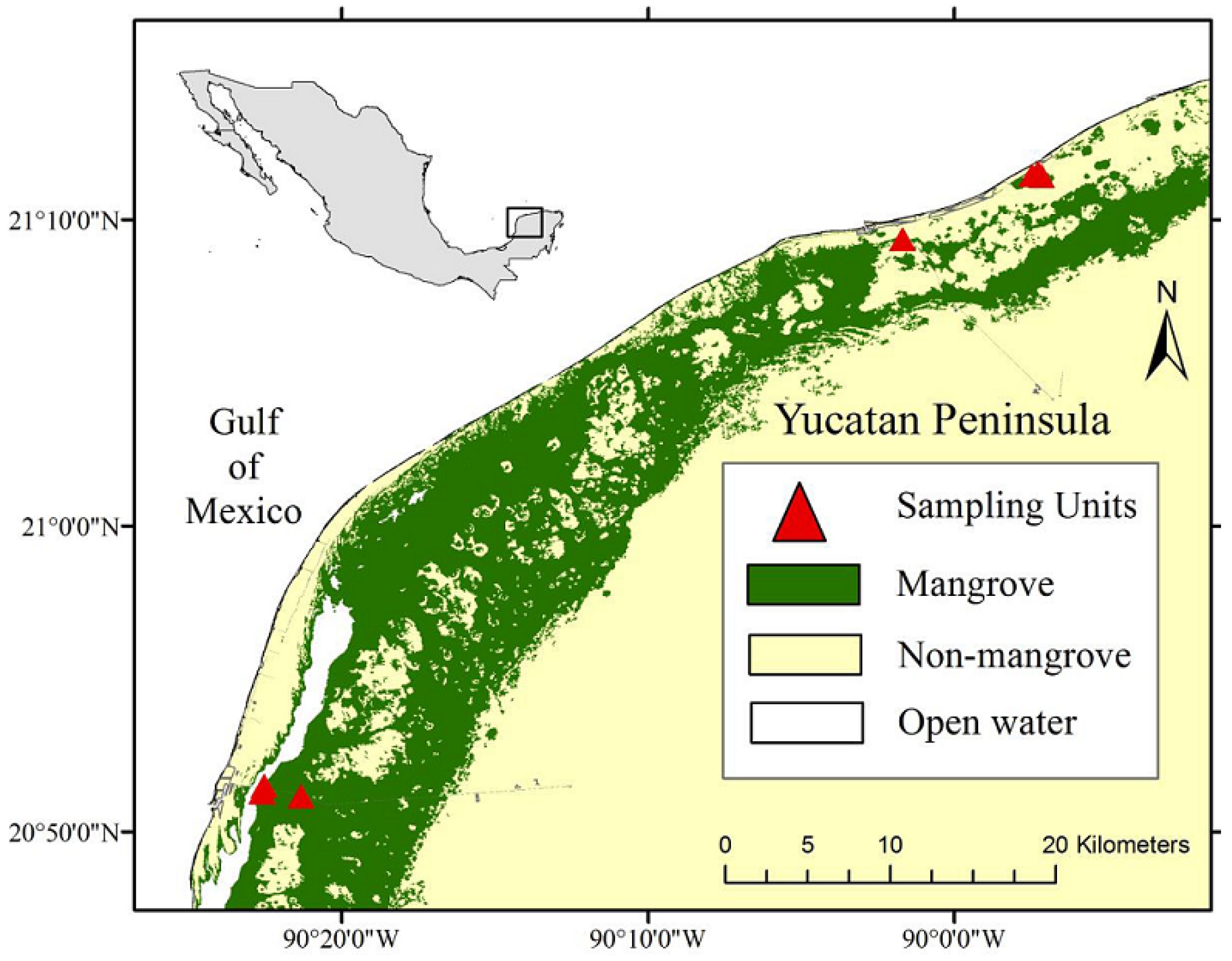
2.1. Study Area
2.2. Data Acquisition
Ground Data Collection
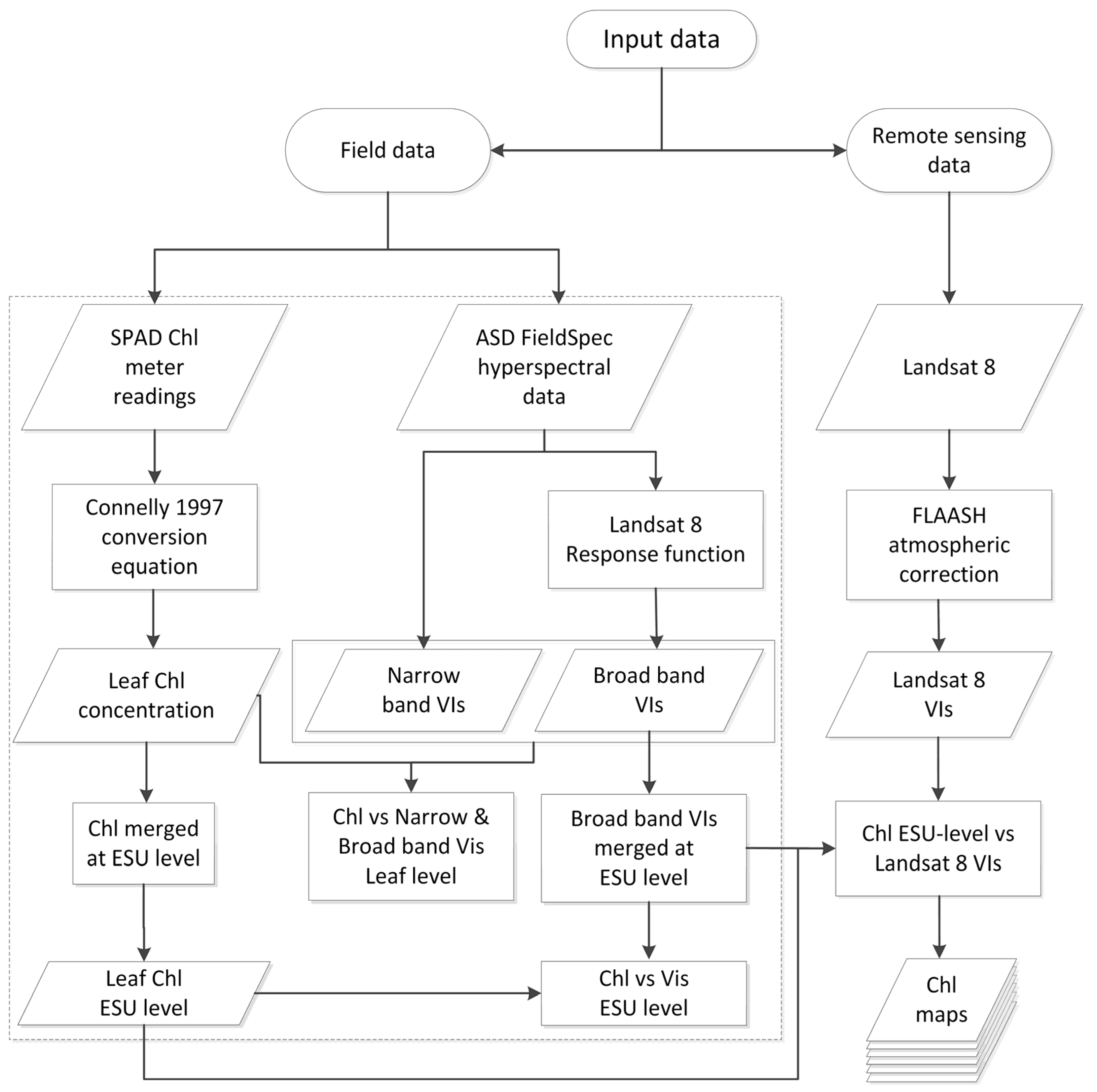
2.3. Ground Data Processing
2.3.1. SPAD Calibration

| Vegetation Index | Abbreviation | Formula | Reference |
|---|---|---|---|
| Simple Ratio Index680 | SR680 | [61] | |
| Simple Ratio Index750 | SR750 | [62] | |
| Normalized Difference Vegetation Index680 | NDVI680 | [63] | |
| Normalized Difference Vegetation Index705 | NDVI705 | [62] | |
| Modified Red Edge Simple Ratio Index | mSR705 | [45] | |
| Modified Normalized Difference Vegetation Index | mND705 | [45] | |
| MERIS Terrestrial Chlorophyll Index | MTCI | [40] | |
| Vogelmann Red Edge Index 1 | VOG1 | [64] | |
| Vogelmann Red Edge Index 2 | VOG2 | [65] | |
| Vogelmann Red Edge Index 3 | VOG3 | [65] | |
| Photochemical Reflectance Index | PRI | [66] | |
| Transformed Chlorophyll Absorption Ratio Index | TCARI | [67] | |
| Modified Chlorophyll Absorption Index | mCARI705 | [68] | |
| Green Normalized Difference Vegetation Index | NDVI green | [69] | |
| Simple Ratio | Simple Ratio | [61] | |
| Green Chlorophyll Index | CI green | [44] | |
| Normalized Difference Vegetation Index | NDVI | [63] | |
| Enhanced Vegetation Index | EVI1 | [70] | |
| Enhanced Vegetation Index 2 | EVI2 | [71] | |
| Wide Dynamic Rage Vegetation Index | WDRVI | [72] | |
| Green Wide Dynamic Range Vegetation Index | WDRVI green | [73] |
2.3.2. Hyperspectral Data Processing
2.4. Satellite Sensor Data Processing
Statistical Analysis
3. Results
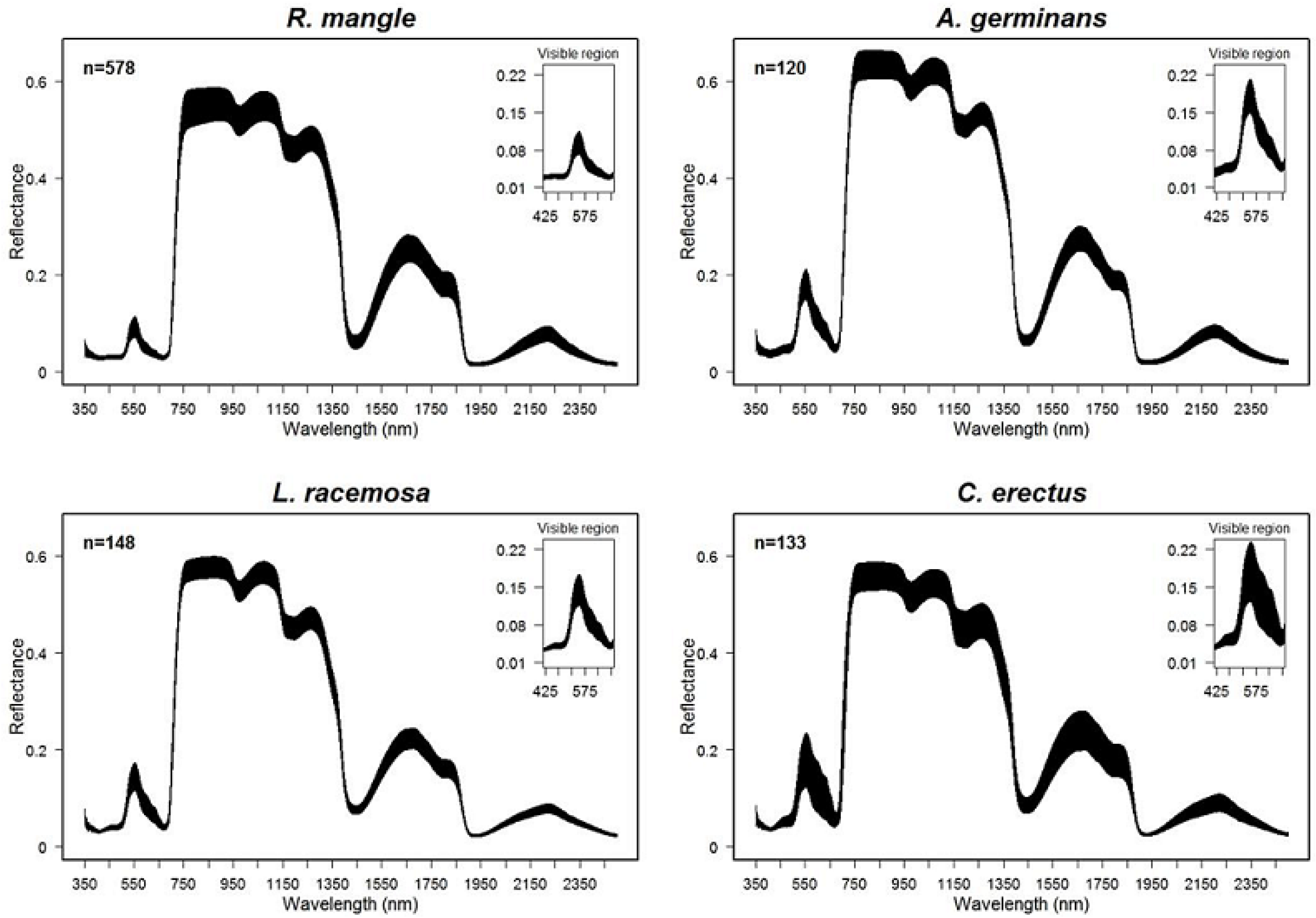
3.1. Spectral Variation among Species

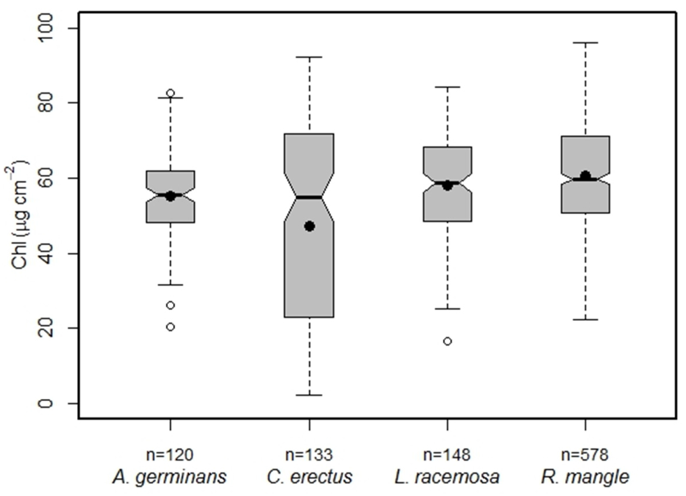
3.2. Mangrove Species CC

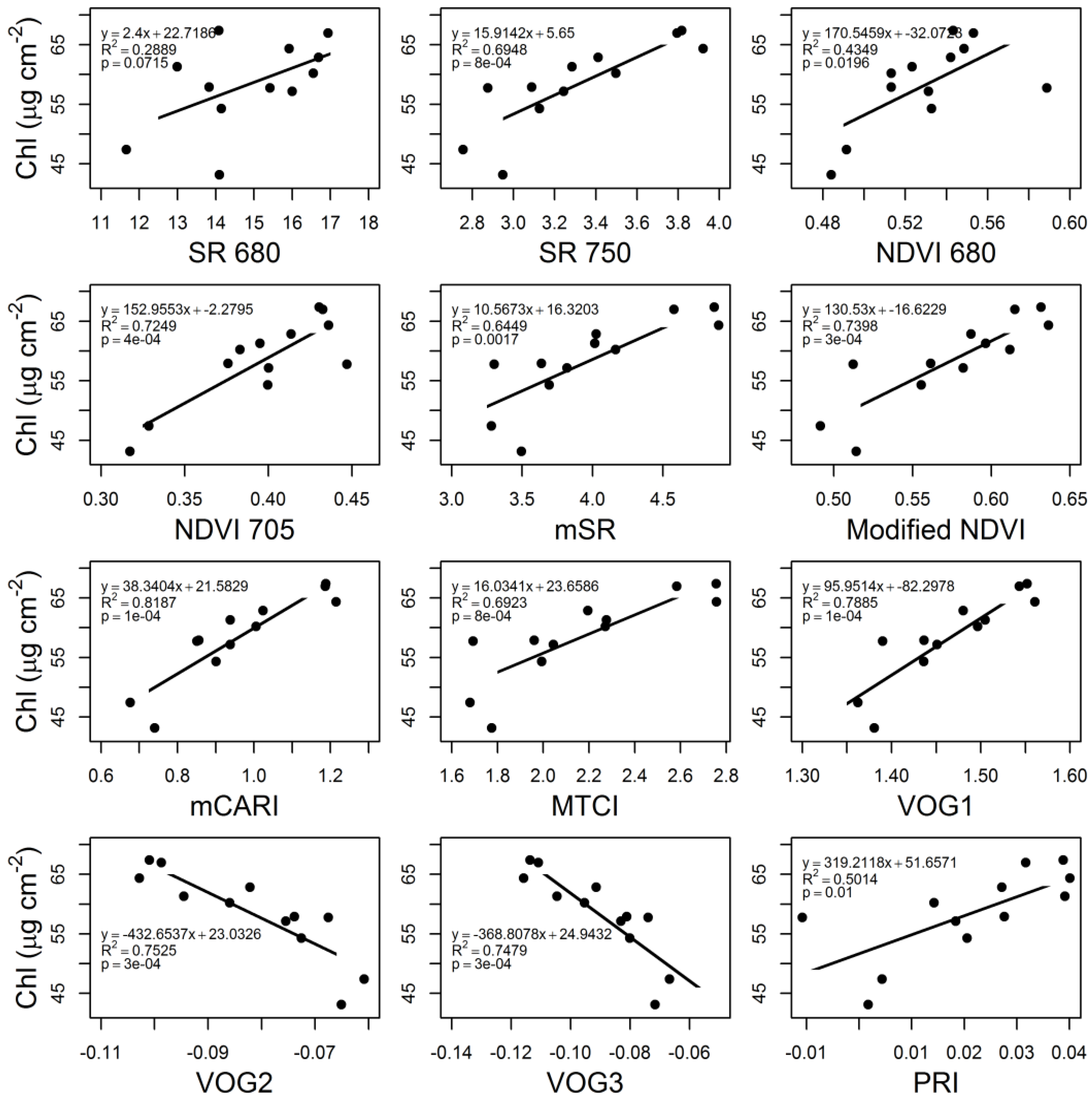
3.3. Performance of VIs
| VI | Intercept | Slope | R2 | RMSE | Signif. |
|---|---|---|---|---|---|
| VOG2 | 20.382 | –449.057 | 0.588 | 11.3 | *** |
| VOG1 | −77.714 | 91.798 | 0.587 | 11.3 | *** |
| VOG3 | 22.558 | −379.752 | 0.582 | 11.4 | *** |
| MTCI | 22.817 | 15.554 | 0.564 | 11.7 | *** |
| mND705 | −7.524 | 112.029 | 0.551 | 11.8 | *** |
| mSR705 | 16.172 | 10.088 | 0.530 | 12.1 | *** |
| mCARI705 | 22.597 | 35.201 | 0.528 | 12.1 | *** |
| SR750 | 9.051 | 14.264 | 0.514 | 12.3 | *** |
| TCARI | 82.556 | −103.717 | 0.457 | 13.0 | *** |
| WDRVI green | 15.381 | 65.250 | 0.450 | 13.1 | *** |
| NDVI green | 2.228 | 92.202 | 0.446 | 13.2 | *** |
| CI green | 30.693 | 7.828 | 0.432 | 13.3 | *** |
| NDVI | −40.481 | 120.412 | 0.281 | 15.0 | *** |
| WDRVI | 27.422 | 60.234 | 0.274 | 15.1 | *** |
| SR | 30.901 | 2.438 | 0.217 | 15.6 | *** |
| EVI2 | −30.779 | 228.633 | 0.203 | 15.8 | *** |
| EVI1 | −34.546 | 221.288 | 0.198 | 15.8 | *** |
| NDVI705 | 10.544 | 116.844 | 0.185 | 16.0 | *** |
| SR680 | 32.193 | 1.614 | 0.116 | 16.6 | *** |
| NDVI680 | 40.587 | 30.073 | 0.006 | 17.6 | * |

| VI | Intercept | Slope | R2 | RMSE | Signif. |
|---|---|---|---|---|---|
| VOG2 | 18.188 | −451.792 | 0.693 | 5.7 | *** |
| VOG3 | 21.345 | −373.644 | 0.688 | 5.7 | *** |
| VOG1 | −87.574 | 96.967 | 0.672 | 5.8 | *** |
| mND705 | −42.674 | 163.958 | 0.672 | 5.8 | *** |
| MTCI | 22.359 | 15.054 | 0.670 | 5.9 | *** |
| mSR705 | 14.913 | 9.963 | 0.650 | 6.0 | *** |
| SR750 | 4.131 | 15.024 | 0.621 | 6.3 | *** |
| NDVIgreen | −54.493 | 174.230 | 0.609 | 6.4 | *** |
| WDRVIgreen | −13.384 | 100.923 | 0.607 | 6.4 | *** |
| CIgreen | 24.163 | 8.929 | 0.584 | 6.6 | *** |
| mCARI705 | 23.182 | 33.436 | 0.582 | 6.6 | *** |
| TCARI | 93.665 | −174.992 | 0.577 | 6.6 | *** |
| NDVI705 | 29.339 | 81.311 | 0.114 | 9.6 | *** |
| WDRVI | 31.829 | 51.978 | 0.056 | 10.0 | *** |
| SR | 44.576 | 1.352 | 0.055 | 10.0 | *** |
| NDVI | −43.281 | 123.583 | 0.055 | 10.0 | *** |
| EVI1 | 15.393 | 110.420 | 0.043 | 10.0 | *** |
| EVI2 | 20.601 | 104.767 | 0.037 | 10.1 | *** |
| NDVI680 | 44.377 | 33.138 | 0.011 | 10.2 | ** |
| SR680 | 60.735 | 0.049 | 0.000 | 10.2 | ns |
| VI | Intercept | Slope | R2 | RMSE | Signif. |
|---|---|---|---|---|---|
| VOG2 | 26.277 | −274.101 | 0.881 | 0.6 | *** |
| VOG3 | 27.114 | −238.934 | 0.880 | 0.6 | *** |
| MTCI | 26.178 | 10.039 | 0.866 | 0.6 | *** |
| VOG1 | −26.703 | 50.467 | 0.865 | 0.6 | *** |
| mSR705 | 19.105 | 7.395 | 0.852 | 0.7 | *** |
| CI green | 27.373 | 6.728 | 0.841 | 0.7 | *** |
| SR750 | 15.436 | 9.852 | 0.838 | 0.7 | *** |
| TCARI | 60.562 | −57.535 | 0.835 | 0.7 | *** |
| mND705 | 12.596 | 58.631 | 0.830 | 0.7 | *** |
| WDRVI green | 21.085 | 41.491 | 0.830 | 0.7 | *** |
| NDVI green | 14.663 | 53.726 | 0.809 | 0.8 | *** |
| mCARI705 | 26.561 | 21.353 | 0.804 | 0.8 | *** |
| WDRVI | 24.994 | 41.655 | 0.545 | 1.2 | *** |
| SR | 23.427 | 2.278 | 0.541 | 1.2 | *** |
| NDVI | −22.222 | 82.947 | 0.536 | 1.2 | *** |
| EVI1 | −13.213 | 135.008 | 0.422 | 1.4 | *** |
| EVI2 | −10.006 | 138.282 | 0.420 | 1.4 | *** |
| NDVI705 | 16.729 | 65.825 | 0.384 | 1.4 | *** |
| SR680 | 29.778 | 0.964 | 0.139 | 1.7 | *** |
| NDVI680 | 19.155 | 43.457 | 0.059 | 1.7 | ** |
| VI | Intercept | Slope | R2 | RMSE | Signif. |
|---|---|---|---|---|---|
| VOG2 | 29.348 | −309.760 | 0.639 | 0.9 | *** |
| VOG3 | 30.320 | −273.024 | 0.634 | 0.9 | *** |
| mCARI705 | 28.267 | 29.045 | 0.627 | 0.9 | *** |
| MTCI | 28.543 | 14.332 | 0.594 | 1.0 | *** |
| mND705 | 12.727 | 77.113 | 0.590 | 1.0 | *** |
| VOG1 | −34.331 | 61.339 | 0.589 | 1.0 | *** |
| mSR705 | 17.873 | 11.066 | 0.579 | 1.0 | *** |
| SR750 | 16.139 | 13.104 | 0.523 | 1.0 | *** |
| EVI1 | −17.632 | 152.880 | 0.492 | 1.0 | *** |
| EVI2 | −16.545 | 164.050 | 0.452 | 1.1 | *** |
| NDVI green | 26.849 | 47.782 | 0.384 | 1.2 | *** |
| WDRVI green | 32.141 | 38.064 | 0.372 | 1.2 | *** |
| TCARI | 66.330 | −42.785 | 0.362 | 1.2 | *** |
| CI green | 37.155 | 6.625 | 0.346 | 1.2 | *** |
| NDVI705 | 21.378 | 59.379 | 0.258 | 1.3 | *** |
| NDVI | 14.489 | 45.855 | 0.188 | 1.3 | *** |
| WDRVI | 40.738 | 22.664 | 0.175 | 1.3 | *** |
| NDVI680 | 13.451 | 58.514 | 0.136 | 1.4 | ** |
| SR | 40.683 | 1.125 | 0.127 | 1.4 | ** |
| SR680 | 39.332 | 0.765 | 0.077 | 1.4 | * |
| VI | Intercept | Slope | R2 | RMSE | Signif. |
|---|---|---|---|---|---|
| VOG2 | 4.968 | −1013.500 | 0.834 | 5.0 | *** |
| VOG3 | 6.924 | −895.743 | 0.830 | 5.0 | *** |
| VOG1 | −182.561 | 181.758 | 0.817 | 5.2 | *** |
| mCARI705 | 6.077 | 84.213 | 0.810 | 5.3 | *** |
| mND705 | −26.193 | 188.601 | 0.794 | 5.5 | *** |
| EVI2 | −146.001 | 602.331 | 0.794 | 5.5 | *** |
| EVI1 | −144.589 | 545.121 | 0.783 | 5.7 | *** |
| MTCI | 4.549 | 36.791 | 0.779 | 5.7 | *** |
| NDVI705 | −58.082 | 335.829 | 0.776 | 5.8 | *** |
| SR750 | −34.070 | 37.251 | 0.775 | 5.8 | *** |
| mSR705 | −20.928 | 27.366 | 0.768 | 5.9 | *** |
| SR680 | −64.088 | 12.103 | 0.755 | 6.0 | *** |
| NDVI green | −23.472 | 188.194 | 0.735 | 6.3 | *** |
| WDRVI green | −7.665 | 157.046 | 0.726 | 6.4 | *** |
| WDRVI | 19.586 | 143.564 | 0.711 | 6.6 | *** |
| NDVI | −116.197 | 250.425 | 0.705 | 6.6 | *** |
| CI green | 7.468 | 28.715 | 0.698 | 6.7 | *** |
| TCARI | 130.880 | −201.672 | 0.686 | 6.8 | *** |
| SR | −13.847 | 11.322 | 0.685 | 6.8 | *** |
| NDVI680 | −253.313 | 605.497 | 0.501 | 8.6 | *** |
3.4. VIs and CC at the ESU Level

3.5. Chl Concentration and Landsat 8 VIs

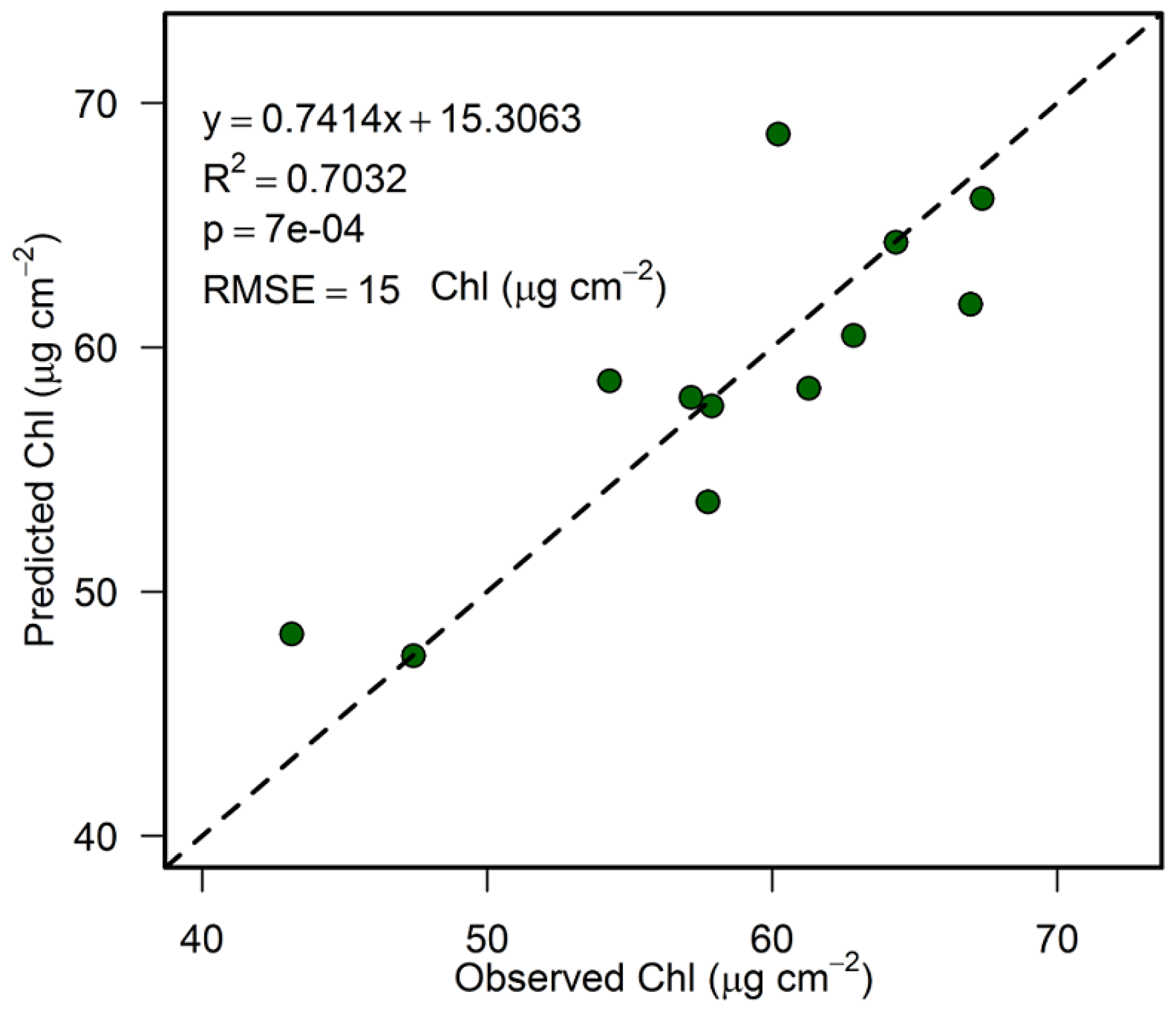
3.6. Accuracy Assessment

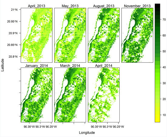
3.7. Spatial Variation of Chlorophyll Concentration across the Study Site


4. Discussion
4.1. Spectral Signature and Chl Concentration
4.2. Chl Concentration and Narrow Band Vegetation Indices
4.3. Chl Concentration and Broad Band Vegetation Indices Performance from Leaf to ESU Level
4.4. Chl Map
5. Conclusions
Supplementary Files
Supplementary File 1Acknowledgments
Author Contributions
Conflicts of Interest
References
- Giri, C.; Ochieng, E.; Tieszen, L.L.; Zhu, Z.; Singh, A.; Loveland, T.; Masek, J.; Duke, N. Status and distribution of mangrove forests of the world using earth observation satellite data: Status and distributions of global mangroves. Glob. Ecol. Biogeogr. 2011, 20, 154–159. [Google Scholar] [CrossRef]
- Ewel, K.C.; Twilley, R.R.; Ong, J.E. Different kinds of mangrove forests provide different goods and services. Glob. Ecol. Biogeogr. Lett. 1998, 7, 83–94. [Google Scholar] [CrossRef]
- Aburto-Oropeza, O.; Ezcurra, E.; Danemann, G.; Valdez, V.; Murray, J.; Sala, E. Mangroves in the Gulf of California increase fishery yields. Proc. Natl. Acad. Sci. 2008, 105, 10456–10459. [Google Scholar] [CrossRef] [PubMed] [Green Version]
- Barbier, E.B.; Hacker, S.D.; Kennedy, C.; Koch, E.W.; Stier, A.C.; Silliman, B.R. The value of estuarine and coastal ecosystem services. Ecol. Monogr. 2011, 81, 169–193. [Google Scholar] [CrossRef]
- Vo, Q.T.; Kuenzer, C.; Vo, Q.M.; Moder, F.; Oppelt, N. Review of valuation methods for mangrove ecosystem services. Ecol. Indic. 2012, 23, 431–446. [Google Scholar] [CrossRef]
- Matsui, N. Estimated stocks of organic carbon in mangrove roots and sediments in Hinchinbrook Channel, Australia. Mangroves Salt Marshes 1998, 2, 199–204. [Google Scholar] [CrossRef]
- Donato, D.C.; Kauffman, J.B.; Murdiyarso, D.; Kurnianto, S.; Stidham, M.; Kanninen, M. Mangroves among the most carbon-rich forests in the tropics. Nat. Geosci. 2011, 4, 293–297. [Google Scholar] [CrossRef]
- Liu, H.; Ren, H.; Hui, D.; Wang, W.; Liao, B.; Cao, Q. Carbon stocks and potential carbon storage in the mangrove forests of China. J. Environ. Manage. 2014, 133, 86–93. [Google Scholar] [CrossRef] [PubMed]
- Jones, T.G.; Ratsimba, H.R.; Ravaoarinorotsihoarana, L.; Cripps, G.; Bey, A. Ecological variability and carbon stock estimates of mangrove ecosystems in northwestern Madagascar. Forests 2014, 5, 177–205. [Google Scholar] [CrossRef]
- Kauffman, J.B.; Heider, C.; Cole, T.G.; Dwire, K.A.; Donato, D.C. Ecosystem carbon stocks of Micronesian mangrove forests. Wetlands 2011, 31, 343–352. [Google Scholar] [CrossRef]
- Kauffman, J.B.; Heider, C.; Norfolk, J.; Payton, F. Carbon stocks of intact mangroves and carbon emissions arising from their conversion in the Dominican Republic. Ecol. Appl. 2014, 24, 518–527. [Google Scholar] [CrossRef] [PubMed]
- Adame, M.F.; Kauffman, J.B.; Medina, I.; Gamboa, J.N.; Torres, O.; Caamal, J.P.; Reza, M.; Herrera-Silveira, J.A. Carbon stocks of tropical coastal wetlands within the karstic landscape of the Mexican Caribbean. PLoS ONE 2013, 8, E56569. [Google Scholar] [CrossRef] [PubMed]
- Barr, J.G.; Engel, V.; Fuentes, J.D.; Zieman, J.C.; O’Halloran, T.L.; Smith, T.J.; Anderson, G.H. Controls on mangrove forest-atmosphere carbon dioxide exchanges in western Everglades National Park. J. Geophys. Res. 2010, 115, G2. [Google Scholar] [CrossRef]
- Adame, M.F.; Lovelock, C.E. Carbon and nutrient exchange of mangrove forests with the coastal ocean. Hydrobiologia 2011, 663, 23–50. [Google Scholar] [CrossRef]
- Duke, N.C.; Meynecke, J.-O.; Dittmann, S.; Ellison, A.M.; Anger, K.; Berger, U.; Cannicci, S.; Diele, K.; Ewel, K.C.; Field, C.D. A world without mangroves? Science 2007, 317, 41–42. [Google Scholar] [CrossRef] [PubMed] [Green Version]
- Valiela, I.; Bowen, J.L.; York, J.K. Mangrove forests: One of the world’s threatened major tropical environments. Bio. Sci. 2001, 51, 807–815. [Google Scholar] [CrossRef]
- Peñuelas, J.; Filella, I. Visible and near-infrared reflectance techniques for diagnosing plant physiological status. Trends Plant. Sci. 1998, 3, 151–156. [Google Scholar] [CrossRef]
- Carter, G.A.; Knapp, A.K. Leaf optical properties in higher plants: Linking spectral characteristics to stress and chlorophyll concentration. Am. J. Bot. 2001, 88, 677–684. [Google Scholar] [CrossRef] [PubMed]
- Zhang, C.; Liu, Y.; Kovacs, J.M.; Flores-Verdugo, F.; de Santiago, F.F.; Chen, K. Spectral response to varying levels of leaf pigments collected from a degraded mangrove forest. J. Appl. Remote Sens. 2012, 6, 063501-1. [Google Scholar]
- Zhang, C.; Kovacs, J.; Wachowiak, M.; Flores-Verdugo, F. Relationship between hyperspectral measurements and mangrove leaf nitrogen concentrations. Remote Sens. 2013, 5, 891–908. [Google Scholar] [CrossRef]
- Flores-de-Santiago, F.; Kovacs, J.M.; Flores-Verdugo, F. The influence of seasonality in estimating mangrove leaf chlorophyll-a content from hyperspectral data. Wetl. Ecol. Manag. 2013, 21, 193–207. [Google Scholar] [CrossRef]
- Flores-de-Santiago, F.; Kovacs, J.; Flores-Verdugo, F. Seasonal changes in leaf chlorophyll a content and morphology in a sub-tropical mangrove forest of the Mexican Pacific. Mar. Ecol. Prog. Ser. 2012, 444, 57–68. [Google Scholar] [CrossRef]
- Porra, R.J.; Thompson, W.A.; Kriedemann, P.E. Determination of accurate extinction coefficients and simultaneous equations for assaying chlorophylls a and b extracted with four different solvents: Verification of the concentration of chlorophyll standards by atomic absorption spectroscopy. Biochim. Biophys. Acta. BBA-Bioenerg. 1989, 975, 384–394. [Google Scholar] [CrossRef]
- Ritchie, R.J. Consistent sets of spectrophotometric chlorophyll equations for acetone, methanol and ethanol solvents. Photosynth. Res. 2006, 89, 27–41. [Google Scholar] [CrossRef] [PubMed]
- Markwell, J.; Osterman, J.C.; Mitchell, J.L. Calibration of the Minolta SPAD-502 leaf chlorophyll meter. Photosynth. Res. 1995, 46, 467–472. [Google Scholar] [CrossRef] [PubMed]
- Uddling, J.; Gelang-Alfredsson, J.; Piikki, K.; Pleijel, H. Evaluating the relationship between leaf chlorophyll concentration and SPAD-502 chlorophyll meter readings. Photosynth. Res. 2007, 91, 37–46. [Google Scholar] [CrossRef] [PubMed]
- Richardson, A.D.; Duigan, S.P.; Berlyn, G.P. An evaluation of noninvasive methods to estimate foliar chlorophyll content. New Phytol. 2002, 153, 185–194. [Google Scholar] [CrossRef]
- Coste, S.; Baraloto, C.; Leroy, C.; Marcon, É.; Renaud, A.; Richardson, A.D.; Roggy, J.-C.; Schimann, H.; Uddling, J.; Hérault, B. Assessing foliar chlorophyll contents with the SPAD-502 chlorophyll meter: A calibration test with thirteen tree species of tropical rainforest in French Guiana. Ann. For. Sci. 2010, 67, 607. [Google Scholar] [CrossRef] [Green Version]
- Mielke, M.S.; Schaffer, B.; Li, C. Use of a SPAD meter to estimate chlorophyll content in Eugenia Uniflora L. leaves as affected by contrasting light environments and soil flooding. Photosynthetica 2010, 48, 332–338. [Google Scholar] [CrossRef]
- Connelly, X.M. The Use of a chlorophyll meter (SPAD-502) for field determinations of red mangrove (Rhizophora Mangle L.) leaf chlorophyll amount. NASA Univ. Res. Cent. Tech. Adv. Educ. Aeronaut. Space Auton. Earth Environ. 1997, 1, 187–190. [Google Scholar]
- Biber, P.D. Evaluating a chlorophyll content meter on three coastal wetland plant species. J. Agric. Food Environ. Sci. 2007, 1, 1–11. [Google Scholar]
- Flores-de-Santiago, F.; Kovacs, J.M.; Flores-Verdugo, F. Assessing the utility of a portable pocket Instrument for estimating seasonal mangrove leaf chlorophyll contents. Bull. Mar. Sci. 2013, 89, 621–633. [Google Scholar] [CrossRef]
- Goel, N.S.; Thompson, R.L. A snapshot of canopy reflectance models and a universal model for the radiation regime. Remote Sens. Rev. 2000, 18, 197–225. [Google Scholar] [CrossRef]
- Houborg, R.; Soegaard, H.; Boegh, E. Combining vegetation index and model inversion methods for the extraction of key vegetation biophysical parameters using Terra and Aqua MODIS reflectance data. Remote Sens. Environ. 2007, 106, 39–58. [Google Scholar] [CrossRef]
- Houborg, R.; Anderson, M.C. Utility of an image-based canopy reflectance modeling tool for remote estimation of LAI and leaf chlorophyll content at regional scales. J. Appl. Remote Sens. 2009, 3, 29. [Google Scholar]
- Combal, B.; Baret, F.; Weiss, M.; Trubuil, A.; Mace, D.; Pragnere, A.; Myneni, R.; Knyazikhin, Y.; Wang, L. Retrieval of canopy biophysical variables from bidirectional reflectance: Using prior information to solve the ill-posed inverse problem. Remote Sens. Environ. 2002, 84, 1–15. [Google Scholar] [CrossRef]
- Jacquemoud, S.; Baret, F.; Andrieu, B.; Danson, F.M.; Jaggard, K. Extraction of vegetation biophysical parameters by inversion of the PROSPECT + SAIL models on sugar beet canopy reflectance data. Application to TM and AVIRIS sensors. Remote Sens. Environ. 1995, 52, 163–172. [Google Scholar] [CrossRef]
- Jacquemoud, S.; Verhoef, W.; Baret, F.; Bacour, C.; Zarco-Tejada, P.J.; Asner, G.P.; François, C.; Ustin, S.L. PROSPECT+SAIL models: A review of use for vegetation characterization. Remote Sens. Environ. 2009, 113, S56–S66. [Google Scholar] [CrossRef]
- Darvishzadeh, R.; Matkan, A.A.; Ahangar, A.D. Inversion of a radiative transfer model for estimation of rice canopy chlorophyll content using a lookup-table approach. IEEE J. Sel. Top. Appl. Earth Obs. Remote Sens. 2012, 5, 1222–1230. [Google Scholar] [CrossRef]
- Dash, J.; Curran, P.J. The MERIS terrestrial chlorophyll index. Int. J. Remote Sens. 2004, 25, 5403–5413. [Google Scholar] [CrossRef]
- Gitelson, A.A.; Merzlyak, M.N. Relationships between leaf chlorophyll content and spectral reflectance and algorithms for non-destructive chlorophyll assessment in higher plant leaves. J. Plant. Physiol. 2003, 160, 271–282. [Google Scholar] [CrossRef] [PubMed]
- Atzberger, C. Object-based retrieval of biophysical canopy variables using artificial neural nets and radiative transfer models. Remote Sens. Environ. 2004, 93, 53–67. [Google Scholar] [CrossRef]
- Blackburn, G.A. Hyperspectral remote sensing of plant pigments. J. Exp. Bot. 2007, 58, 855–867. [Google Scholar] [CrossRef] [PubMed]
- Gitelson, A.A. Remote estimation of canopy chlorophyll content in crops. Geophys. Res. Lett. 2005, 32. [Google Scholar] [CrossRef]
- Sims, D.A.; Gamon, J.A. Relationships between leaf pigment content and spectral reflectance across a wide range of species, leaf structures and developmental stages. Remote Sens. Environ. 2002, 81, 337–354. [Google Scholar] [CrossRef]
- Dash, J.; Curran, P.J. Evaluation of the MERIS terrestrial chlorophyll index (MTCI). Adv. Space Res. 2007, 39, 100–104. [Google Scholar] [CrossRef]
- Croft, H.; Chen, J.M.; Zhang, Y.; Simic, A. Modelling leaf chlorophyll content in broadleaf and needle leaf canopies from ground, CASI, Landsat TM 5 and MERIS reflectance data. Remote Sens. Environ. 2013, 133, 128–140. [Google Scholar] [CrossRef]
- Croft, H.; Chen, J.M.; Zhang, Y. The applicability of empirical vegetation indices for determining leaf chlorophyll content over different leaf and canopy structures. Ecol. Complex. 2014, 17, 119–130. [Google Scholar] [CrossRef]
- Roger, O.; Celene, E.; Cecilia, C.; Carlos, G. Atlas Escenarios de cambio climático en la Península de Yucatán. Available online: http://www.ccpy.webmerida.com.mx/agenda-regional/escenarios-cambio-climatico/atlas/ (accessed on 15 January 2015).
- Herrera-Silveira, J.A. Overview and characterization of the hydrology and primary producer communities of selected coastal lagoons of Yucatán, México. Aquat. Ecosyst. Health Manag. 1999, 1, 353–372. [Google Scholar]
- Pope, K.O.; Rejmankova, E.; Paris, J.F.; Woodruff, R. Detecting seasonal flooding cycles in marshes of the Yucatan Peninsula with SIR-C polarimetric radar imagery. Remote Sens. Environ. 1997, 59, 157–166. [Google Scholar] [CrossRef]
- Lugo, A.E.; Snedaker, S.C. The ecology of mangroves. Annu. Rev. Ecol. Syst. 1974, 1974, 39–64. [Google Scholar] [CrossRef]
- Batllori-Sampedro, E.; Febles-Patrón, J.L.; Diaz-Sosa, J. Landscape change in Yucatan’s northwest coastal wetlands (1948–1991). Hum. Ecol. Rev. 1999, 6, 8–20. [Google Scholar]
- Acosta Lugo, E.; Alonso Parra, D.; Andrade Hernández, M.; Castillo Tzab, D.; Chablé Santos, J.; Durán García, R.; Espadas Marnrique, C.; Fernández Stochanlova, I.; Fraga Berdugo, J.; Galicia, E.; et al. Plan. de Conservación de la Eco-Región: Petenes.-Celestún-Palmar; Pronatura Península de Yucatán, Universidad de Yucatán, Centro de Investigaciones y de Estudios Avanzados Universidad Autónoma de Campeche, Centro EPOMEX: Campeche, Mexico, 2010. [Google Scholar]
- Naidoo, G. Factors contributing to dwarfing in the mangrove avicennia marina. Ann. Bot. 2006, 97, 1095–1101. [Google Scholar] [CrossRef] [PubMed]
- Sternberg, L.; da, S.L.; Teh, S.Y.; Ewe, S.M.L.; Miralles-Wilhelm, F.; DeAngelis, D.L. Competition between hardwood hammocks and mangroves. Ecosystems 2007, 10, 648–660. [Google Scholar] [CrossRef]
- Blasco, F.; Gauquelin, T.; Rasolofoharinoro, M.; Denis, J.; Aizpuru, M.; Caldairou, V. Recent advances in mangrove studies using remote sensing data. Mar. Freshw. Res. 1998, 49, 287–296. [Google Scholar] [CrossRef]
- Buckley, T.N.; Cescatti, A.; Farquhar, G.D. What does optimization theory actually predict about crown profiles of photosynthetic capacity when models incorporate greater realism? Plant. Cell. Environ. 2013, 36, 1547–1563. [Google Scholar] [CrossRef] [PubMed]
- Cerovic, Z.G.; Masdoumier, G.; Ghozlen, N.B.; Latouche, G. A new optical leaf-clip meter for simultaneous non-destructive assessment of leaf chlorophyll and epidermal flavonoids. Physiol. Plant. 2012, 146, 251–260. [Google Scholar] [CrossRef] [PubMed]
- Marenco, R.A.; Antezana-Vera, S.A.; Nascimento, H.C.S. Relationship between specific leaf area, leaf thickness, leaf water content and SPAD-502 readings in six Amazonian tree species. Photosynthetica 2009, 47, 184–190. [Google Scholar] [CrossRef]
- Jordan, C.F. Derivation of Leaf-Area Index from Quality of Light on the Forest Floor. Ecology 1969, 50, 663–666. [Google Scholar] [CrossRef]
- Gitelson, A.; Merzlyak, M.N. Quantitative estimation of chlorophyll-a using reflectance spectra - experiments with autumn chestnut and maple leaves. J. Photochem. Photobiol. B-Biol. 1994, 22, 247–252. [Google Scholar] [CrossRef]
- Rouse, J.W., Jr.; Haas, R.H.; Schell, J.A.; Deering, D.W. Monitoring Vegetation Systems in the Great Plains with Erts. NASA Spec. Publ. 1974, 351, 309. [Google Scholar]
- Vogelmann, J.E.; Rock, B.N.; Moss, D.M. Red edge spectral measurements from sugar maple leaves. Int. J. Remote Sens. 1993, 14, 1563–1575. [Google Scholar] [CrossRef]
- Zarco-Tejada, P.J.; Miller, J.R.; Noland, T.L.; Mohammed, G.H.; Sampson, P.H. Scaling-up and model inversion methods with narrowband optical indices for chlorophyll content estimation in closed forest canopies with hyperspectral data. IEEE Trans. Geosci. Remote Sens. 2001, 39, 1491–1507. [Google Scholar] [CrossRef]
- Gamon, J.A.; Peñuelas, J.; Field, C.B. A narrow-waveband spectral index that tracks diurnal changes in photosynthetic efficiency. Remote Sens. Environ. 1992, 41, 35–44. [Google Scholar] [CrossRef]
- Haboudane, D.; Miller, J.R.; Tremblay, N.; Zarco-Tejada, P.J.; Dextraze, L. Integrated narrow-band vegetation indices for prediction of crop chlorophyll content for application to precision agriculture. Remote Sens. Environ. 2002, 81, 416–426. [Google Scholar] [CrossRef]
- Wu, C.; Niu, Z.; Tang, Q.; Huang, W. Estimating chlorophyll content from hyperspectral vegetation indices: Modeling and validation. Agric. For. Meteorol. 2008, 148, 1230–1241. [Google Scholar] [CrossRef]
- Gitelson, A.A.; Kaufman, Y.J.; Merzlyak, M.N. Use of a green channel in remote sensing of global vegetation from EOS-MODIS. Remote Sens. Environ. 1996, 58, 289–298. [Google Scholar] [CrossRef]
- Liu, H.Q.; Huete, A. A feedback based modification of the NDVI to minimize canopy background and atmospheric noise. IEEE Trans. Geosci. Remote Sens. 1995, 33, 457–465. [Google Scholar] [CrossRef]
- Jiang, Z.; Huete, A.R.; Didan, K.; Miura, T. Development of a two-band enhanced vegetation index without a blue band. Remote Sens. Environ. 2008, 112, 3833–3845. [Google Scholar] [CrossRef]
- Gitelson, A.A. Wide Dynamic Range Vegetation Index for Remote Quantification of Biophysical Characteristics of Vegetation. J. Plant Physiol. 2004, 161, 165–173. [Google Scholar] [CrossRef] [PubMed]
- Gitelson, A.A.; Peng, Y.; Masek, J.G.; Rundquist, D.C.; Verma, S.; Suyker, A.; Baker, J.M.; Hatfield, J.L.; Meyers, T. Remote estimation of crop gross primary production with Landsat data. Remote Sens. Environ. 2012, 121, 404–414. [Google Scholar] [CrossRef]
- Mapa de uso del suelo y vegetación de la zona costera asociada a los manglares. Available online: http://www.conabio.gob.mx/informacion/gis/ (accessed on 15 January 2015).
- Lachenbruch, P.; Mickey, R. Estimation of error rates in discriminant analysis. Thechnometrics 1968, 10, 1–11. [Google Scholar] [CrossRef]
- R Development Core Team. R: A Language and Environment for Statistical Computing; R Foundation for Statistical Computing: Vienna, Austria, 2012. [Google Scholar]
- Slaton, M.R.; Hunt, E.R.; Smith, W.K. Estimating near-infrared leaf reflectance from leaf structural characteristics. Am. J. Bot. 2001, 88, 278–284. [Google Scholar] [CrossRef] [PubMed]
- Rebelo-Mochel, F.; Ponzoni, F.J. Spectral characterization of mangrove leaves in the Brazilian Amazonian Coast: Turiaçu Bay, Maranhão State. An. Acad. Bras. Ciênc. 2007, 79, 683–692. [Google Scholar] [CrossRef] [PubMed]
- Lima, C.S.; Boeger, M.R.T.; Larcher-de Carvalho, L.; Pelozo, A.; Soffiatti, P. Sclerophylly in mangrove tree species from South Brazil. Rev. Mex. Biodivers. 2013, 84, 1159–1166. [Google Scholar] [CrossRef]
- Xiao, Y.; Jie, Z.; Wang, M.; Lin, G.; Wang, W. Leaf and stem anatomical responses to periodical waterlogging in simulated tidal floods in mangrove avicennia marina seedlings. Aquat. Bot. 2009, 91, 231–237. [Google Scholar] [CrossRef]
- Camilleri, J.C.; Ribi, G. Leaf thickness of mangroves (rhizophora mangle) growing in different salinities. Biotropica 1983, 15, 139–141. [Google Scholar] [CrossRef]
- Sobrado, M.A. Leaf characteristics and gas exchange of the mangrove laguncularia racemosa as affected by salinity. Photosynthetica 2005, 43, 217–221. [Google Scholar] [CrossRef]
- Parida, A.K.; Das, A.B.; Mittra, B. Effects of salt on growth, ion accumulation, photosynthesis and leaf anatomy of the mangrove, bruguiera parviflora. Trees 2004, 18, 167–174. [Google Scholar] [CrossRef]
- Gitelson, A.A.; Merzlyak, M.N. Remote estimation of chlorophyll content in higher plant leaves. Int. J. Remote Sens. 1997, 18, 2691–2697. [Google Scholar] [CrossRef]
- Gitelson, A.A.; Viña, A.; Verma, S.B.; Rundquist, D.C.; Arkebauer, T.J.; Keydan, G.; Leavitt, B.; Ciganda, V.; Burba, G.G.; Suyker, A.E. Relationship between gross primary production and chlorophyll content in crops: Implications for the synoptic monitoring of vegetation productivity. J. Geophys. Res. 2006, 111, D8. [Google Scholar] [CrossRef]
- Rossini, M.; Migliavacca, M.; Galvagno, M.; Meroni, M.; Cogliati, S.; Cremonese, E.; Fava, F.; Gitelson, A.; Julitta, T.; di Cella, U.M.; et al. Remote estimation of grassland gross primary production during extreme meteorological seasons. Int. J. Appl. Earth Obs. Geoinform. 2014, 29, 1–10. [Google Scholar] [CrossRef]
- Green, E.P.; Edwards, A.J. Remote Sensing Handbook for Tropical Coastal Management; UNESCO Publisher: Paris, France, 2000. [Google Scholar]
- Roberts, D.A.; Ustin, S.L.; Ogunjemiyo, S.; Greenberg, J.; Dobrowski, S.Z.; Chen, J.; Hinckley, T.M. Spectral and structural measures of northwest forest vegetation at leaf to landscape scales. Ecosystems 2004, 7, 545–562. [Google Scholar] [CrossRef]
- Díaz, B.M.; Blackburn, G.A. Remote sensing of mangrove biophysical properties: Evidence from a laboratory simulation of the possible effects of background variation on spectral vegetation indices. Int. J. Remote Sens. 2003, 24, 53–73. [Google Scholar] [CrossRef]
- Wagner, F.; Rossi, V.; Stahl, C.; Bonal, D.; Hérault, B. Asynchronism in leaf and wood production in tropical forests: A study combining satellite and ground-based measurements. Biogeosciences 2013, 10, 7307–7321. [Google Scholar] [CrossRef]
- Zaldivar-Jimenez, A.; Herrera-Silveira, J.; Coronado-Molina, C.; Alonzo-Parra, D. Structure and productivity of Ria Celestun Biosphere Reserve mangrove forest, Yucatan, Mexico. Wood For. 2004, 10, 25–35. [Google Scholar]
- Drusch, M.; Del Bello, U.; Carlier, S.; Colin, O.; Fernandez, V.; Gascon, F.; Hoersch, B.; Isola, C.; Laberinti, P.; Martimort, P.; et al. Sentinel-2: ESA’s optical high-resolution mission for GMES operational services. Remote Sens. Environ. 2012, 120, 25–36. [Google Scholar] [CrossRef]
- Delegido, J.; Vergara, C.; Verrelst, J.; Gandía, S.; Moreno, J. Remote estimation of crop chlorophyll content by means of high-spectral-resolution reflectance techniques. Agron. J. 2011, 103, 1834–1842. [Google Scholar] [CrossRef]
- Delegido, J.; Verrelst, J.; Alonso, L.; Moreno, J. Evaluation of Sentinel-2 red-edge bands for empirical estimation of green LAI and chlorophyll content. Sensors 2011, 11, 7063–7081. [Google Scholar] [CrossRef] [PubMed]
- Frampton, W.J.; Dash, J.; Watmough, G.; Milton, E.J. Evaluating the capabilities of Sentinel-2 for quantitative estimation of biophysical variables in vegetation. ISPRS J. Photogramm. Remote Sens. 2013, 82, 83–92. [Google Scholar] [CrossRef]
© 2015 by the authors; licensee MDPI, Basel, Switzerland. This article is an open access article distributed under the terms and conditions of the Creative Commons Attribution license (http://creativecommons.org/licenses/by/4.0/).
Share and Cite
Pastor-Guzman, J.; Atkinson, P.M.; Dash, J.; Rioja-Nieto, R. Spatiotemporal Variation in Mangrove Chlorophyll Concentration Using Landsat 8. Remote Sens. 2015, 7, 14530-14558. https://doi.org/10.3390/rs71114530
Pastor-Guzman J, Atkinson PM, Dash J, Rioja-Nieto R. Spatiotemporal Variation in Mangrove Chlorophyll Concentration Using Landsat 8. Remote Sensing. 2015; 7(11):14530-14558. https://doi.org/10.3390/rs71114530
Chicago/Turabian StylePastor-Guzman, Julio, Peter M. Atkinson, Jadunandan Dash, and Rodolfo Rioja-Nieto. 2015. "Spatiotemporal Variation in Mangrove Chlorophyll Concentration Using Landsat 8" Remote Sensing 7, no. 11: 14530-14558. https://doi.org/10.3390/rs71114530