
Monitoring the Impacts of Severe Drought on Southern California Chaparral Species using Hyperspectral and Thermal Infrared Imagery


Abstract
:
1. Introduction
2. Methods
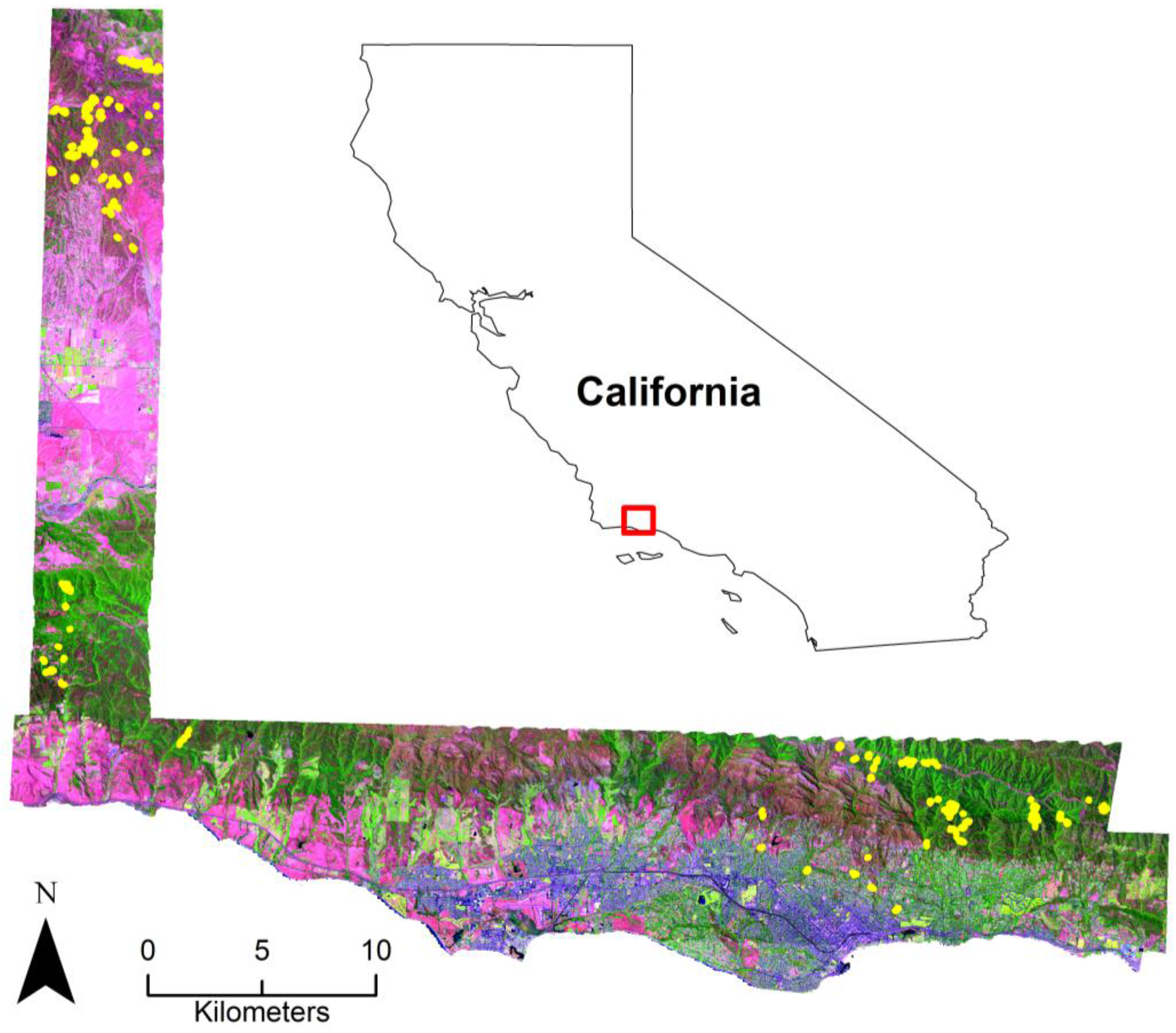
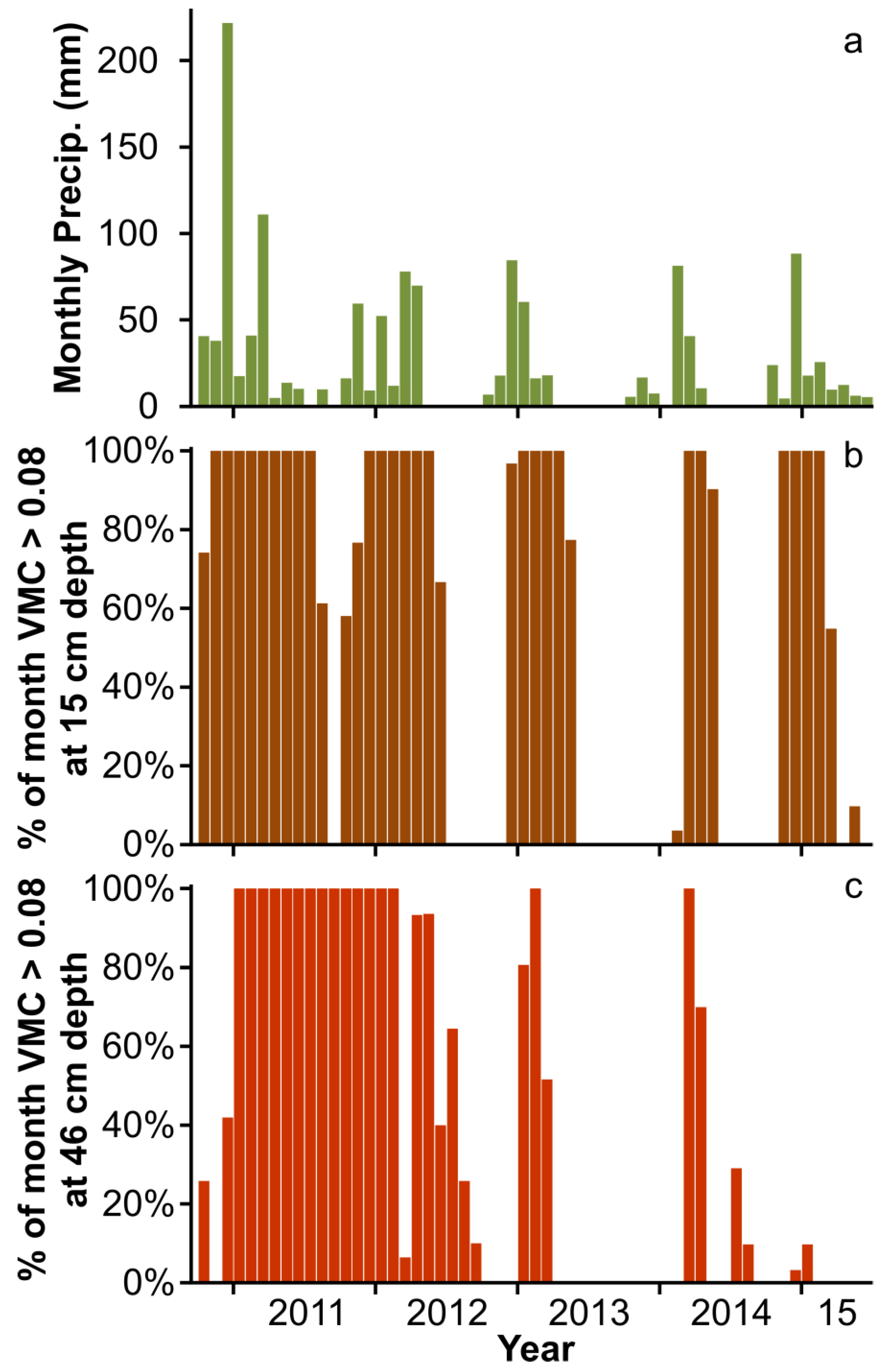
2.1. Study Area
2.2. Image Data
2.3. Ground Reference Data
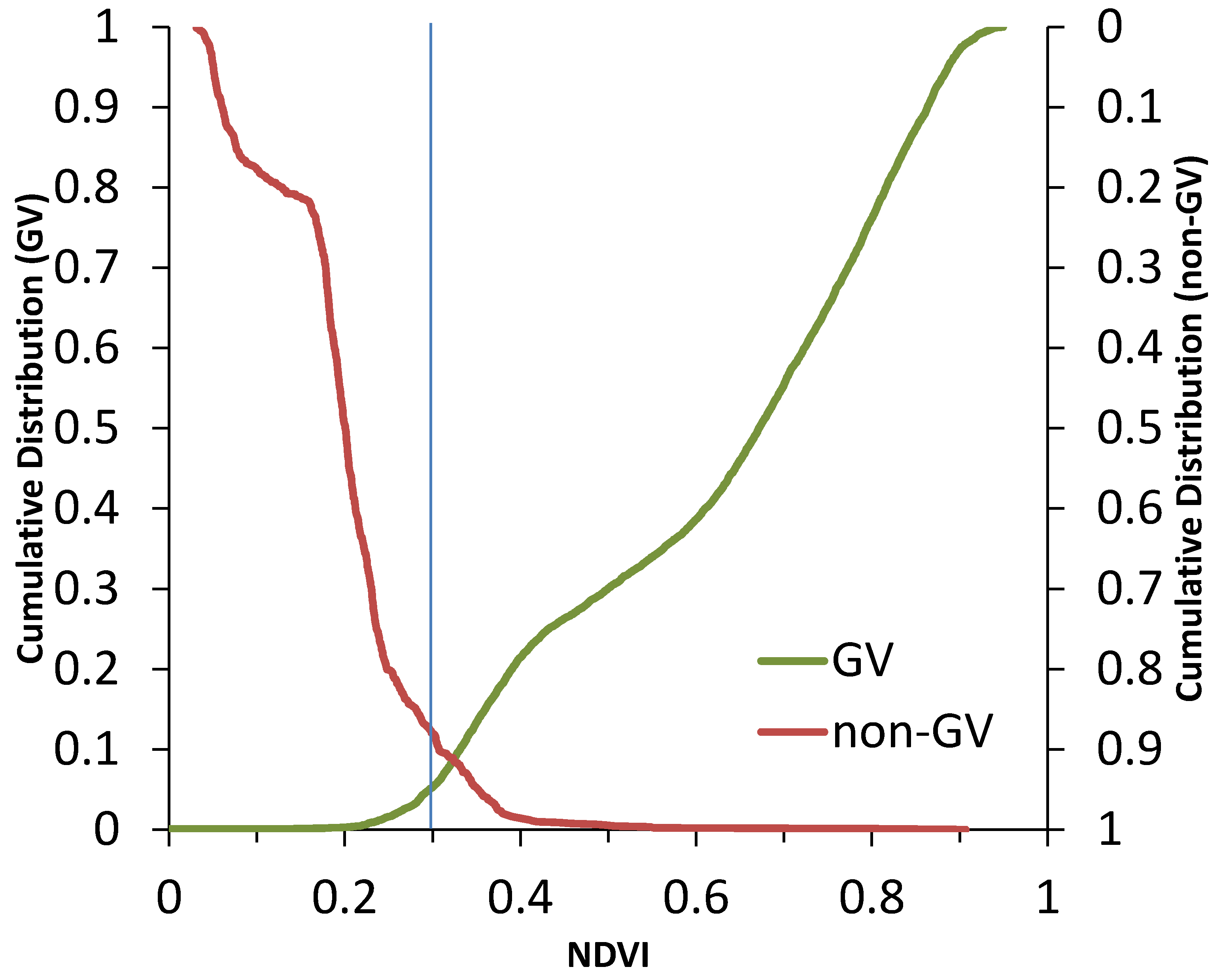
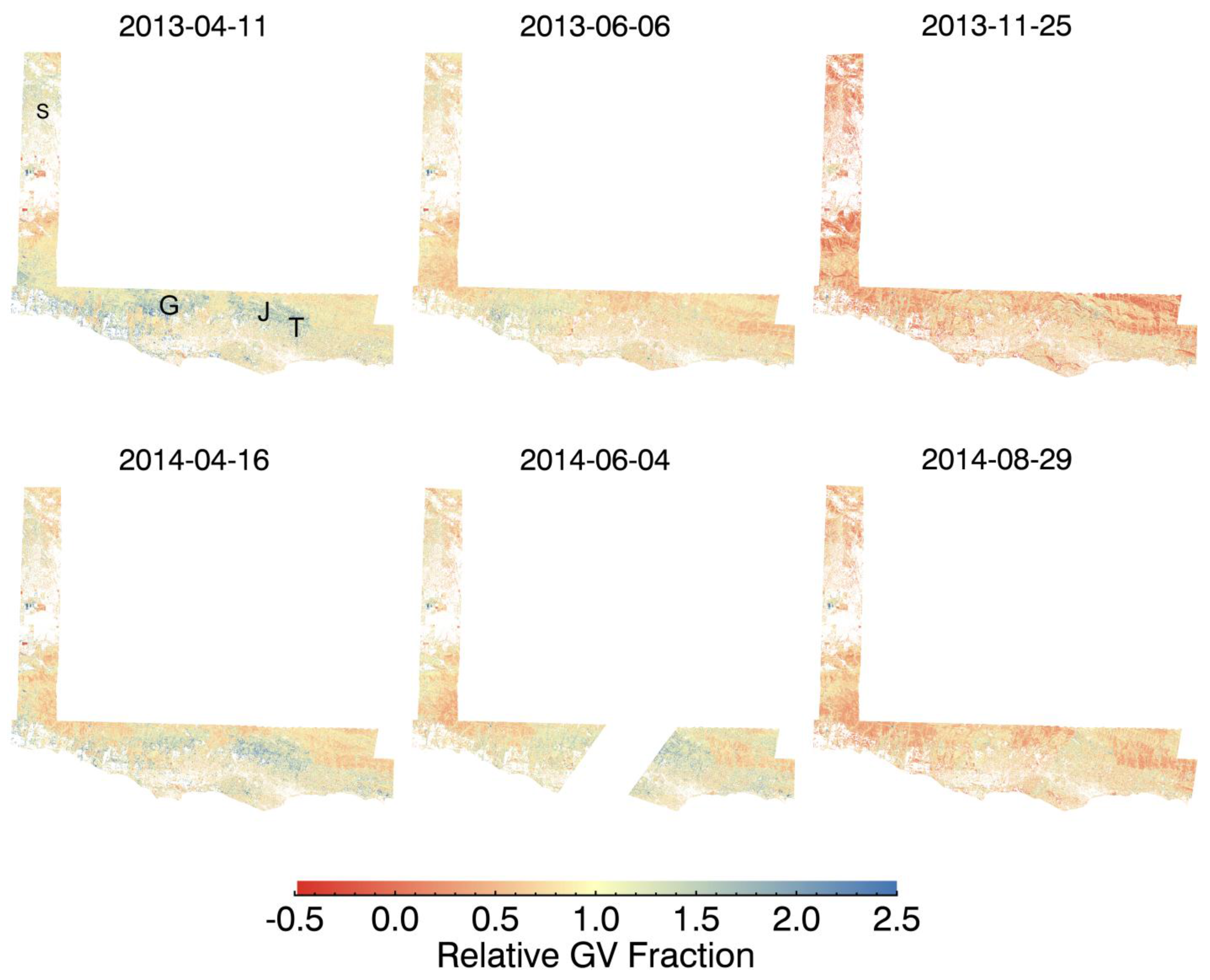
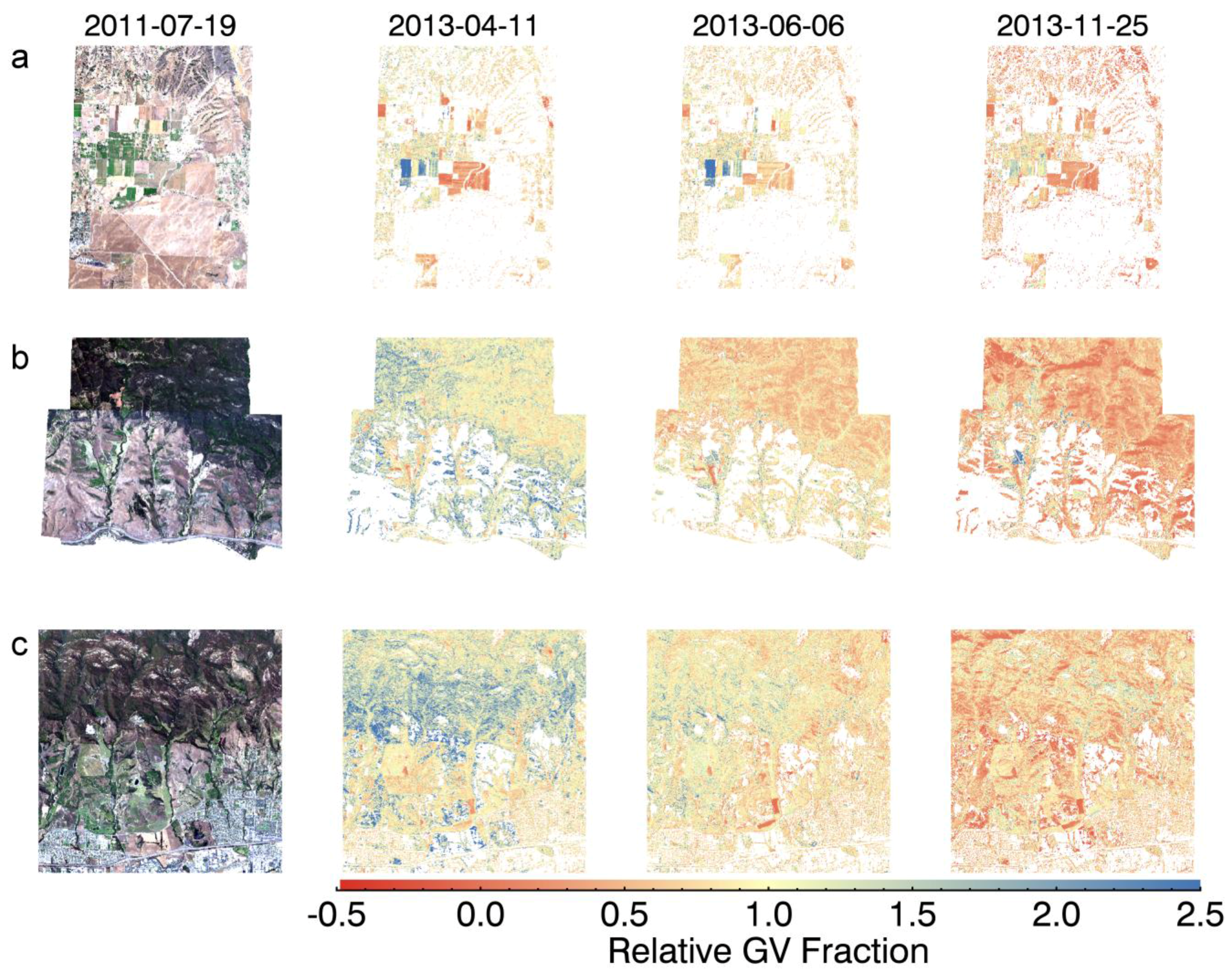
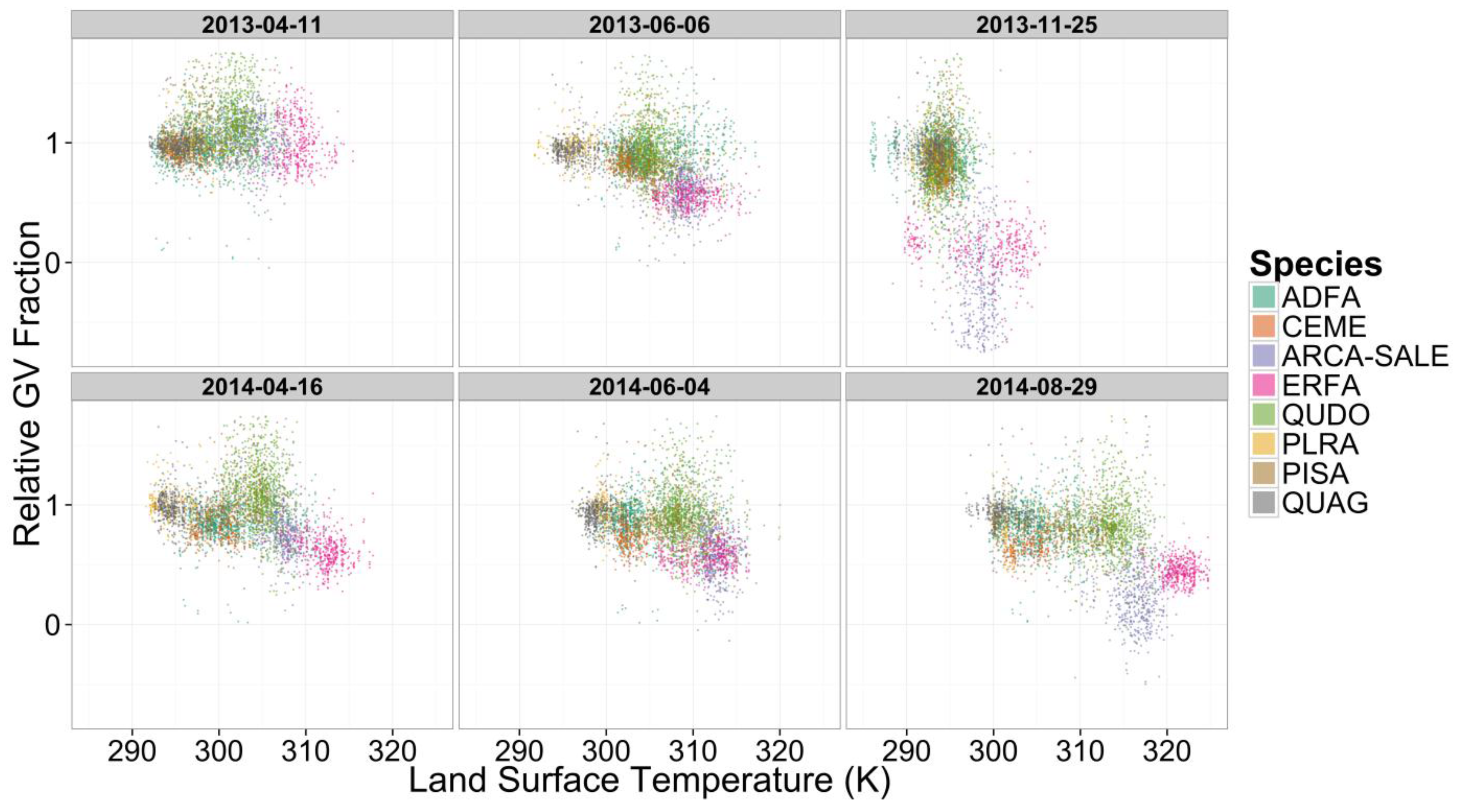
2.4. Analysis

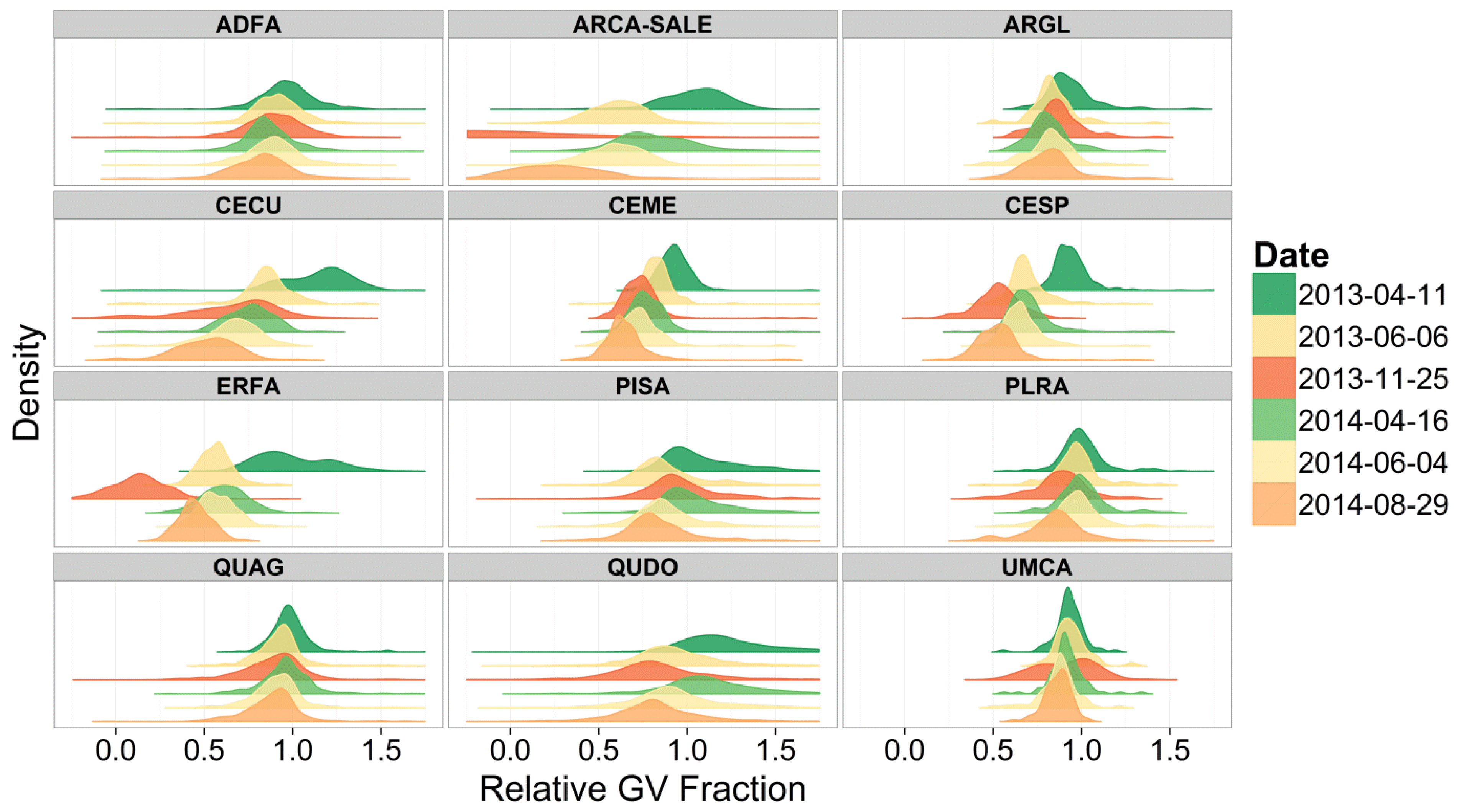
| Species/Vegetation Type | Code | Functional Type | N Pixels |
|---|---|---|---|
| Adenostoma fasciculatum | ADFA | evergreen chaparral | 2727 |
| Artemisia californica-Salvia leucophylla | ARCA-SALE | coastal sage scrub | 1548 |
| Arctostaphylos glauca/glandulosa | ARGL | evergreen chaparral | 342 |
| Ceanothus cuneatus | CECU | evergreen chaparral | 318 |
| Ceanothus megacarpus | CEME | evergreen chaparral | 720 |
| Ceanothus spinosus | CESP | evergreen chaparral | 957 |
| Eriogonum fasciculatum | ERFA | coastal sage scrub | 1212 |
| Pinus sabiniana | PISA | evergreen tree | 1203 |
| Platanus racemosa | PLRA | deciduous tree | 720 |
| Quercus agrifolia | QUAG | evergreen tree | 1536 |
| Quercus douglasii | QUDO | deciduous tree | 2769 |
| Umbellularia californica | UMCA | evergreen tree | 249 |


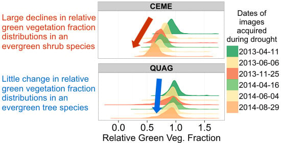
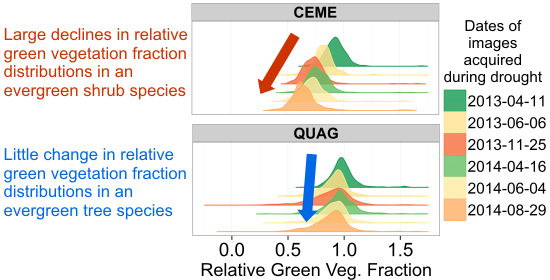
3. Results and Discussion


4. Conclusions
Acknowledgements
Author Contributions
Conflicts of Interest
References
- Griffin, D.; Anchukaitis, K.J. How unusual is the 2012–2014 California drought? Geophys. Res. Lett. 2014, 41, 9017–9023. [Google Scholar] [CrossRef]
- Diffenbaugh, N.S.; Swain, D.L.; Touma, D. Anthropogenic warming has increased drought risk in California. Proc. Natl. Acad. Sci. USA 2015, 112, 3931–3936. [Google Scholar] [CrossRef] [PubMed]
- Anderegg, W.R.; Flint, A.; Huang, C.-Y.; Flint, L.; Berry, J.A.; Davis, F.W.; Sperry, J.S.; Field, C.B. Tree mortality predicted from drought-induced vascular damage. Nat. Geosci. 2015. [Google Scholar] [CrossRef]
- Bréda, N.; Huc, R.; Granier, A.; Dreyer, E. Temperate forest trees and stands under severe drought: A review of ecophysiological responses, adaptation processes and long-term consequences. Ann. For. Sci. 2006, 63, 625–644. [Google Scholar] [CrossRef]
- McDowell, N.G.; Pockman, W.T.; Allen, C.D.; Breshears, D.D.; Cobb, N.; Kolb, T.; Plaut, J.; Sperry, J.; West, A.; Williams, D.G. Mechanisms of plant survival and mortality during drought: Why do some plants survive while others succumb to drought? New Phytol. 2008, 178, 719–739. [Google Scholar] [CrossRef] [PubMed]
- McDowell, N.G.; Fisher, R.A.; Xu, C.; Domec, J.; Hölttä, T.; Mackay, D.S.; Sperry, J.S.; Boutz, A.; Dickman, L.; Gehres, N. Evaluating theories of drought-induced vegetation mortality using a multimodel–experiment framework. New Phytol. 2013, 200, 304–321. [Google Scholar] [CrossRef] [PubMed]
- Davis, S.D.; Ewers, F.W.; Sperry, J.S.; Portwood, K.A.; Crocker, M.C.; Adams, G.C. Shoot dieback during prolonged drought in ceanothus (rhamnaceae) chaparral of California: A possible case of hydraulic failure. AmJ. Bot. 2002, 89, 820–828. [Google Scholar] [CrossRef] [PubMed]
- Choat, B.; Jansen, S.; Brodribb, T.J.; Cochard, H.; Delzon, S.; Bhaskar, R.; Bucci, S.J.; Feild, T.S.; Gleason, S.M.; Hacke, U.G. Global convergence in the vulnerability of forests to drought. Nature 2012, 491, 752–755. [Google Scholar] [CrossRef] [PubMed]
- Maherali, H.; Pockman, W.T.; Jackson, R.B. Adaptive variation in the vulnerability of woody plants to xylem cavitation. Ecology 2004, 85, 2184–2199. [Google Scholar] [CrossRef]
- Miller, P.C.; Poole, D.K. Patterns of water use by shrubs in southern California. For. Sci. 1979, 25, 84–98. [Google Scholar]
- Royce, E.B.; Barbour, M.G. Mediterranean climate effects. I. Conifer water use across a Sierra Nevada ecotone. Am. J. Bot. 2001, 88, 911–918. [Google Scholar] [CrossRef] [PubMed]
- Canadell, J.; Jackson, R.; Ehleringer, J.; Mooney, H.; Sala, O.; Schulze, E.-D. Maximum rooting depth of vegetation types at the global scale. Oecologia 1996, 108, 583–595. [Google Scholar] [CrossRef]
- Jacobsen, A.L.; Pratt, R.B.; Davis, S.D.; Ewers, F.W. Comparative community physiology: Nonconvergence in water relations among three semi-arid shrub communities. New Phytol. 2008, 180, 100–113. [Google Scholar] [CrossRef] [PubMed]
- Jacobsen, A.L.; Pratt, R.B.; Davis, S.D.; Tobin, M.F. Geographic and seasonal variation in chaparral vulnerability to cavitation. Madroño 2014, 61, 317–327. [Google Scholar] [CrossRef]
- Asner, G.P.; Jones, M.O.; Martin, R.E.; Knapp, D.E.; Hughes, R.F. Remote sensing of native and invasive species in Hawaiian forests. Remote Sens. Environ. 2008, 112, 1912–1926. [Google Scholar] [CrossRef]
- Ustin, S.L.; Gitelson, A.A.; Jacquemoud, S.; Schaepman, M.; Asner, G.P.; Gamon, J.A.; Zarco-Tejada, P. Retrieval of foliar information about plant pigment systems from high resolution spectroscopy. Remote Sens. Environ. 2009, 113, S67–S77. [Google Scholar] [CrossRef] [Green Version]
- Serbin, S.P.; Singh, A.; McNeil, B.E.; Kingdon, C.C.; Townsend, P.A. Spectroscopic determination of leaf morphological and biochemical traits for northern temperate and boreal tree species. Ecol. Appl. 2014, 24, 1651–1669. [Google Scholar] [CrossRef]
- Serbin, S.P.; Singh, A.; Desai, A.R.; Dubois, S.G.; Jablonski, A.D.; Kingdon, C.C.; Kruger, E.L.; Townsend, P.A. Remotely estimating photosynthetic capacity, and its response to temperature, in vegetation canopies using imaging spectroscopy. Remote Sens. Environ. 2015, 167, 78–87. [Google Scholar] [CrossRef]
- Dennison, P.E.; Roberts, D.A. The effects of vegetation phenology on endmember selection and species mapping in southern California chaparral. Remote Sens. Environ. 2003, 87, 295–309. [Google Scholar] [CrossRef]
- Dudley, K.L.; Dennison, P.E.; Roth, K.L.; Roberts, D.A.; Coates, A.R. A multi-temporal spectral library approach for mapping vegetation species across spatial and temporal phenological gradients. Remote Sens. Environ. 2015, 167, 121–134. [Google Scholar] [CrossRef]
- Roth, K.L.; Roberts, D.A.; Dennison, P.E.; Alonzo, M.; Peterson, S.H.; Beland, M. Differentiating plant species within and across diverse ecosystems with imaging spectroscopy. Remote Sens. Environ. 2015, 167, 135–151. [Google Scholar] [CrossRef]
- Féret, J.-B.; Asner, G.P. Tree species discrimination in tropical forests using airborne imaging spectroscopy. IEEE Trans. Geosci. Remote Sens. 2013, 51, 73–84. [Google Scholar] [CrossRef]
- Clark, M.L.; Roberts, D.A.; Clark, D.B. Hyperspectral discrimination of tropical rain forest tree species at leaf to crown scales. Remote Sens. Environ. 2005, 96, 375–398. [Google Scholar] [CrossRef]
- Baldeck, C.; Colgan, M.; Féret, J.-B.; Levick, S.R.; Martin, R.; Asner, G. Landscape-scale variation in plant community composition of an African savanna from airborne species mapping. Ecol. Appl. 2014, 24, 84–93. [Google Scholar] [CrossRef] [PubMed]
- Asner, G.P.; Nepstad, D.; Cardinot, G.; Ray, D. Drought stress and carbon uptake in an Amazon forest measured with spaceborne imaging spectroscopy. Proc. Natl. Acad. Sci. USA 2004, 101, 6039–6044. [Google Scholar] [CrossRef] [PubMed]
- Dennison, P.E.; Roberts, D.A.; Thorgusen, S.R.; Regelbrugge, J.C.; Weise, D.; Lee, C. Modeling seasonal changes in live fuel moisture and equivalent water thickness using a cumulative water balance index. Remote Sens. Environ. 2003, 88, 442–452. [Google Scholar] [CrossRef]
- Otkin, J.A.; Anderson, M.C.; Hain, C.; Mladenova, I.E.; Basara, J.B.; Svoboda, M. Examining rapid onset drought development using the thermal infrared–based evaporative stress index. J. Hydrometeorol. 2013, 14, 1057–1074. [Google Scholar] [CrossRef]
- Wan, Z.; Wang, P.; Li, X. Using MODIS land surface temperature and normalized difference vegetation index products for monitoring drought in the southern great plains, USA. Int. J. Remote Sens. 2004, 25, 61–72. [Google Scholar] [CrossRef]
- Anderson, M.C.; Allen, R.G.; Morse, A.; Kustas, W.P. Use of Landsat thermal imagery in monitoring evapotranspiration and managing water resources. Remote Sens. Environ. 2012, 122, 50–65. [Google Scholar] [CrossRef]
- Roberts, D.A.; Dennison, P.E.; Roth, K.L.; Dudley, K.; Hulley, G. Relationships between dominant plant species, fractional cover and land surface temperature in a Mediterranean ecosystem. Remote Sens. Environ. 2015, 167, 152–167. [Google Scholar] [CrossRef]
- Lee, C.M.; Cable, M.L.; Hook, S.J.; Green, R.O.; Ustin, S.L.; Mandl, D.J.; Middleton, E.M. An introduction to the NASA Hyperspectral Infrared Imager (HyspIRI) mission and preparatory activities. Remote Sens. Environ. 2015, 167, 6–19. [Google Scholar] [CrossRef]
- Hochberg, E.J.; Roberts, D.A.; Dennison, P.E.; Hulley, G.C. Special issue on the Hyperspectral Infrared Imager (HyspIRI): Emerging science in terrestrial and aquatic ecology, radiation balance and hazards. Remote Sens. Environ. 2015, 167, 1–5. [Google Scholar] [CrossRef]
- Green, R.O.; Eastwood, M.L.; Sarture, C.M.; Chrien, T.G.; Aronsson, M.; Chippendale, B.J.; Faust, J.A.; Pavri, B.E.; Chovit, C.J.; Solis, M. Imaging spectroscopy and the Airborne Visible/Infrared Imaging Spectrometer (AVIRIS). Remote Sens. Environ. 1998, 65, 227–248. [Google Scholar] [CrossRef]
- Hook, S.J.; Myers, J.J.; Thome, K.J.; Fitzgerald, M.; Kahle, A.B. The MODIS/ASTER airborne simulator (MASTER)—A new instrument for earth science studies. Remote Sens. Environ. 2001, 76, 93–102. [Google Scholar] [CrossRef]
- Roberts, D.A.; Bradley, E.; Roth, K.; Eckmann, T.; Still, C. Linking physical geography education and research through the development of an environmental sensing network and project-based learning. J. Geosci. Educ. 2010, 58, 262–274. [Google Scholar] [CrossRef]
- Thompson, D.R.; Gao, B.-C.; Green, R.O.; Roberts, D.A.; Dennison, P.E.; Lundeen, S.R. Atmospheric correction for global mapping spectroscopy: ATREM advances for the HyspIRI preparatory campaign. Remote Sens. Environ. 2015, 167, 64–77. [Google Scholar] [CrossRef]
- Hulley, G. HyspIRI level-2 thermal infrared (TIR) land surface temperature and emissivity algorithm theoretical basis document; Jet Propulsion Laboratory, National Aeronautics and Space Administration: Pasadena, CA, USA, 2011. [Google Scholar]
- Hulley, G.C.; Hughes, C.G.; Hook, S.J. Quantifying uncertainties in land surface temperature and emissivity retrievals from ASTER and MODIS thermal infrared data. J. Geophys. Res. Atmos. 2012. [Google Scholar] [CrossRef]
- Grigsby, S.P.; Hulley, G.C.; Roberts, D.A.; Scheele, C.; Ustin, S.L.; Alsina, M.M. Improved surface temperature estimates with MASTER/AVIRIS sensor fusion. Remote Sens. Environ. 2015, 167, 53–63. [Google Scholar] [CrossRef]
- Meentemeyer, R.K.; Moody, A. Rapid sampling of plant species composition for assessing vegetation patterns in rugged terrain. Landsc. Ecol. 2000, 15, 697–711. [Google Scholar] [CrossRef]
- Roth, K.L.; Dennison, P.E.; Roberts, D.A. Comparing endmember selection techniques for accurate mapping of plant species and land cover using imaging spectrometer data. Remote Sens. Environ. 2012, 127, 139–152. [Google Scholar] [CrossRef]
- Adams, J.B.; Smith, M.O.; Gillespie, A.R. Imaging spectroscopy: Interpretation based on spectral mixture analysis. Remote Geochem. Anal.: Elemental Mineral. Compos. 1993, 7, 145–166. [Google Scholar]
- Roberts, D.A.; Smith, M.O.; Adams, J.B. Green vegetation, nonphotosynthetic vegetation, and soils in AVIRIS data. Remote Sens. Environ. 1993, 44, 255–269. [Google Scholar] [CrossRef]
- Okin, G.S. Relative spectral mixture analysis—A multitemporal index of total vegetation cover. Remote Sens. Environ. 2007, 106, 467–479. [Google Scholar] [CrossRef]
- Somers, B.; Asner, G.P.; Tits, L.; Coppin, P. Endmember variability in spectral mixture analysis: A review. Remote Sens. Environ. 2011, 115, 1603–1616. [Google Scholar] [CrossRef]
- Meyer, T.; Okin, G. Evaluation of spectral unmixing techniques using MODIS in a structurally complex savanna environment for retrieval of green vegetation, nonphotosynthetic vegetation, and soil fractional cover. Remote Sens. Environ. 2015, 161, 122–130. [Google Scholar] [CrossRef]
- Roberts, D.A.; Gardner, M.; Church, R.; Ustin, S.; Scheer, G.; Green, R. Mapping chaparral in the Santa Monica Mountains using multiple endmember spectral mixture models. Remote Sens. Environ. 1998, 65, 267–279. [Google Scholar] [CrossRef]
- Hellmers, J.; Horton, J.S.; Juhren, G.; O'Keefe, J.O. Root systems of some chaparral plants in southern california. Ecol. 1955, 36, 667–678. [Google Scholar] [CrossRef]
- Gower, S.T.; Kucharik, C.J.; Norman, J.M. Direct and indirect estimation of leaf area index, f(apar), and net primary production of terrestrial ecosystems. Remote Sens. Environ. 1999, 70, 29–51. [Google Scholar] [CrossRef]
- Scherrer, D.; Bader, M.K.-F.; Körner, C. Drought-sensitivity ranking of deciduous tree species based on thermal imaging of forest canopies. Agric. For. Meteorol. 2011, 151, 1632–1640. [Google Scholar] [CrossRef]
- Guardiola-Claramonte, M.; Troch, P.A.; Breshears, D.D.; Huxman, T.E.; Switanek, M.B.; Durcik, M.; Cobb, N.S. Decreased streamflow in semi-arid basins following drought-induced tree die-off: A counter-intuitive and indirect climate impact on hydrology. J. Hydrol. 2011, 406, 225–233. [Google Scholar] [CrossRef]
- Royer, P.D.; Cobb, N.S.; Clifford, M.J.; Huang, C.Y.; Breshears, D.D.; Adams, H.D.; Villegas, J.C. Extreme climatic event-triggered overstorey vegetation loss increases understorey solar input regionally: Primary and secondary ecological implications. J. Ecol. 2011, 99, 714–723. [Google Scholar] [CrossRef]
- Mueller, R.C.; Scudder, C.M.; Porter, M.E.; Talbot Trotter, R.; Gehring, C.A.; Whitham, T.G. Differential tree mortality in response to severe drought: Evidence for long-term vegetation shifts. J. Ecol. 2005, 93, 1085–1093. [Google Scholar] [CrossRef]
© 2015 by the authors; licensee MDPI, Basel, Switzerland. This article is an open access article distributed under the terms and conditions of the Creative Commons Attribution license (http://creativecommons.org/licenses/by/4.0/).
Share and Cite
Coates, A.R.; Dennison, P.E.; Roberts, D.A.; Roth, K.L. Monitoring the Impacts of Severe Drought on Southern California Chaparral Species using Hyperspectral and Thermal Infrared Imagery. Remote Sens. 2015, 7, 14276-14291. https://doi.org/10.3390/rs71114276
Coates AR, Dennison PE, Roberts DA, Roth KL. Monitoring the Impacts of Severe Drought on Southern California Chaparral Species using Hyperspectral and Thermal Infrared Imagery. Remote Sensing. 2015; 7(11):14276-14291. https://doi.org/10.3390/rs71114276
Chicago/Turabian StyleCoates, Austin R., Philip E. Dennison, Dar A. Roberts, and Keely L. Roth. 2015. "Monitoring the Impacts of Severe Drought on Southern California Chaparral Species using Hyperspectral and Thermal Infrared Imagery" Remote Sensing 7, no. 11: 14276-14291. https://doi.org/10.3390/rs71114276