On Uncertainties of the Priestley-Taylor/LST-Fc Feature Space Method to Estimate Evapotranspiration: Case Study in an Arid/Semiarid Region in Northwest China

Abstract

Accurate evapotranspiration (ET) estimation is very crucial for water resource management, particularly for the arid and semi-arid region. The remote sensing-based Priestley-Taylor method (RS-PT method) can estimate ET at regional scale, using the feature space of remotely sensed land surface temperature (LST) and vegetation index (VI). This study evaluates the RS-PT feature space method over an arid and semi-arid region in northwest China using satellite data from the moderate-resolution space-borne sensor Advanced Along-Track Scanning Radiometer (AATSR), the observations from the high-resolution airborne sensor Wide-angle Infrared Dual-mode line/area Array Scanner (WiDAS) and ground measurements of heat fluxes collected in summer 2008. The results show that the mean difference for latent heat flux (LE) estimates resulting from different domain sizes is 69.5 W/m². When using high-resolution images from airborne measurements, the dry boundary is strongly affected by the pixels of impervious surfaces, which lead to a mean difference of 15.36 W/m² for LE estimates. In addition, the physically based Surface Energy Balance Index (SEBI) model is used to analyze the accuracy of dry/wet boundaries in the RS-PT method. Compared with the SEBI-estimated relative evaporative fraction (Λ_r), the RS-PT method underestimated Λ_r by ~0.11. For the RS-PT method, the uncertainty in the determination of the dry/wet boundaries has a significant impact on the accuracy of the ET estimate, not only depending on the size of the area to build the feature space, but also on the land covers.

1. Introduction

Evapotranspiration (ET) is of great importance in modeling the water and energy interactions between land and atmosphere, and is a primary process in the energy and water exchange between hydrosphere, atmosphere and biosphere in terrestrial ecosystems. A precise estimation of regional ET is considered essential for many applications, such as global environmental change, regional ecosystem, water resource management and sustainable development of agriculture.

Traditional techniques provide point measurements, which usually are not representative of large regions due to the heterogeneity of the land surfaces and the dynamic nature of heat transfer. The development of remote sensing techniques provides a unique opportunity to estimate regional ET [1]. Many methods using remotely sensed data to acquire the spatially continuous ET have been proposed in the last few decades, including surface energy balance based models, empirical statistical methods, the traditional ET estimation approaches based on Penman-Monteith (PM) equation, methods based on land surface model and data assimilation techniques [2,3,4], all of which have been shown to provide acceptable results over certain range of land cover types and conditions [5,6].

Land surface ET is affected by numerous factors, including soil properties, weather condition, plant biophysics, and surface available energy, which have all been embedded in many physical based algorithms. However, difficulties in acquiring spatially representative ancillary measurements (e.g., near surface meteorological data, soil properties, and plant biophysical information) and in parameterization of various surface resistances, also have hindered the application of methods based on physical parameterization for ET estimation. As for the methods based on land surface model and data assimilation techniques, they need a lot of data and parameterizations as inputs and are relatively more computationally demanding than the remote sensing ET models. The empirical and semi-empirical statistical models, due to the lack of the physical foundation, need calibration to be applicable to local climate and ecosystems. Alternatively, methods built upon the triangle space between the land surface temperature (LST) and vegetation index (VI) e.g., Normalized Difference Vegetation Index (NDVI) and vegetation fractional cover (Fc) (referred to as the LST-Fc method) have been developed and widely used to estimate ET, evaporative fraction (EF) and soil moisture due to their simplicity and minimal request for inputs [7,8,9,10,11]. For instance, Jiang and Islam (1999) applied the triangle feature space method from the remotely sensed LST and NDVI to modify the coefficient of the Priestley-Taylor equation for actual ET estimates, which is called the RS-PT method. Such a method gives a clear physical meaning to the coefficient of the Priestley-Taylor equation and has been validated by several studies [12,13,14,15,16].

However, there are some uncertainties and limitations associated with the LST-Fc space method. Long et al. [17] assessed domain size dependencies of the LST-Fc feature space method using Landsat Thematic Mapper/Enhanced Thematic (TM/ETM) at the Soil Moisture-Atmosphere Coupling Experiment site in 2002. They indicated that the dry edge of the triangle method tends to move upward and the wet edge tends to move in the opposite direction when the domain size is increased, which could cause the a large uncertainties in EF estimates in terms of a mean absolute percentage difference (MAPD) up to 50%. Tian et al. [18] also quantitatively investigated variation of limiting edges due to the spatial domain size using ten Moderate Resolution Imaging Spectroradiometer (MODIS) observations in the Heihe River basin during growing season in 2009. Results showed that the extreme high surface temperature tends to increase and the extreme low surface temperature tends to decrease with the increase of domain size. Variation of intercept and slope of the dry edge would lead to the deviation in ET estimates with the maximum of 66 W/m². Deviated from the previous studies, this study focuses primarily on offer a comprehensive view of the uncertainty in RS-PT method from a perspective of model physics and practical application through a study over arid/semiarid region in northwest China, including the preconditions of this methods and the influence of domain size as well as high-resolution scale effects. In addition, this study examines the accuracy of dry/wet boundaries from LST-Fc feature space by using a theoretical wet/dry edges derived from the physically based Surface Energy Balance Index (SEBI) model. Section 2 introduces fundamentals of RS-PT method and the theoretical dry/wet boundaries to assess dry/wet boundaries from LST-Fc feature space, followed by a description of study area and data collection in Section 3. Section 4 provides a systematic analysis of the uncertainties of RS-PT in application using moderate and high resolutions images, respectively, and a comparison between statistical and theoretical dry/wet boundaries. Conclusions and summaries are given in Section 5.

2. Methodology

2.1. Brief Overview of RS-PT Methods

2.1.1. The LST-Fc Feature Space

Although NDVI is commonly used as the VI in the RS-PT method, Fc is considered to be more appropriate than NDVI in the LST-VI diagram [15]. Therefore, we use Fc to construct the LST-VI triangle feature space. As shown in the LST-Fc diagram (Figure 1), point A represents the dry bare soil pixels with maximum LST and minimum Fc, point B represents well-watered soil at the potential ET with minimum LST. Point C represents well-watered vegetation pixels at potential ET and with minimum LST and maximum Fc. In Figure 1, the line AC is called the “dry edge”, along which Fc increases with decreasing LST under extreme dry surface conditions. The line BC is called the “wet edge”, along which the LST varies with the increase of Fc with potential ET (defined as the evaporation rate that would occur from a saturated surface with constant energy supply and constant atmospheric conditions). The wet and dry edges are derived statistically using linear regressions between the LST and Fc in the feature space diagram, for well-watered soil-vegetation canopy and completely dry soil conditions, respectively.

Figure 1. The concept of the LST-Fc triangular feature space.

Figure 1. The concept of the LST-Fc triangular feature space.

In an ideal diagram, there is a point above the point C, which represents closed canopy pixels under water stress. The diagram would thus be a typical trapezoidal feature space [7]. However, in most practical applications using data from various remote sensors, this point is poorly defined or the position is very close to point C, so that a typical triangle shape in LST-Fc feather space is more often observed [8].

2.1.2. The RS-PT Method

The Priestley-Taylor equation, which has a clear physical meaning, has been widely used to calculate potential ET, provided advection can be neglected [19]:

$$LE=\mathrm{\alpha }[(R_{\mathrm{n}}-G)\frac{\mathrm{\Delta }}{\mathrm{\Delta }+\gamma }]$$

(1)

where LE (W/m²) is latent heat flux, α is the Priestley-Taylor (P-T) parameter, R_n and G (W/m²) are the net radiation flux and soil heat flux, respectively; Δ (Pa/K) is the slope of saturated vapor pressure with air temperature, and γ (Pa/K) is the psychometric constant. For well-watered soil-vegetation canopies, α is set as 1.26 [19]. Jiang and Islam proposed a modified version of the PT equation, which is to parameterize the P-T coefficient α based on the remotely sensed LST-VI feature space [12]. This method is referred to as the “remote sensing based Priestley-Taylor method” (RS-PT for short), and the symbol ϕ is used for the parameterized P-T coefficient, replacing the original coefficient α.

In the RS-PT model, the dry/wet boundaries in Figure 1 are straight lines and can be determined by a regression method applied to the scatter plot of LST and Fc. In this paper, the dry/wet boundaries are determined by an approach based on the scheme proposed by Tang et al., [15]. The value of ϕ for point A in Figure 1, corresponding to the driest soil with the lowest Fc, is set to 0. The value of ϕ for point B at the position of minimal Fc and minimal LST is set to 1.26. The value of ϕ along the wet edge is taken the same as that of point B, referred to ϕ_max (= 1.26). The actual pixel-wise coefficient ϕ is derived using a two-steps interpolation scheme in the LST-Fc triangular space, as given below.

Firstly, the value of ϕ on the dry edge, referred as ϕ_min,Fc, is linearly interpolated between 0 and 1.26 and changing with Fc,

$${\varphi }_{\text{min},Fc}=1.26F_c$$

(2)

Secondly, the ϕ values under the same F_c are linearly interpolated between ϕ_min,Fc and ϕ_max, increasing with the decrease of LST [10,12],

$$\varphi =\frac{T_{\text{max},Fc}-T_i}{T_{\text{max},Fc}-T_{\text{min},Fc}}({\varphi }_{\text{max}}-{\varphi }_{\text{min},Fc})+{\varphi }_{\text{min},Fc}$$

(3)

where T_max,Fc and T_min,Fc are LST values on the dry and wet edges, respectively, for any given F_C. The T_i is the LST of pixel i (K).

The decrease of LST along the dry edge is due to the increase of the transpiration from vegetation with increasing Fc. For any given Fc, the ϕ increases linearly with LST, bounded by the ϕ values on the respective dry and wet edges (Equation (3)). In the LST-Fc triangle space, for a given F_C, the relative size of LST is the indication of the soil moisture and the LST variation among different pixels is caused by the variation of soil moisture. Therefore, the LST-Fc triangle space implies that the LST is only affected by the variation of soil moisture and Fc, rather than by other factors, such as different atmospheric conditions or the topographical heterogeneity of the region [20,21,22].

From the above analysis, we can summarize the assumption and hypothesis in the RS-PT method as follows. (1) The dry/wet boundaries determined by the statistical method in the LST-Fc feature space are very close to the theoretical values; (2) For a given Fc, the evaporative fraction (EF) is a linear function of soil moisture availability; (3) The area of interest is under homogenous atmospheric forcing and with relatively small variations in terrain elevation.

2.2. Theoretical Dry/Wet Boundaries

In this study, SEBI algorithm proposed by Menenti and Choudhury [23] is used to obtain the theoretical-based dry/wet boundaries in the LST-Fc feature space. A brief description of SEBI is given below.

The relative evaporation fraction Λ_r, defined as the ratio of actual ET (λE) to potential ET (λE_p), is expressed as:

$${\mathrm{\Lambda }}_r=\lambda E/\lambda E_P=1-SEBI$$

(4)

where SEBI, according to Menenti and Choudhury (1993), is an index of standardized difference of temperature difference between the land surface and the air scaled by its dry and wet conditions and given below:

$$SEBI=\frac{\frac{(T_s-T_a)}{{\mathrm{r}}_{\mathrm{a}}}-\frac{(T_{s,w}-T_a)}{{\mathrm{r}}_{\text{a,w}}}}{\frac{(T_{s,d}-T_a)}{{\mathrm{r}}_{\text{a,d}}}-\frac{(T_{s,w}-T_a)}{{\mathrm{r}}_{\text{a,w}}}}$$

(5)

where T_s (K) is the land surface temperature, T_a (K) is the air temperature at reference height, T_s,w is the temperature at the wet-limit, T_s,d is the temperature at the dry-limit.

The (T_s,d – T_a) in Equation (5) is the surface-air temperature difference corresponding to the extreme dry condition:

$$T_{s,d}-T_a=(r_{a,\mathrm{d}})\frac{R_n-G}{\rho C_p}$$

(6)

where ρ (kg∙m⁻³) is the air density; C_p (= 1005 J∙kg⁻¹∙K⁻¹) is the specific heat of air at constant pressure.

The (T_s,w − T_a) in Equation (5) is the surface-air temperature difference for wet condition:

$$T_{s,w}-T_a=\frac{(r_{a,w})\frac{R_n-G}{\rho C_p}-\frac{1}{\gamma }(e_{sat}-e)}{1+\frac{\mathrm{\Delta }}{\gamma }}$$

(7)

where Δ (Pa/K) is the slope of e with air temperature and γ (Pa/K) is the psychometric constant, as before; e (Pa) is actual vapor pressure near surface; e_sat (Pa) is the saturated vapor pressure at mean air temperature. The r_a (s∙m⁻¹) in Equation (5) is the aerodynamic resistance and expressed as:

$$r_a=\frac{1}{k{u}_{*}}[\text{ln}(\frac{z-d_0}{z_{0h}})-{\psi }_h(\frac{\mathrm{z}-d_0}{L})+{\psi }_h(\frac{{\mathrm{z}}_{0h}}{L})]$$

(8)

where k is the von Karman constant (k = 0.4), z (m) is the reference height, z_oh (m) is the roughness length for heat transfer, d₀ (m) is the zero plane displacement height, $u_{*}$ (m∙s⁻¹) is the friction velocity, Ψ_h is the stability correction function for turbulent heat flux.

The aerodynamic resistance for the theoretical boundaries, i.e., r_a,d for zero evaporation (dry extreme) and r_a,w for potential evaporation (wet extreme) are respectively defined as

$$r_{a,d}=\frac{1}{k{u}_{*}}[\text{ln}(\frac{z-d_0}{z_{0h}})-{\psi }_h(\frac{\mathrm{z}-d_0}{L_d})+{\psi }_h(\frac{Z_{0h}}{L_d})]$$

(9)

$$r_{a,w}=\frac{1}{k{u}_{*}}[\text{ln}(\frac{z-d_0}{z_{0h}})-{\psi }_h(\frac{\mathrm{z}-d_0}{L_w})+{\psi }_h(\frac{Z_{0h}}{L_w})]$$

(10)

The L (m) in Equation (8) is the Monin-Obukhov length and defined as,

$$L=-\frac{\rho C_p{u_{*}}^3{\mathrm{\theta }}_v}{kgH}$$

(11)

where g (m∙s⁻²) is the acceleration due to gravity, θ_v (K) is the potential virtual temperature near the surface.

In Equations (9) and (10), the Monin-Obukhov length for the two extreme limits are expressed, respectively, as,

$$L_{\mathrm{w}}=-\frac{{\rho }_a{u_{*}}^3}{kg(\frac{H_w}{c_p{T}_a}+0.608\frac{R_n-G}{\lambda })}$$

(12)

$$L_{\mathrm{d}}=-\frac{{\rho }_a{u_{*}}^3}{kg·(\frac{R_n-G}{c_p{T}_a})}$$

(13)

In Equations (5), (9) and (10), the subscript “w” denotes the variables (e.g., T_s,w and L_w) corresponding to the well-watered condition, where evapotranspiration take its potential value. The subscript “d” denotes the dry condition when evaporation becomes zero due to the limitation of water availability. Assuming that the air temperature at reference height does not change under two extreme conditions, T_s,d and T_s,w can be obtained using Equations (6) and (7). For each pixel (under a given Fc), the T_s,d and T_s,w can be treated as the theoretical dry and wet edges, respectively.

First, the theoretical dry/wet boundaries are estimated from SEBI, while the statistical boundaries are got from LST-Fc feature space method according to Section 2.1.1. Second, the T_s,w-F_C and T_s,d-F_C scatter plots are constructed just like the LST-F_C triangular feature space (Figure 1), and same coordinate system is shared by these three scatter plots. Finally, the positions of the obtained two sets of boundaries are compared in the same frame, and the accuracy of the boundaries from RS-PT thus is evaluated. In addition, to quantitatively compare the discrepancy by dry/wet boundaries determining strategies, the Λ_r is also calculated for the RS-PT result according to Equation (4), in which the potential ET is computed by Penman-Monteith equation [24,25].

3. Study Area and Data

The study area is located in the Heihe River basin between 37.5°–39.6°N, 98.1°–100.6°E in northwest China, and exhibits a continental arid and semiarid climate. The study area encompasses the Qilian Mountains and the upper and middle reaches of the Heihe River basin. The land cover, which is provided by Heihe Plan Science Data Center [26], show that this area is dominated by sparse cover grassland, irrigated cropland, forest and desert as shown in Figure 2.

Figure 2. The location and the land cover of the study area. The small green rectangle in the map on the left is the Zhangye oasis.

Figure 2. The location and the land cover of the study area. The small green rectangle in the map on the left is the Zhangye oasis.

Remote sensing data, including visible, near infrared and thermal infrared spectral domains, in two different spatial resolutions, were collected on 7 July 2008. One dataset is at 1 km spatial resolution from the Advanced Along-Track Scanning Radiometer (AATSR) on-board the Envisat satellite launched by the European Space Agency (ESA) and covers the entire study area indicated by the black rectangle in Figure 2. The second dataset is airborne remotely sensed data with 7.5 m spatial resolution, only covering the central part of the middle reaches of the Heihe River basin, as indicated by the green rectangle. The latter is acquired by the Wide-angle Infrared Dual-mode line/area Array Scanner (WiDAS) sensor during the Watershed Allied Telemetry Experiment (WATER) conducted in the Heihe River basin in 2008 [27,28].

To avoid the effect of measurements angular difference on the model behavior, only data with nadir view are adopted for LST, Fc and NDVI products. In addition, the MODIS albedo product, i.e., MCD43B3, which are available from the MODIS website [29], is also used in this study.

The meteorological forcing data over the AATSR domain, including wind speed, air temperature, air specific humidity, air pressure, downward shortwave and long wave radiations at 10 km spatial resolution and three-hourly temporal interval has been obtained from the China Meteorological Forcing Dataset developed by Data Assimilation and Modeling Center for Tibetan Multi-spheres, Institute of Tibetan Plateau Research, Chinese Academy of Sciences.

The flux measurements on 7 July 2008 have been collected from eddy covariance system (EC) at the Yingke oasis station [30]. More detailed information about the methods of data processing and quality control of EC flux measurements is given in [31]. The near surface meteorological variables over the WiDAS domain are from the automatic weather station (AWS) at Yingke oasis station.

4. Results and Discussion

The most important step in the RS-PT method is to determine the coefficient ϕ, for which the crucial point is to get the dry/wet boundaries in the LST-Fc diagram. Therefore, the discussion of this paper will focus on the identification of the dry/wet boundaries in the LST-Fc diagram and the subsequent estimation of coefficient ϕ.

4.1. Evaluation of the RS-PT Method with Moderate Resolution Data from AATSR

To evaluate the uncertainties in estimating the dry/wet boundaries and in turn their impact on the coefficient ϕ, the evaluation experiment is done by dividing the study area into three nested windows of different sizes, as shown in Figure 3:

-

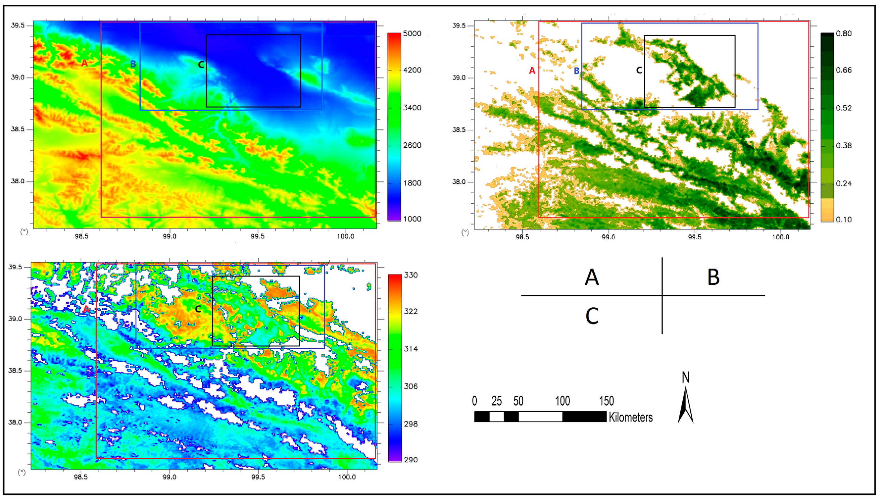
Window A: the largest sub-region with elevations ranging from 1500 m to 5000 m and land cover consisting of forest land, cropland, grassland and unused land (e.g., Gobi and desert);

-

Window B: the intermediate sub-region, which encompasses the middle reaches of the Heihe River basin with elevations from 1500 m to 2180 m and consist of cropland and unused land;

-

Window C: the target area to be evaluated, which is flat with elevations ranging from 1500 m to 1730 m and land cover is dominated by cropland, located in the middle reach of Heihe River basin.

The sub-region C in Figure 3 covering mainly part of the middle reach of the Heihe River Basin was chosen as the target area to evaluate the RS-PT method. The pixel-wise ET is calculated for this target area using RS-PT method (Equations (1), (2) and (3)) with the coefficient ϕ calculated from LST-Fc feature space constructed from the three different image windows A, B and C. Figure 4 shows the spatial distribution of the coefficient ϕ and the corresponding LST-Fc feature space. The dry/wet boundaries, determined using statistical method, are also given in each diagram.

Figure 3. The spatial distribution of (A) Digital Elevation Model (DEM) (unit: m); (B) Fc and (C) LST (unit: K) in the entire study area. The three rectangles (A), (B), and (C) indicate the nested windows to build the LST-Fc feature space.

Figure 3. The spatial distribution of (A) Digital Elevation Model (DEM) (unit: m); (B) Fc and (C) LST (unit: K) in the entire study area. The three rectangles (A), (B), and (C) indicate the nested windows to build the LST-Fc feature space.

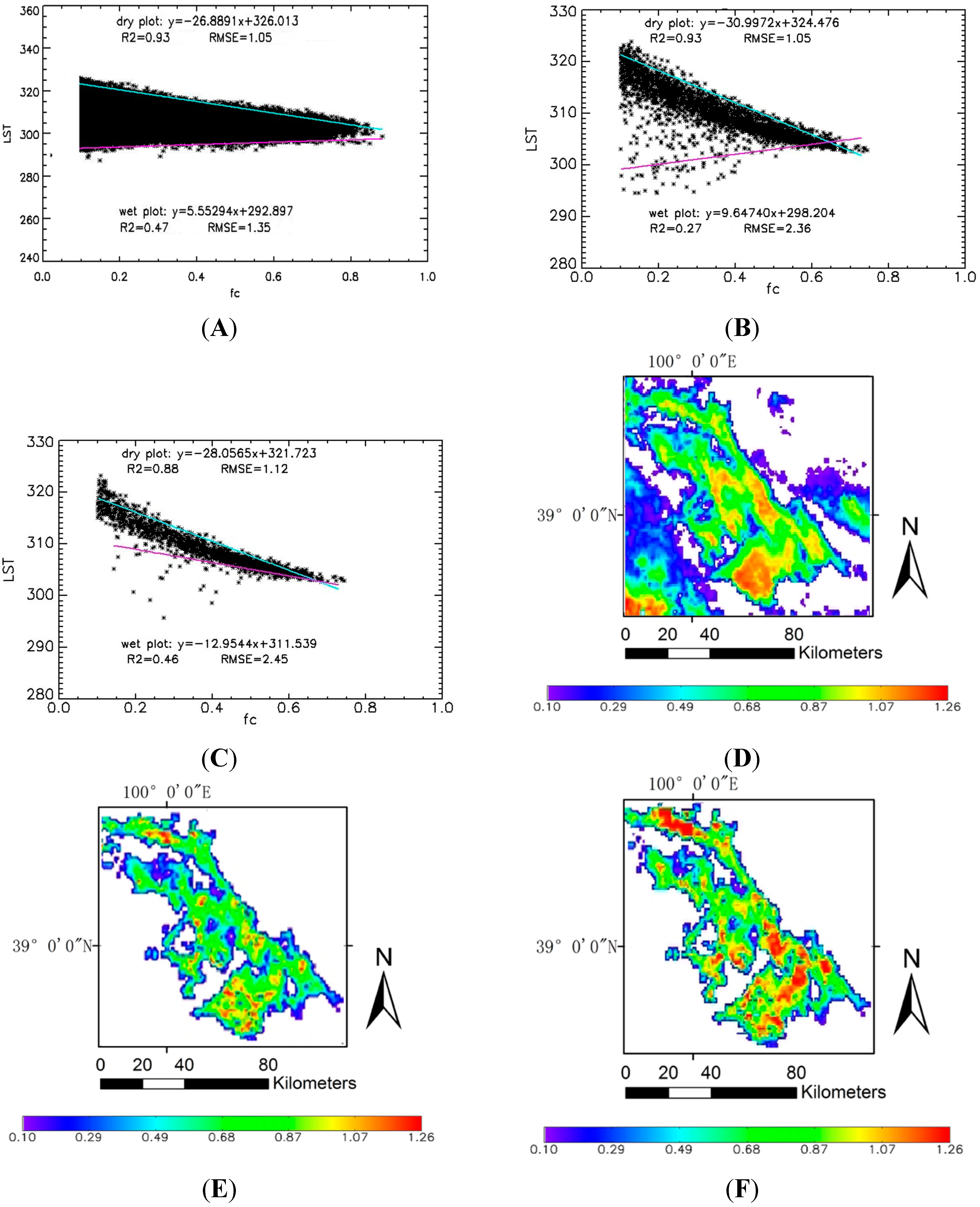
The LST-Fc diagram of region A is nearly a standard triangle feature space (Figure 4A). Due to the elevation effect, the LST in mountain area is lower than that of cropland in the study area as shown in Figure 3C. As a consequence, many wet pixels with low LST along the wet edge might not necessarily be well-watered pixels but can be pixels at higher elevations. Although the shape of the LST-Fc feature space in Figure 4A seems to be perfect, the mis-defined well-watered pixels in the mountainous areas may cause errors in calculating the coefficient ϕ.

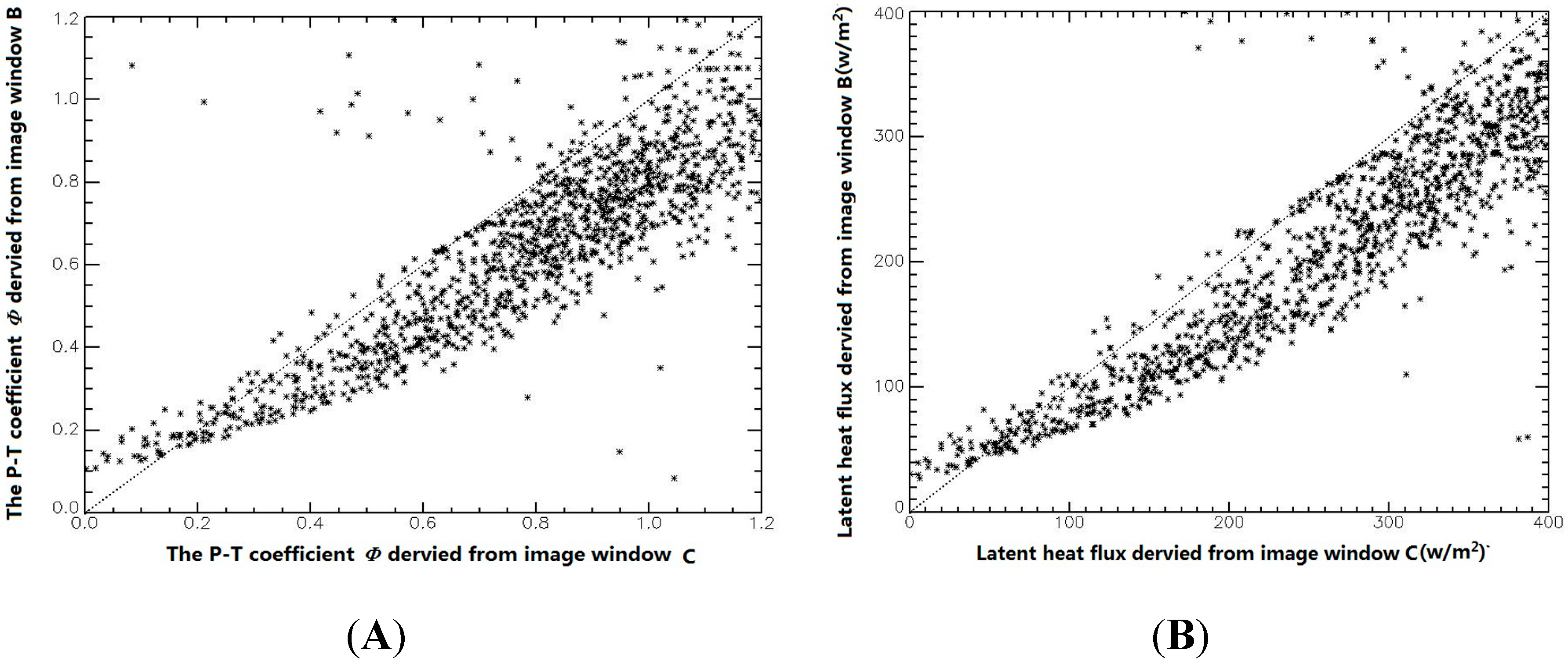
For the areas B and C, to remove the elevation effect, pixels with elevations greater than 1750 m were first masked out before constructing the LST-Fc diagrams. As shown in Figure 4B,C, the shapes of the LST-Fc diagrams from sub-regions B and C are obviously different. We used the scatter plot to evaluate the effect of study area size on the coefficient ϕ estimation. The P-T coefficient ϕ based on the image windows B and C as well as the resulting ET are compared and presented in Figure 5.

As shown in Figure 5, the coefficient ϕ derived from LST-Fc space of window C is larger than that from the LST-Fc space of window B, with mean difference of 0.13 and a standard deviation (STD) of 0.27 for the difference. The overestimation is more obvious for the pixels with higher ϕ values. For the pixels with ϕ < 0.2, i.e., near to the dry bare soil, the value ϕ from area B is lower than that derived from area C. The comparison of latent heat flux in Figure 5B gives similar result: the latent heat flux estimated using LST-Fc space of window C is larger than that from LST-Fc space of window B with a mean discrepancy of 69.5 W/m² and STD of 114.7 W/m². In theory, the value of ϕ for a given pixel depends on the relative position of the pixel between the dry and wet edges in the LST-Fc feature space. With different spatial coverage of the study area, the respective statistical boundaries also change in the varying LST-Fc feature space (e.g., Figure 4B,C). Thus, the relative position of any pixel changes with the varying wet or dry edge. This leads to a varying value ϕ with the change of size and location of the windows that determine the LST-Fc feature space as shown in Figure 4. From the above analysis, we can draw the conclusion that the difference both in the LST-Fc feature spaces and the coefficient ϕ between window B and window C is completely caused by the different size of the two windows and a resulting different range of land surface properties (e.g., Fc, LST and soil moisture).

Figure 4. The LST-Fc feature space constructed respectively using: (A) image window A; (B) image window B; and (C) image window C in Figure 3; (D,E,F)—the coefficient ϕ of the target area estimated using the three windows A, B and C in Figure 3 for LST-Fc feature space, respectively.

Figure 4. The LST-Fc feature space constructed respectively using: (A) image window A; (B) image window B; and (C) image window C in Figure 3; (D,E,F)—the coefficient ϕ of the target area estimated using the three windows A, B and C in Figure 3 for LST-Fc feature space, respectively.

Figure 5. Comparison of estimated values for target area (window C) using LST-Fc feature space constructed from windows B and C respectively: (A) coefficient ϕ; and (B) latent heat flux.

Figure 5. Comparison of estimated values for target area (window C) using LST-Fc feature space constructed from windows B and C respectively: (A) coefficient ϕ; and (B) latent heat flux.

It should be noted that the size of image window C is relative small compared with image window B, thus the range of soil moisture is narrow and the number of soil pixels with lower LST in window C is rather rare. Therefore, it is questionable that the wet boundary can be derived correctly from the LST-Fc diagram feature space constructed using the image window C.

The results show that the LST-Fc diagram does not only depend on the size of the area to build the LST-Fc feature space, but also on the ranges of the land surface Fc and soil moisture found in the area. The varying size of the sample window may lead to varying LST-Fc scatter plots and dry/wet boundaries, in turn, affect the coefficient ϕ. In addition, the area to construct the LST-Fc diagram should meet the precondition, which is to have a relatively small variation in elevation.

4.2. Evaluation of RS-PT Method with High Resolution Data from WiDAS

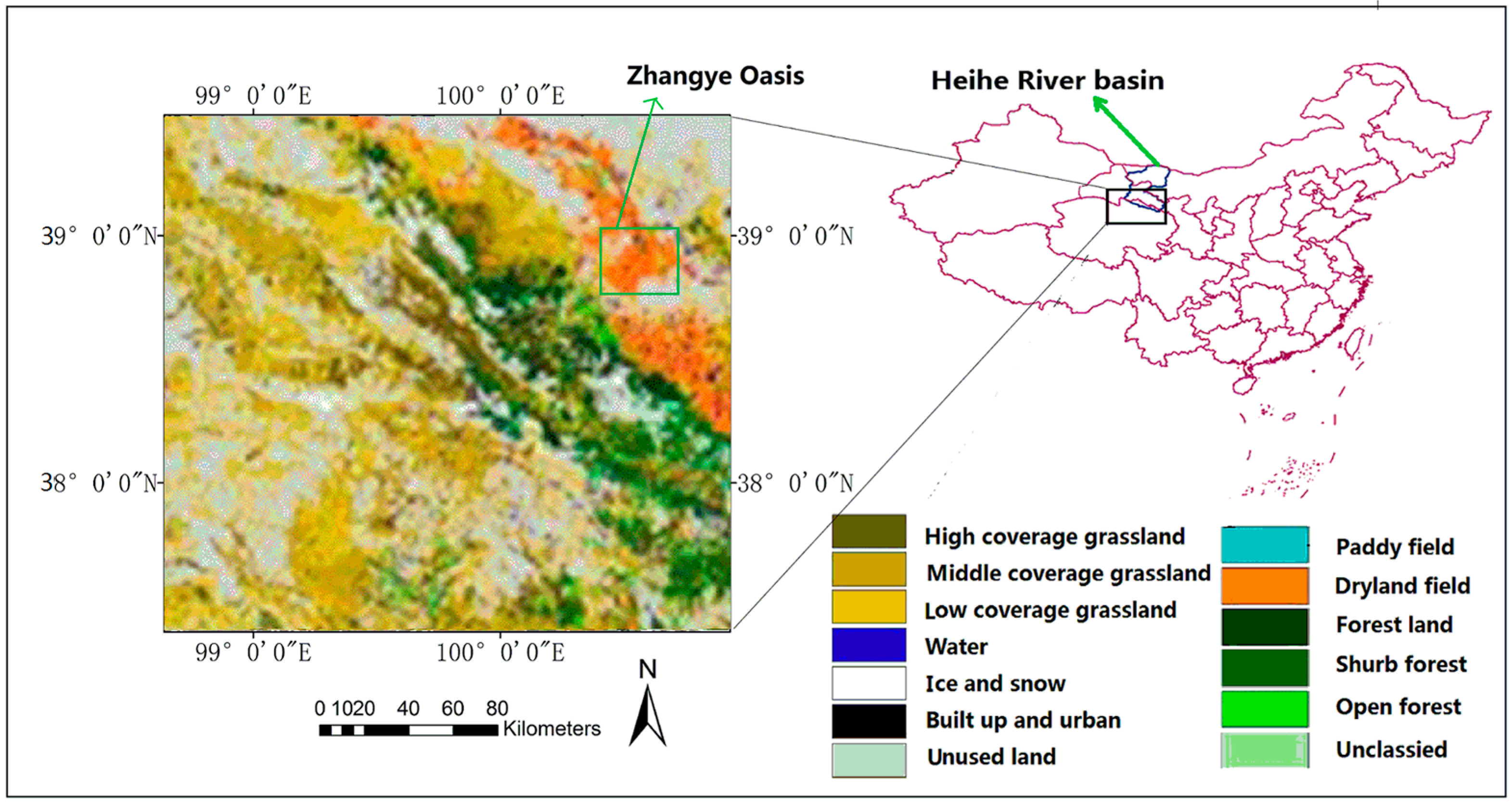
As the WiDSA is an airborne remote sensing sensor, the spatial coverage of WiDSA image is much smaller compared with that of satellite AATSR image. In this study, the image of WiDAS covers part of Zhangye Oasis, which is dominated by irrigated maize crops with village buildings and roads distributed in between. The WiDAS image was acquired on the same day during growing season, i.e., 7 July 2008.

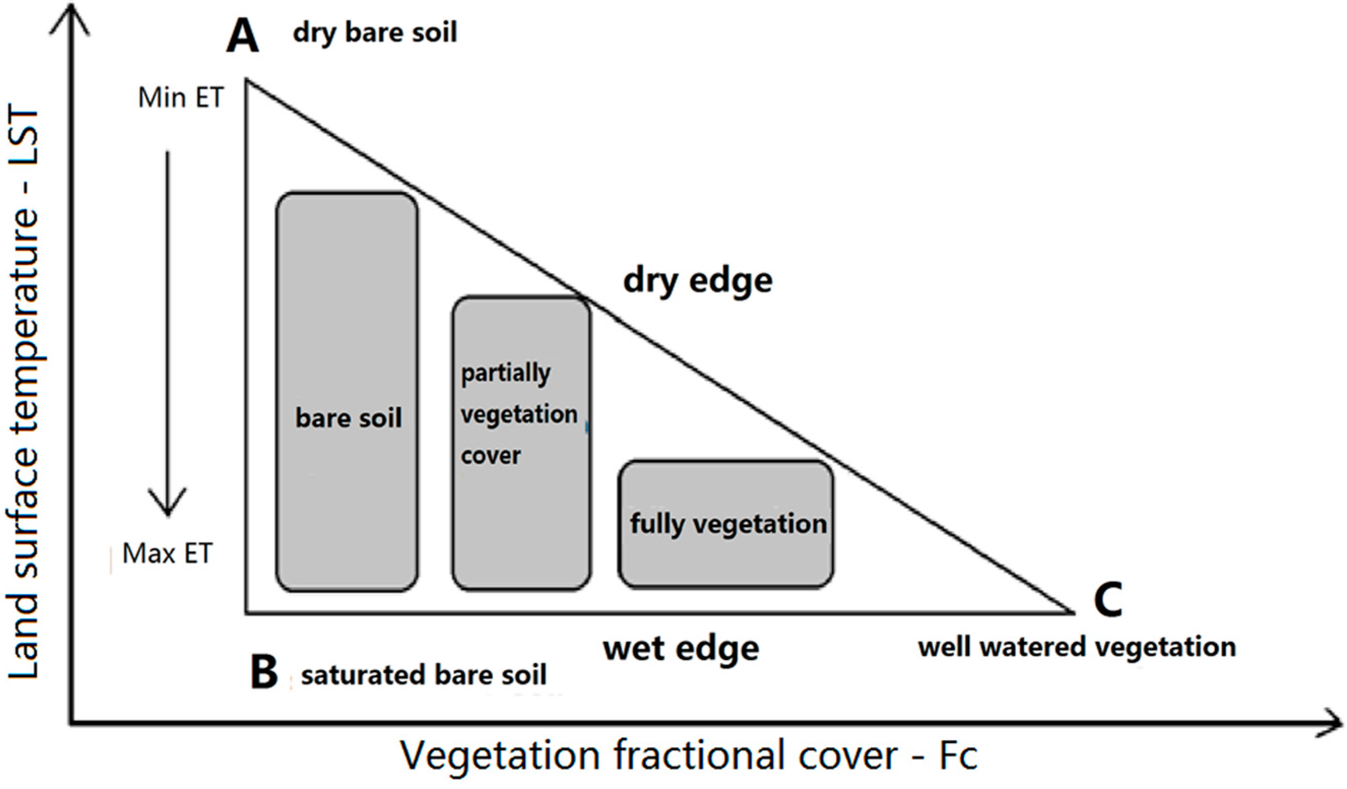
Because the spatial resolution of WiDAS image is very high, the non-vegetated area (e.g., house roof, roads, pool, etc.) could be easily identified by visualization. As the pixels of water body are characterized by lower LST and strong evaporation, they can be treated as well-watered “soil” pixels. The pixels of impervious surface have a heating effect through absorbing solar energy rapidly. Due to the lower heat capacity with respect to that of bare soil, the temperature of an impervious surface is usually higher than that of a dry bare soil. At the coarse resolution of an AATSR image, the influence of impervious surface pixels on the LST-Fc diagram is not obvious due to the mixture of different elements in a pixel. At high resolution, however, these pixels of impervious surfaces appear explicitly around point A in Figure 1, corresponding to the maximum LST and minimal Fc. These pixels do not satisfy the definition of the dry pixel in Section 2.1. We refer to these pixels with impervious surfaces as “erroneous dry pixels” (fake dry pixels) and the derived dry edge based on the fake dry pixels is referred to as an erroneous dry edge (fake dry edge).

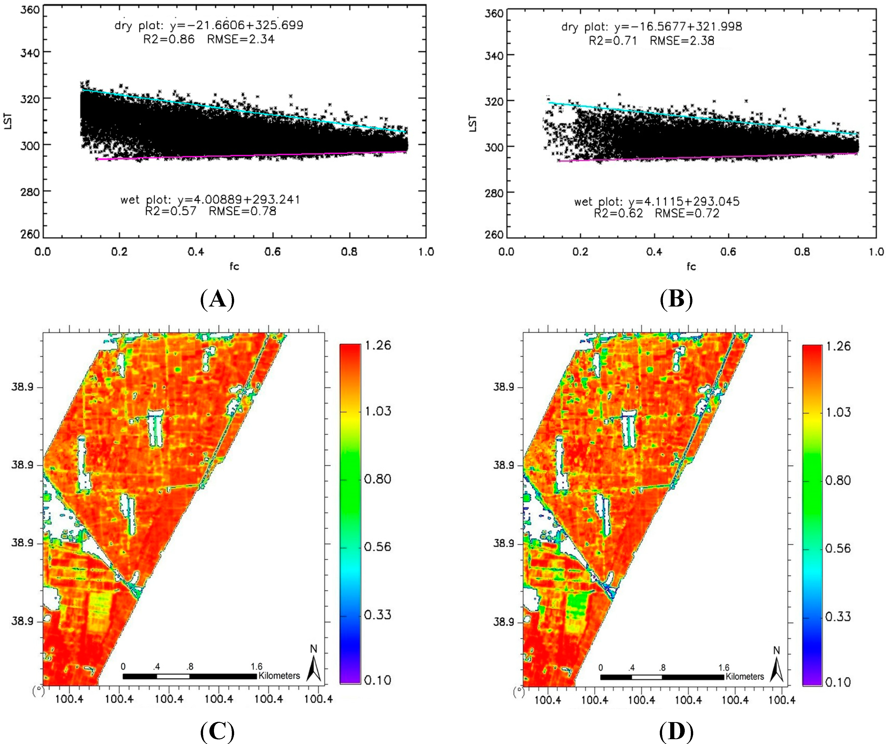
The results of the estimated ϕ and LST-Fc feature space measured by WiDAS are shown in Figure 6. The LST-Fc feature space in Figure 6A, referred to as original feature space, is the result constructed normally with all pixels in the image. The feature space in Figure 6B corresponds to the refined result obtained using refined feature space in Figure 6D, that is constructed with the residual pixels after removing the erroneous dry pixels.

Figure 6. The LST-Fc feature space constructed respectively by: (A) using the WiDAS image, denoted as original feature space; (B) using WiDAS image data without erroneous dry pixels, denoted as refined feature space. (C,D) the results of coefficient ϕ estimated from LST-Fc feature space (A) and (B) respectively.

Figure 6. The LST-Fc feature space constructed respectively by: (A) using the WiDAS image, denoted as original feature space; (B) using WiDAS image data without erroneous dry pixels, denoted as refined feature space. (C,D) the results of coefficient ϕ estimated from LST-Fc feature space (A) and (B) respectively.

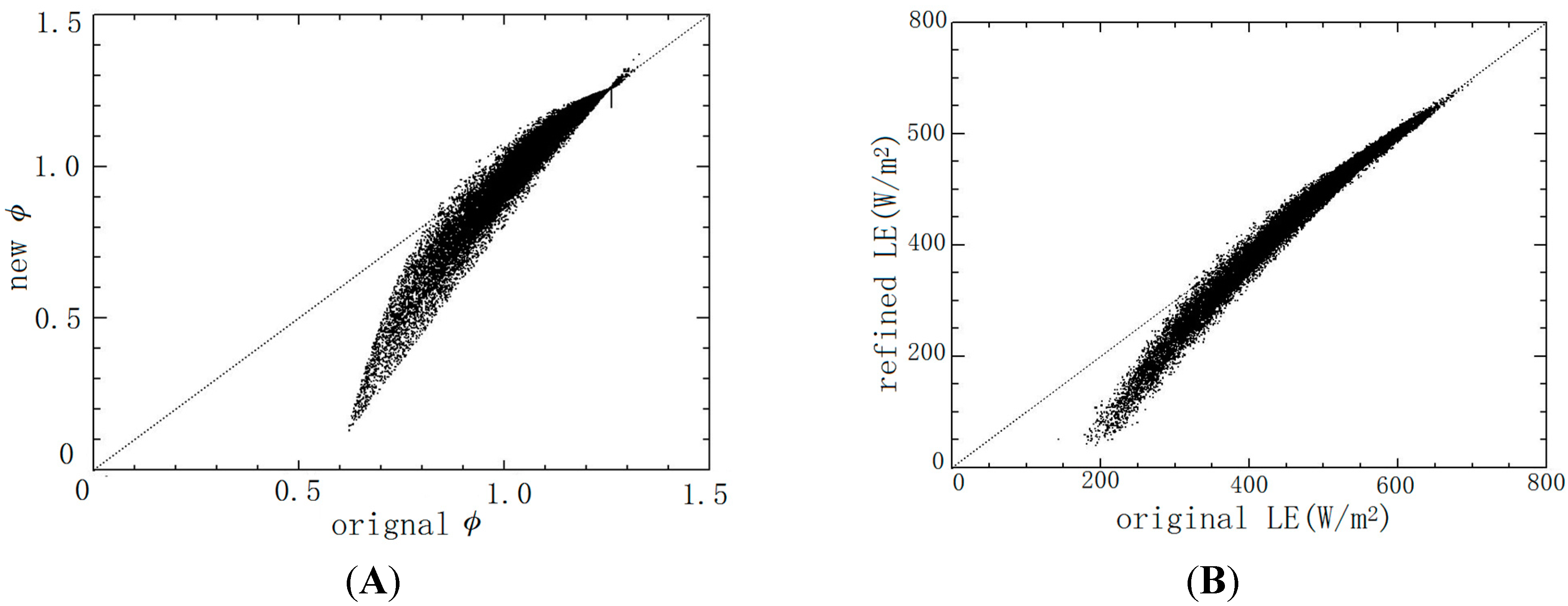
The maize was irrigated several times during the growing season. The irrigation schedule was not the same for different maize fields, this result in a relative broad range of the soil moisture for vegetation-covered pixels over this area. As a consequence, the diagram of WiDAS shows a typical trapezoid shape (Figure 6A,B). The comparison between the original feature space (Figure 6A) and the refined feature space (Figure 6B) shows that the position of the erroneous dry edge is higher than that of the real dry edge in the LST-Fc diagram. This would cause errors in the calculation of P-T coefficient ϕ and ET. Analogous to Figure 5, the scatterplots of original and refined results (Figure 7) were used to evaluate the influence of erroneous dry pixels on the estimation of the P-T coefficient ϕ and of ET. It is obvious that the values of coefficient ϕ derived from the original feature space are higher than that from the refined feature space due to its erroneous dry edge, and it is more obvious for the pixels with relatively lower ϕ. The difference in coefficient ϕ between the original feature space (Figure 6C) and the refined one (Figure 6D) ranges from −0.01 to 0.46 with a mean of 0.02 and STD of 0.05, and the corresponding difference in LE varies from −35 W/m² to 167 W/m² with a mean of 15.36 W/m² and a STD of 23.65 W/m². The results in Figure 7 demonstrate that the erroneous dry pixels cause an overestimation of both the coefficient ϕ and of the latent heat flux.

Figure 7. Comparison of original and refined result obtained from original and refined feature space: (A) for coefficient ϕ, and (B) for latent heat flux.

Figure 7. Comparison of original and refined result obtained from original and refined feature space: (A) for coefficient ϕ, and (B) for latent heat flux.

4.3. Assessment of the RS-PT Boundaries by SEBI

The analysis in the previous section shows that the dry/wet boundaries derived from LST-Fc feature space have significant impact on the accuracy of LE estimates. In practice, we believe that the dry/wet boundaries derived from LST-Fc feature space are reasonable if the study area covers the full range of soil moisture and Fc conditions according to the assumption that the dry/wet boundaries determined by regression in the LST-Fc feature space are very close to the theoretical values (see Section 2). Therefore, we need to assess whether the dry/wet boundaries derived from the LST-VI feature space are reasonable and accurate.

In order to investigate the uncertainty associated with the statistical dry/wet boundaries in LST-Fc feature space, the T_s,d and T_s,w calculated by the SEBI model are used to investigate the position of the theoretical dry/wet boundaries. The results are presented in Figure 8. In the LST-Fc feature space, there is only one pair of values T_s,d and T_s,w for all the pixels at the same Fc value, that are on the dry/wet boundaries, respectively. However, according to the SEBI concept, the T_s,d and T_s,w are defined for each pixel, say pixel-dependent. Particularly, difference in aerodynamic resistance will also lead to different dry and wet edges for the same Fc value. That means, for each pixel there would be a corresponding T_s,d and T_s,w. That is the reason why the scatter plots of the Fc and T_s,d do not form a straight line but rather an area as shown in Figure 8, as do the scatter points of Fc and T_s,w.

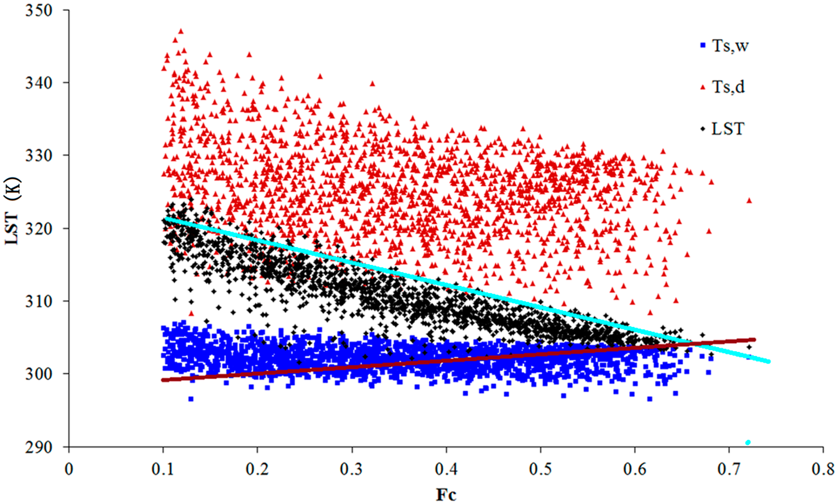
Figure 8. Comparison between the position of theoretical dry/wet pixels from SEBI and the dry/wet boundaries derived from LST-Fc diagram using the moderate resolution AATSR image Window B. Red points represent the T_s,d and blue points represent the T_s,w. The cyan line indicates the dry edge and purple line indicates the wet edge derived by from LST-Fc feature space.

Figure 8. Comparison between the position of theoretical dry/wet pixels from SEBI and the dry/wet boundaries derived from LST-Fc diagram using the moderate resolution AATSR image Window B. Red points represent the T_s,d and blue points represent the T_s,w. The cyan line indicates the dry edge and purple line indicates the wet edge derived by from LST-Fc feature space.

Comparing the cluster of the theoretical (SEBI) wet pixels and the position of RS-PT wet edge in Figure 8, the latter seems reasonable. However, there is a significant difference between the feature-space dry edge and the cluster of the theoretical (SEBI) dry pixels (Figure 8). The feature-space dry edge is much lower than the theoretical (SEBI) dry edge. Similar to the coefficient ϕ, the value of Λ_r depends on the relative position of the pixel value of surface temperature between the two extremes T_s,d and T_s,w in the LST-Fc scatter plot. 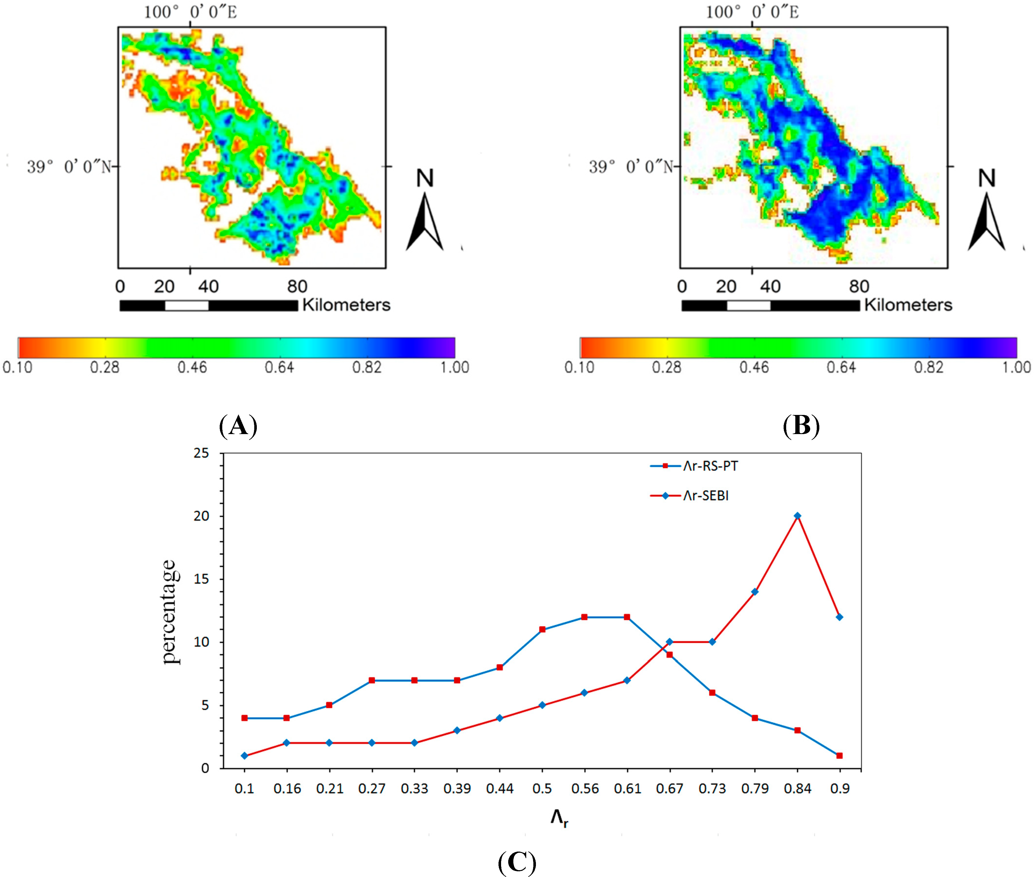As presented in Figure 8, the dry edge of the LST-Fc feature space is lower than the theoretical (SEBI) T_{s, d}, this is to say that Λ_r derived from the LST-Fc feature space would be lower than that deduced from SEBI. The spatial pattern and frequency curves of Λ_r derived from SEBI and RS-PT method over the target area are shown in Figure 9, demonstrating that, compared to SEBI, the RS-PT method underestimates surface wetness (i.e., smaller Λ_r) for most pixels in Zhangye Oasis. The mean discrepancy of Λ_r between SEBI and RS-PT is 0.11 with a STD of 0.32. The results in Figure 9 suggest that there are large uncertainties associated with the statistical boundaries from the LST-Fc feature space.

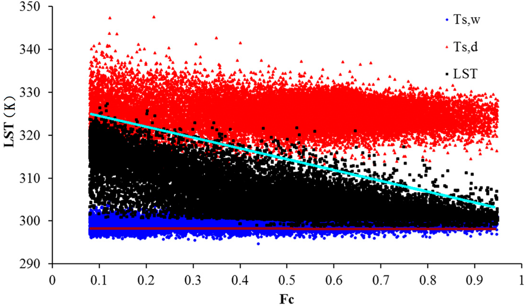
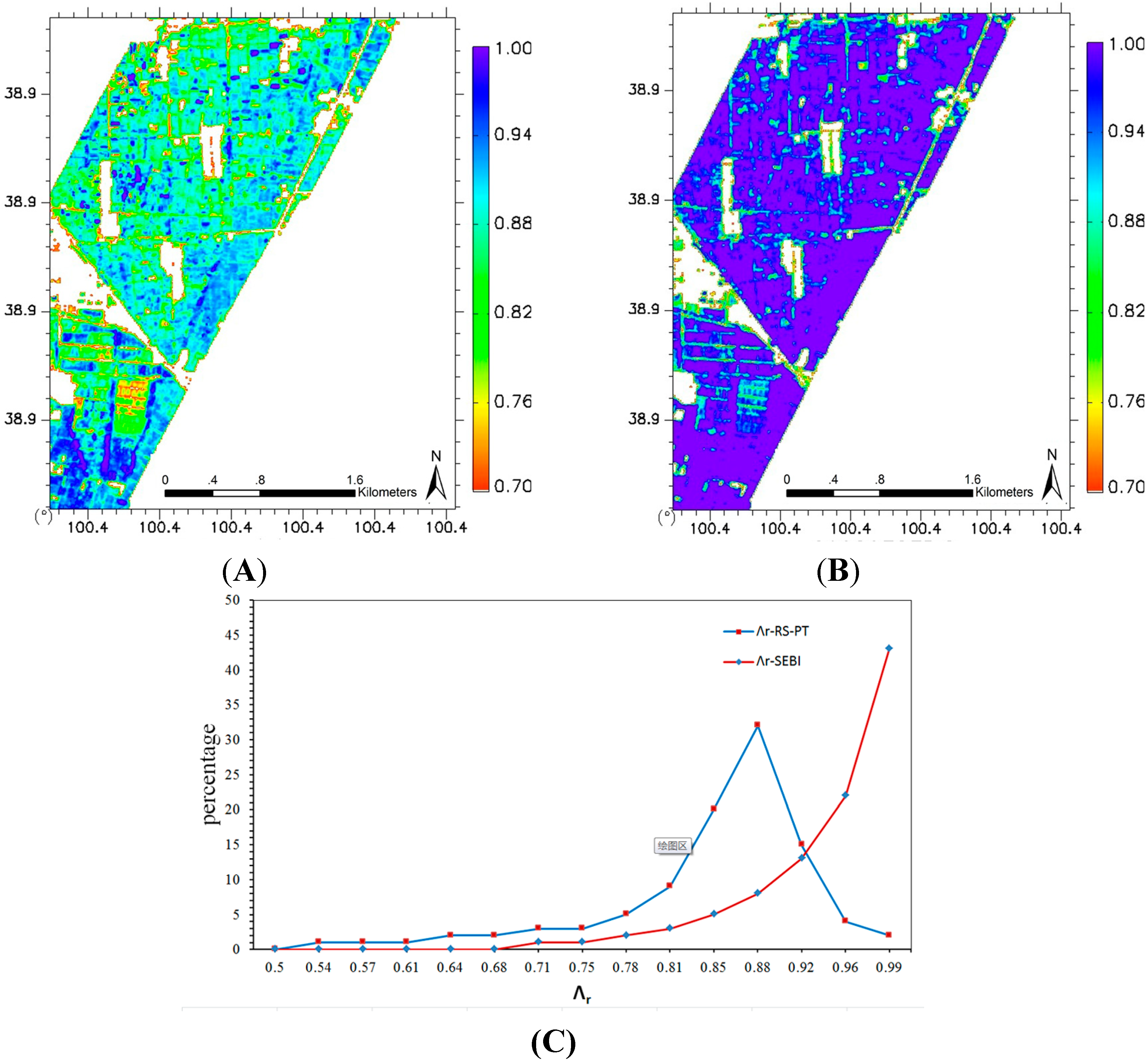
We also derived the theoretical dry/wet pixels for the WiDAS image Window B as shown in Figure 10. As described in Section 4.2, there is abundant irrigation to the maize fields in the growing season. For this reason, there should be many farmland pixels evaporating at potential ET on 7 July 2008. Therefore, the wet edge derived from the RS-PT method using LST-Fc feature space is very close to the theoretical T_s,w (Figure 10). However, the feature-space dry edge is still far from the theoretical (SEBI) dry edge. The comparison of Λ_r derived from SEBI and RS-PT is shown in Figure 11. Compared to Λ_r calculated from SEBI, the Λ_r from the RS-PT method is underestimated by 0.13 with a STD of 0.04. That is because the feature space dry edge is lower than the theoretical (SEBI) dry edge (Figure 10), as a consequence, the Λ_r derived from RS-PT method is lower than that from SEBI over the WiDAS image.

Figure 9. The spatial pattern and frequency curves of Λ_r derived from different methods over the Zhangye Oasis, using the same data as in Figure 8: (A) Λ_r is the result from the statistical dry/wet boundaries based on LST-Fc feature space (Λ_r-RS-PT); (B) Λ_r is calculated based on SEBI (Λ_r-SEBI); and (C) the frequency curves of Λ_r for (A) and (B).

Figure 9. The spatial pattern and frequency curves of Λ_r derived from different methods over the Zhangye Oasis, using the same data as in Figure 8: (A) Λ_r is the result from the statistical dry/wet boundaries based on LST-Fc feature space (Λ_r-RS-PT); (B) Λ_r is calculated based on SEBI (Λ_r-SEBI); and (C) the frequency curves of Λ_r for (A) and (B).

Figure 10. Comparison between the position of theoretical dry/wet boundaries (pixels) from SEBI and the dry/wet boundaries derived from LST-Fc diagram using the high resolution WiDAS image. The labels are identical to those in Figure 8.

Figure 10. Comparison between the position of theoretical dry/wet boundaries (pixels) from SEBI and the dry/wet boundaries derived from LST-Fc diagram using the high resolution WiDAS image. The labels are identical to those in Figure 8.

Figure 11. The spatial pattern and frequency curves of Λ_r from different methods using WiDAS data over Zhangye Oasis on 7 July 2008: (A) Λ_r is obtained using the LST-Fc feature-space (Λ_r_RS-PT); (B) Λ_r_SEBI is obtained based on SEBI (Λ_r-SEBI); and (C) the frequency curves of (A) and (B).

Figure 11. The spatial pattern and frequency curves of Λ_r from different methods using WiDAS data over Zhangye Oasis on 7 July 2008: (A) Λ_r is obtained using the LST-Fc feature-space (Λ_r_RS-PT); (B) Λ_r_SEBI is obtained based on SEBI (Λ_r-SEBI); and (C) the frequency curves of (A) and (B).

Note that the Λ_r derived from RS-PT shows quasi Gaussian distribution but the SEBI-estimated Λ_r show asymmetric distribution peaked around 0.56 in the frequency curves (Figure 9C). The main reason for this is that the Λ_r associated with parameter ϕ derived from RS-PT is calculated using interpolation between 0 and 1; on the contrary the SEBI-estimated Λ_r completely depends on the environmental situation for each pixel. Considering the effect of advection on the oasis, which may cause the failure of energy balance closure, the ground-measured Λ_r without energy balance closure correction was adopted in current study. The ground-measured Λ_r from eddy covariance (EC) measurements at the Yingke station was obtained as reference value for the maize field in the whole study area [30]. Since it was the growing season of maize in July, the Λ_r value reached 0.97 at the sensor overpass time in current study. Therefore, it is reasonable that the value of the SEBI-estimated Λ_r = 0.96 for crop pixels.

From the analysis in Section 4.2, the erroneous dry points would lead to higher dry edge. However, compared with the theoretical dry pixels in Figure 10, the erroneous dry pixels are closer to the theoretical dry edge in this case. Therefore, the original feature space in Figure 6B is not reasonable, but may nevertheless be closer to the actual value than the refined feature space for this case. This apparent contradiction is still caused by the limitation of the method for the dry/wet boundaries depending on LST-Fc scatter plot in the RS-PT model.

4.4. Summary of the Issues about RS-PT Method

4.4.1. Issues about the Uncertainty in RS-PT Application

The varying size of the area of interest used to construct the LST-Fc feature space causes the different LST-Fc feature spaces and dry/wet boundaries, and therefore leading to uncertainties in the coefficient ϕ and ET estimates. The low resolution and large spatial coverage AATSR image captured a broader range of soil moisture and vegetation cover, which is essential to construct a reasonable feature space. However, the inhomogeneous atmospheric conditions and the difference of elevation over AATSR image may cause errors in the estimate on ET. Contrarily, the small area covered by the airborne WiDAS can be safely assumed to have homogenous atmospheric conditions and small elevation variation, but the range of soil wetness and Fc is likely to be too narrow. The latter may cause errors in the estimate of the dry and wet edges using the LST-Fc feature space method.

4.4.2. Issues about the Uncertainty on the Dry/Wet Boundaries

From the analysis in Section 4.3, we may conclude that the assumptions and preconditions must be met to derive reasonable wet and dry boundaries from LST-Fc feature space in the RS-PT method. The impact of the erroneous dry pixels must be must be paid enough attentions in application, particularly when the high-resolution images used include urban areas. Compared with the theoretical dry/wet boundaries from SEBI, it is relative difficult to get correct and accurate dry/wet boundaries just using the LST-Fc feature space in general, especially for the dry edge. Taking into account the effect of domain size effect on the wet and dry boundaries in the LST-Fc feature space in practical applications, one should pay much attention to the accuracy of the dry/wet boundaries when applying the RS-PT method for ET estimation.

5. Conclusions

This study evaluates the remote sensing-based Priestley-Taylor method (RS-PT method) over an arid and semi-arid region in northwest China from a comprehensive view, including the preconditions of this methods and the influence of domain size as well as high resolution scale effects, and examines the accuracy of dry/wet boundaries from land surface temperature-fractional vegetation cover (LST-Fc) feature space by using theoretical dry/wet boundaries. The uncertainties of the RS-PT method caused by domain size are analyzed using the moderate-resolution remotely sensed data from the Advanced Along-Track Scanning Radiometer (AATSR). The results show that when the research area is heterogeneous surface with the mountainous areas, the pixel along the wet edge might not necessarily be well-watered pixels but the pixels at higher elevations. The mean difference for Priestley-Taylor (P-T) coefficient (ϕ) estimates resulted from different domain sizes is 0.13 with a standard deviation (STD) of 0.27 and is 69.5 W/m² with a STD of 114 W/m² for latent heat flux (LE) estimates. When the high resolution images from airborne Wide-angle Infrared Dual-mode line/area Array Scanner (WiDAS) are used, it can be concluded that impervious surfaces leading to the erroneous dry pixels strongly affected the dry edge and resulted in the mean difference of 0.02 with a STD of 0.05 for ϕ estimates and of 15.36 W/m² with a STD of 23.65 W/m² for LE estimates. Therefore, the erroneous dry pixels from impervious surfaces must be paid enough attentions when the high-resolution images are used. The statistical dry/wet boundaries in LST-Fc feature space are also compared with the theoretical dry/wet boundaries derived from the physically based Surface Energy Balance Index (SEBI) model. In general, the statistical feature-space dry edge is lower than the SEBI-based theoretical dry edge, and the RS-PT method underestimates relative evaporative fraction (Λ_r) by ~0.11 compared with the SEBI-estimated values.

The applicability of the RS-PT method is restricted by the pre-conditions of homogeneous atmospheric conditions and a large range of land surface cover and soil moisture conditions. ET estimates from the RS-PT method strongly depend on the size of the area to build the LST- Fc feature space. However, how large the research area is the best scale for constructing LST- Fc feature space is still unclear. This work only analyzed the uncertainties of the LST-Fc method applied to the arid and semi-arid condition. More works need to be done to further quantify the uncertainties associated with dry/wet boundaries in the LST-Fc feature space method over different land cover and climate regions.