1. Introduction
Urban landscapes are extremely complex and heterogeneous. To adequately quantify the heterogeneity of urban land cover, high spatial resolution images are needed. A considerable amount of research has shown that object-based approaches are superior to traditional pixel-based methods in the classification of high spatial resolution data [
1,
2,
3,
4]. Consequently, object-based approaches have been increasingly used for urban land cover classification [
5,
6,
7].
With object-based classification approaches, objects generated from image segmentation can be typically classified using a rule-based procedure (a set of rules) [
8] or using machine learning algorithms (MLA) based on training samples [
1]. While rule-based procedures, which use expert knowledge, have been increasingly used for classification, the majority of the studies have used supervised classifications [
5,
9,
10]. Many different kinds of MLA have been applied for supervised classifications. These algorithms are commonly categorized as parametric and non-parametric classifiers. The two widely-used types of parametric algorithms are the maximum likelihood classifier (MLC) and Bayes classifiers, and the frequently-used non-parametric classifiers include K nearest neighbor (KNN), decision tree (DT) and support vector machine (SVM).
Previous studies have shown that the use of different classifiers may lead to different classification results. Therefore, many studies have been conducted to investigate the effectiveness and efficiency of different classifiers [
11,
12,
13,
14]. However, these studies have been mostly conducted using pixel-based approaches. With the wide use of object-based approaches, there has been an increasing interest in comparing different machine learning classifiers using object-based methods [
5,
9,
15,
16,
17]. When using these machine learning classifiers, we should consider at least four key factors that can dramatically affect the classification accuracy and efficiency. Specifically, these are image segmentation, training sample selection, feature selection and tuning parameter setting [
1,
5]. While the first three factors have been investigated in many previous studies [
16,
18,
19], few studies have investigated the effects of the setting of tuning parameters [
5]. However, setting tuning parameters is the very first step, as well as one of the most important steps to appropriately use these machine learning classifiers. In addition, previous comparison studies of machine learning classifiers have been mostly focused on non-urban areas, such as grasslands, farmlands and coal mine area [
5,
9,
20].
The overall objective of this study is to evaluate the four most frequently used MLAs for urban land cover classification, with an object-based approach, using very high spatial resolution imagery. In particular, we aim to investigate how tuning parameters affect the classification results, especially with different training sample sizes. The four classifiers are: (1) normal Bayes (NB), a parametric algorithm; (2) SVM, a statistical learning algorithm; (3) KNN, an instance-based learning algorithm; and (4) the classification and regression tree (CART) classifier, a commonly-used DT algorithm. The results from this study can provide insights into classifier selection and parameter setting for high resolution urban land cover classification.
2. Study Area and Data
2.1. Study Site
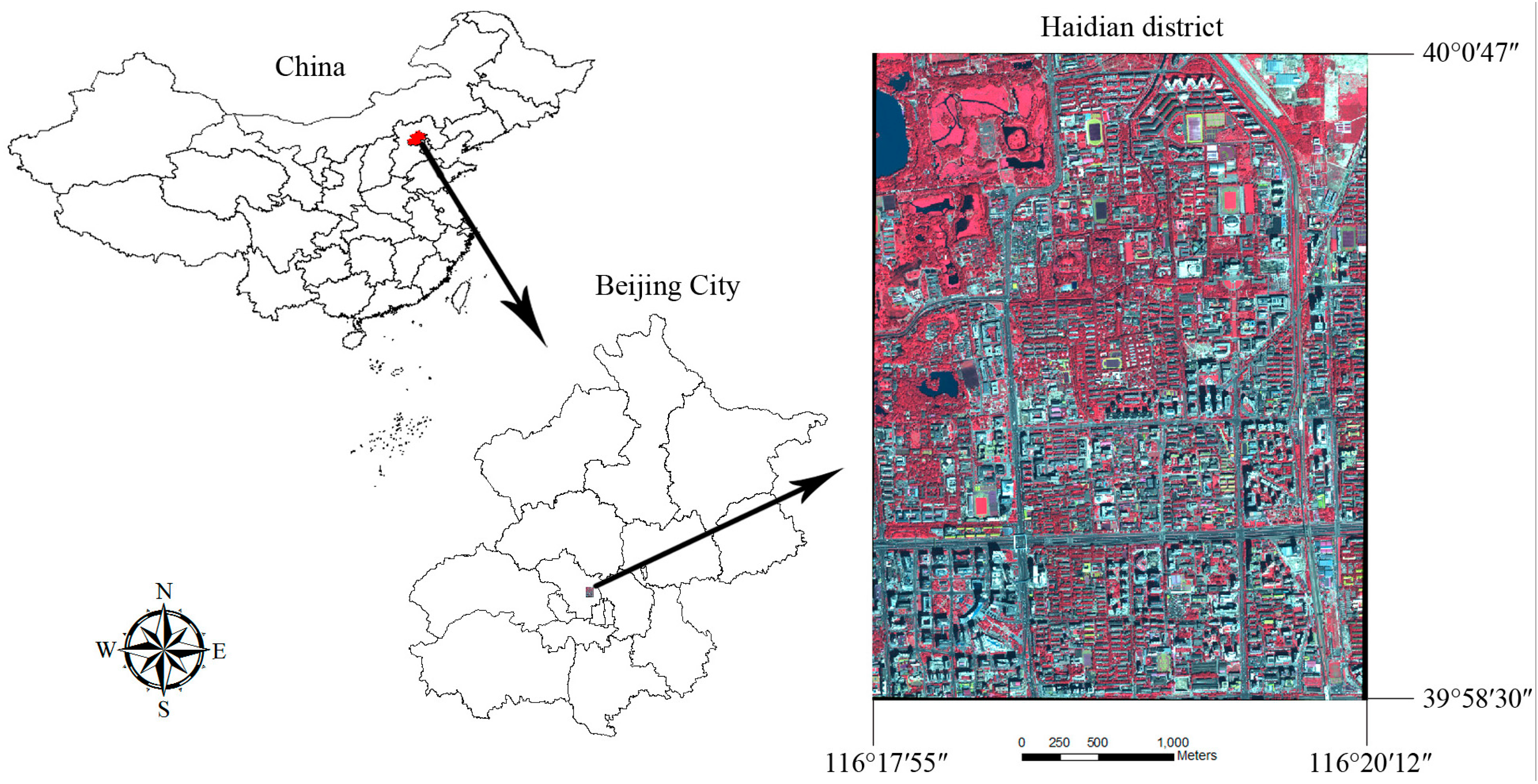
The study site is an urban area located in the Haidian District of Beijing, China, between latitudes 39°58′30″ and 40°0′47″ and longitudes 116°17′55″ and 116°20′12″. The study area is a complex urban area with many land use types, including parks, universities, construction sites and residential areas. Land cover types are mainly impervious surface, vegetation cover, bare soil and water, which are typical in urban areas. The dominant land cover in parks is vegetation and water, while in the universities and the residential areas, the primary land cover is impervious surfaces, mixed with dispersed small patches of greenspace. Bare soil is the dominant land cover type in construction sites (
Figure 1).
Figure 1.
The study area, an urban area located in the Haidian District of Beijing, China.
Figure 1.
The study area, an urban area located in the Haidian District of Beijing, China.
Table 1.
WorldView-2 specifications.
Table 1.
WorldView-2 specifications.
| Sensor Bands | Spectral Range | Spatial Resolution |
|---|
| Panchromatic | 450–800 nm | 0.46 m |
| Coastal | 400–450 nm | 1.85 m |
| Blue | 450–510 nm | 1.85 m |
| Green | 510–580 nm | 1.85 m |
| Yellow | 585–625 nm | 1.85 m |
| Red | 630–690 nm | 1.85 m |
| Red Edge | 705–745 nm | 1.85 m |
| Near-IR1 | 770–895 nm | 1.85 m |
| Near-IR2 | 860–1040 nm | 1.85 m |
2.2. Data
We used WorldView-2 satellite imagery, acquired on 14 September 2012, for land cover classification. WorldView-2, launched in October 2009, is the first high resolution 8-band multispectral commercial satellite (
Table 1). The dynamic range is 11 bits. To take advantage of both the high spatial resolution and multispectral features of WorldView-2, a principal component merging algorithm was used to merge the multispectral bands and panchromatic band into a new multispectral image with 0.5-m spatial resolution using ERDAS
TM 10. Four land cover types were identified for the study area: (1) impervious surfaces; (2) vegetation; (3) water; and (4) bare soil. Impervious surfaces were mainly roads and building roofs. Vegetation included trees and grass. Water mostly occurred in parks and bare soil in construction sites. Shadows from buildings and trees are common in very high resolution images of urban areas. Therefore, we included the shadow class and separated shadows from unshaded land cover types [
21].
3. Methods
The object-based classification procedure includes image segmentation, training sample selection, classification feature selection, tuning parameter setting and, finally, algorithm execution. We first segmented the image into land cover segments and then chose a certain amount of segments of different land cover types as training samples. After comparing the training sample characteristics of different land cover types, we selected certain object features for classification. Finally, we adjusted the tuning parameters of different classifiers to generate high classification accuracy. For all four classifiers, we used the same procedure for image segmentation and the selection of training samples and classification features. The optimal setting of tuning parameters, however, were determined separately for each classifier. Following the classifications, object-based accuracy assessment was applied to evaluate different classifiers.
3.1. Image Segmentation
Many approaches to image segmentation have been applied to land cover classification [
8]. Here, we used the multi-resolution segmentation approach embedded in Trimble eCognition. The multi-resolution segmentation algorithm is a bottom-up approach that consecutively merges pixels or existing image objects into larger ones, based on the criteria of relative homogeneity. Scale, shape and compactness parameters can be customized to define the size and shape of segmented objects. The scale parameter defines the maximum standard deviation of the homogeneity criteria in regard to the weighted image layers for generating image objects [
22]. In general, the greater the scale value, the larger the size of objects and the higher the heterogeneity. In this study, we selected the scale parameters using an iterative “trial and error” approach [
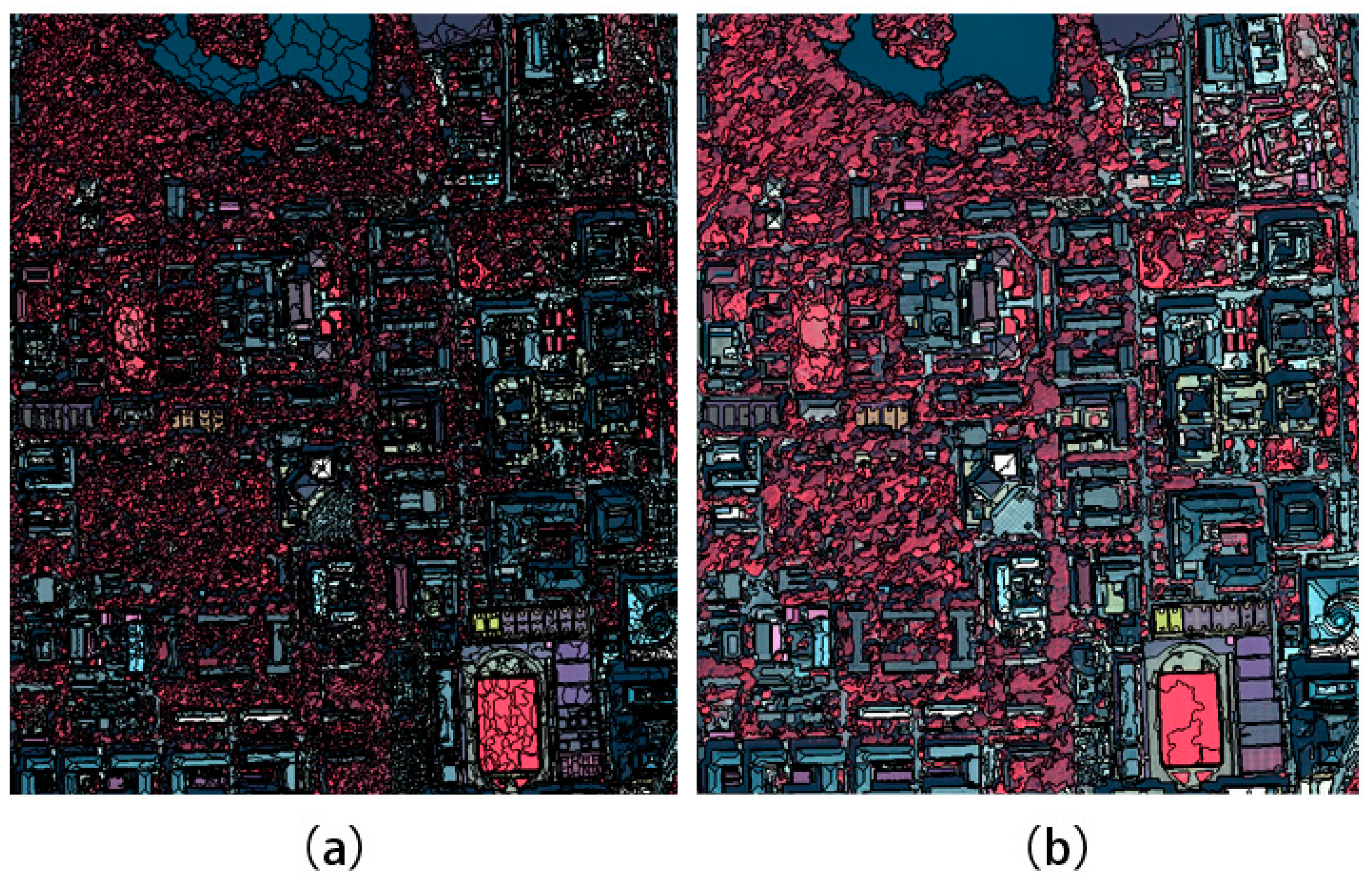
8]. Two object levels were created with the scale value setting at 30 and 100 (afterwards referred to as Level 1 and Level 2), respectively. The relatively small value of 30 was set to create homogeneous segments and, thus, to avoid the influence of mixed land cover objects. The coarser value of 100 was set to generate larger segments that depict a larger land cover of interest (
Figure 2). Through the trial-and-error approach and experience from previous studies [
1,
10], we assigned both object levels with the color weight of 0.9 and the shape weight as 0.1 to generate meaningful objects. The two parameters for compactness and smoothness were set equally as 0.5, based on visual inspection of the segmentation results. Equal weight was set for each of the 8 original image layers for segmentation. The number of segmented objects for Level 1 and Level 2 were 409,024 and 55,502, respectively.
Figure 2.
(a) Segmented image objects in Level 1; (b) segmented image objects in Level 2.
Figure 2.
(a) Segmented image objects in Level 1; (b) segmented image objects in Level 2.
3.2. Selection of Training, Testing Samples and Classification Features
There are some basic principles for the selection of training samples for pixel-based classification [
18,
19]. The number of object-based training samples, however, is usually determined based on the researcher’s experience. Using Google Earth, we randomly chose 1500 object samples, 300 for each class, for the classifications and accuracy assessment. These samples were chosen at Level 1 to ensure “pure” objects that contained only one land cover type. We then randomly divided the 1500 object samples into two sets: 1000 as training samples and 500 as testing samples. To investigate the sensitivities of classifiers to the size of training samples, 8 training sample subsets were generated by randomly sampling from the total training sample set. The sizes of the training samples of those subsets were 125, 250, 375, 500, 625, 750, 875 and 1000, respectively. Within a training subset, the numbers of samples for each of the five classes were equal, and thus, the sample numbers of each class within the 8 training sample subsets were 25, 50, 75, 100, 125, 150, 175 and 200, respectively. Likewise, in the testing sample set, there were 100 samples per class.
Following the selection of the training and testing samples, spectral and spatial features of the training samples were selected for land cover classifications. There are more than one hundred object features that could be potentially incorporated into classifications [
5,
9]. Therefore, the selection of optimal object features was determined based on an approach that integrates expert knowledge and quantitative analysis. First, we chose a large number of object features that were frequently used in previous studies [
1,
5]. We then used the feature space optimization tools available in Trimble eCognition, combined with comparisons of the histograms of each feature among five land cover types to determine the selection of optimal object features. Consequently, we selected out 36 object features. These 36 features included 32 features calculated based on the 8 multispectral bands, that is mean value, standard deviation, mean difference to the super-object and standard deviation difference to the super-object of the 8 multispectral bands. In addition, we chose Brightness, Max. diff. (max intensity difference), NDVI (Normalized Difference Vegetation Index) and NDWI (Normalized Difference Water Index) for classifications (
Table 2).
Table 2.
Object features used for classification.
Table 2.
Object features used for classification.
| Object Features | Description |
|---|
| Mean value a | Mean value of a specific band of an image object |
| Standard deviation a | Standard deviation of an image object |
| Mean difference to super-object a | The difference between the mean input layer value of an image object and the mean input layer value of its super-object. Distance of 1. |
| SD difference to super-object a | The difference of the SD input layer value of an image object and the SD input layer value of its super-object. Distance of 1. |
| Brightness | Mean value of the 8 multispectral bands |
| Max. diff. | Max intensity difference of the 8 multispectral bands |
| NDVI | (NIR1 − Red)/(NIR1 + Red) |
| NDWI | (Green − NIR1)/(Green + NIR1) |
3.3. Classifiers and Primary Tuning Parameters
When using CART, KNN and SVM, one of the key steps is to set the tuning parameters, which are different for different classifiers. For each classifier, we tested a series of values for its tuning parameters to determine the optimal parameters, that is by which the classifier generates the highest overall classification accuracy. When comparing different classifiers, we used the classification results under the optimal parameters. In addition, the sensitivity of each classifier was examined using the 8 training sample subsets. The algorithms of the 4 classifiers were based on OpenCV [
23].
DT, first developed by Breiman
et al. (1984) [
24], is a typical non-parametric model used in data mining. We used the classification and regression tree (CART) algorithm, one of the most commonly-used DT in this study. With CART, a tree can be developed in a binary recursive partitioning procedure by splitting the training sample set into subsets based on an attribute value test and then repeating this process on each derived subset. The tree-growing process stops when no further splits are possible for subsets. The maximum depth of the tree is the key tuning parameter in CART, which determines the complexity of the model. In general, a larger depth can build a relatively more complex tree with potentially higher overall classification accuracy. However, too many nodes may also lead to over-fitting of the model. In this study, we tested the value of “maximum depth” from 1 to 20 for all 8 training sample subsets, setting other parameters at the default value (e.g., cross-validation folds and min sample count both set to the default value of 10).
SVM is also a non-parametric algorithm that was first proposed by Vapnik and Chervonenkis (1971) [
25]. With the SVM algorithm, a hyperplane is first built based on the maximum gap of the given training sample sets, and then, it classifies the segmented objects into one of the identified land cover classes (in this study, four classes). To map non-linear decision boundaries into linear ones in a higher dimension, the four most frequently used types of kernel functions in SVM algorithms are linear, polynomial, radial basis function (RBF) and sigmoid kernels [
26]. In this study, we chose the most frequently used RBF kernel, which has been proven superior to other kernels in previous studies [
5,
14]. The RBF kernel has two important tuning parameters—“cost” (C) and gamma—which can affect the overall classification accuracy [
27]. A large C value may create an over-fitted model, while adjusting the gamma will influence the shape of the separating hyperplane. The optimal value of parameters C and gamma are often estimated with the exhaustive search method [
28], which uses a large range of values to identify the optimal value. To examine how these two key parameters affect the performance of SVM within the object-based approach, we systematically tested 10 values for both C and gamma. Specifically, we tested the 10 values of C—10
−1, 10
0,10
1, 10
2, 10
3,10
4, 10
5, 10
6, 10
7 and 10
8—and 10 values of gamma—10
−5, 10
−4, 10
−3, 10
−2, 10
−1, 10
0, 10
1, 10
2, 10
3 and 10
4. Consequently, we ran 100 experiments with different combinations of C and gamma for each of the 8 training sample subsets.
The non-parameter algorithm KNN uses an instance-based learning approach, or “lazy learning”. With this algorithm, an object is classified based on the class attributes of its K nearest neighbors. Therefore, K is the key tuning parameter in this classifier, which largely determines the performance of the KNN classifier. In this study, we examined K values from 1 to 20 to identify the optimal K value for all training sample sets.
Normal Bayes (NB) is a probabilistic classifier based on Bayes’ theorem (from Bayesian statistics). The NB classifier assumes that feature vectors from each land cover type are normally distributed, but not necessarily independently distributed, different from the other commonly-used classification model, naive Bayes [
23,
29]. With the NB classifier, the data distribution function is assumed to be a Gaussian mixture, one component per class [
23]. Using the training samples, the algorithm first estimates the mean vectors and covariance matrices of the selected features for each class and then uses them for classification. Compared with the other three classifiers, one of the advantages of the NB classifier is that there is no need to set any tuning parameter (s), which could be subjective and time-consuming.
3.4. Accuracy Assessment
Object-based accuracy assessment was used to evaluate the land cover classifications [
30]. We conducted accuracy assessment for overall accuracies, resulting from different classifiers, those from the same classifier, but with a different size of training samples, and those from the same classifier and same size of training samples, but different tuning parameters. Consequently, there were 1128 classification maps in total, with 800 generated from SVM, 160 from DT, 160 from KNN and 8 from NB, respectively. For each of the 4 classifiers, we chose one thematic map with the highest overall classification accuracy for each of the 8 training sample subsets and then compared these 32 thematic maps based on overall accuracy, the kappa coefficient and the user’s and producer’s accuracy. In addition, we repeated the random selection of training and testing samples within the 1500 samples 10 times and then compared average overall accuracy for all classifiers with the optimal parameter values.
Based on an error matrix of those thematic maps, we further calculated the Z-statistics to evaluate whether the classification results were significantly different between two classifiers [
13]. Two results are significantly different at the 95% confidence level when the absolute value of the Z-statistics is greater than 1.96. Z-statistics were used to compare both the classifications from different classifiers, and those from the same classifier, but using different numbers of training samples.
4. Results and Discussion
4.1. The Comparisons of the Four Classifiers on Land Cover Classifications
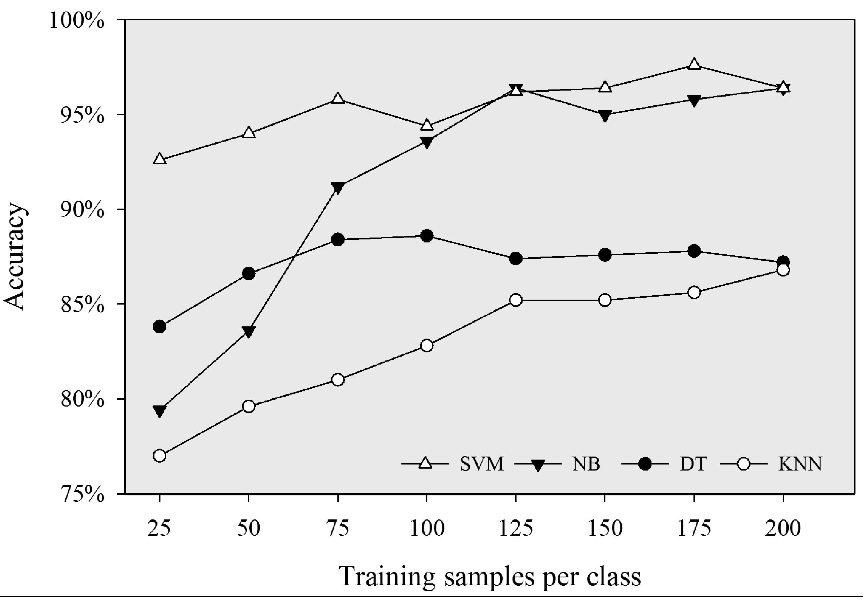
The results showed that SVM generally had the best performance among the four classifiers (
Table 3). With the optimal parameter setting, the minimum overall accuracy and kappa coefficient of SVM was 92.6% and 0.9075, which was higher than the maximum overall accuracy and kappa coefficient of DT (88.4% and 0.855) and KNN (86.8% and 0.835).
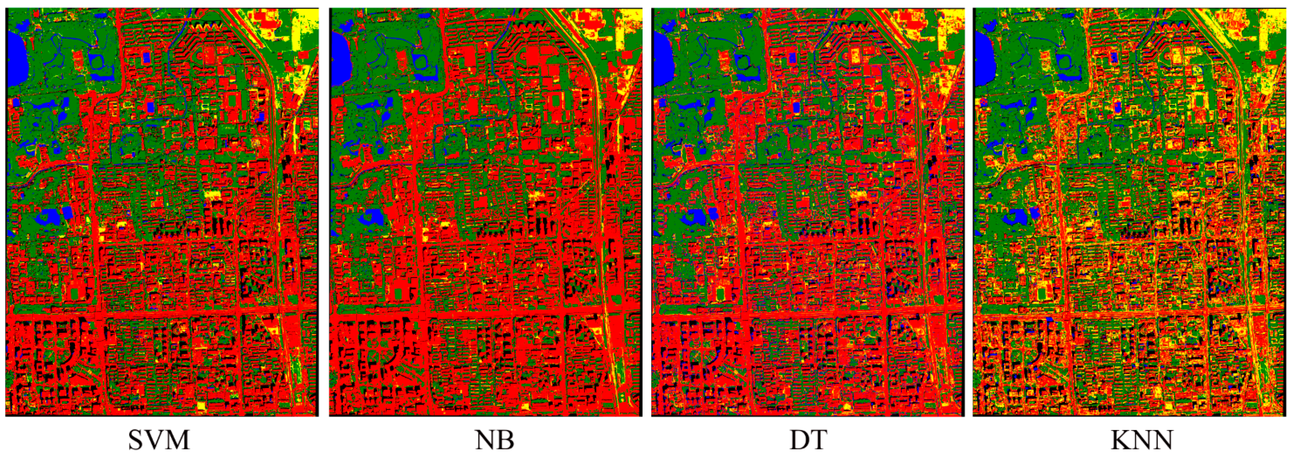
Figure 3 shows the classification results with the highest overall accuracy for each classifier. Using the Z-statistics, we found that the overall accuracies of SVM were significantly greater than those of DT and KNN, regardless of the size of training samples. In addition, SVM had significantly higher overall accuracy than NB, when the size of training samples was relatively small. However, when training samples were greater than or equal to 100 per class, the classification accuracies of NB and SVM were similar and significantly higher than the accuracies of the other two classifiers.
Table 3.
The highest overall accuracy for the four classifiers using eight training sample sets and the corresponding parameter values. NB, normal Bayes; DT, decision tree.
Table 3.
The highest overall accuracy for the four classifiers using eight training sample sets and the corresponding parameter values. NB, normal Bayes; DT, decision tree.
| Sample Size | C | Gamma | Accuracies | Kappa | Sample Size | Max Depth | Accuracies | Kappa |
|---|
| SVM | | | | | DT | | | |
| 25 | 10,000 | 0.001 | 0.926 | 0.9075 | 25 | 3 | 0.838 | 0.7975 |
| 50 | 1,000,000 | 0.00001 | 0.94 | 0.925 | 50 | 5 | 0.866 | 0.8325 |
| 75 | 1,000,000 | 0.00001 | 0.958 | 0.9475 | 75 | 12 | 0.884 | 0.855 |
| 100 | 1,000,000 | 0.00001 | 0.944 | 0.93 | 100 | 6 | 0.884 | 0.855 |
| 125 | 10,000 | 0.0001 | 0.962 | 0.9525 | 125 | 8 | 0.874 | 0.8425 |
| 150 | 10,000 | 0.0001 | 0.964 | 0.955 | 150 | 5 | 0.876 | 0.845 |
| 175 | 1,000,000 | 0.00001 | 0.976 | 0.97 | 175 | 5 | 0.876 | 0.845 |
| 200 | 1,000,000 | 0.00001 | 0.964 | 0.955 | 200 | 6 | 0.872 | 0.84 |
| NB | | | | | KNN | | | |
| 25 | | | 0.794 | 0.7425 | 25 | 1 | 0.77 | 0.7125 |
| 50 | | | 0.836 | 0.795 | 50 | 1 | 0.796 | 0.745 |
| 75 | | | 0.912 | 0.89 | 75 | 3 | 0.81 | 0.7625 |
| 100 | | | 0.936 | 0.92 | 100 | 3 | 0.828 | 0.785 |
| 125 | | | 0.964 | 0.955 | 125 | 1 | 0.852 | 0.815 |
| 150 | | | 0.95 | 0.9375 | 150 | 1 | 0.852 | 0.815 |
| 175 | | | 0.958 | 0.9475 | 175 | 3 | 0.856 | 0.82 |
| 200 | | | 0.964 | 0.955 | 200 | 3 | 0.868 | 0.835 |
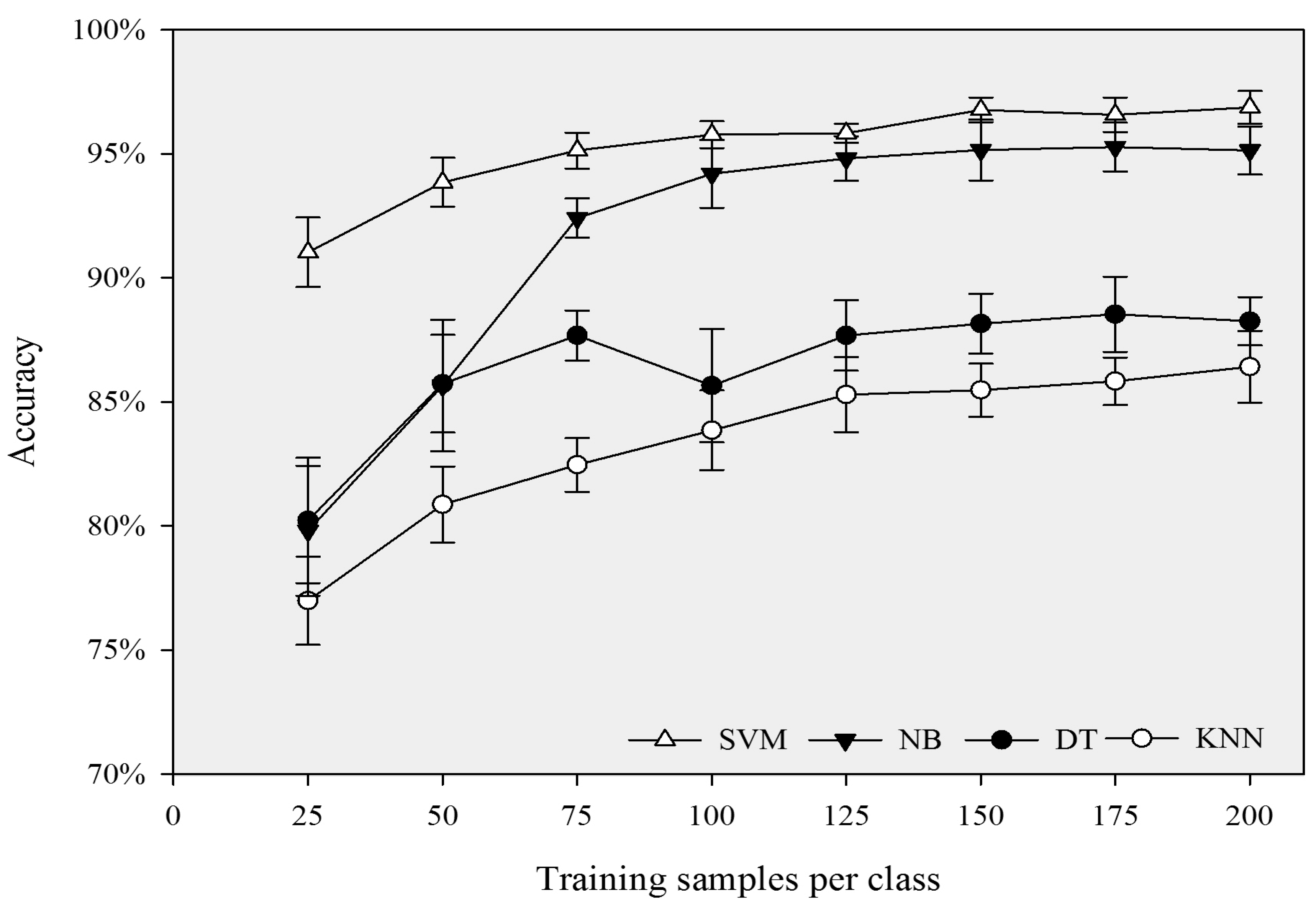
In general, when the size of samples per class was less than 125, the accuracies of the four classifiers increased with increasing size of the training samples, and NB and KNN were more sensitive to sample sizes than SVM and DT. When the size of training samples increased from 25 to 125 per class, the classification accuracies of NB and KNN increased by 17% and 8.2%, while SVM and DT increased by 3.6% and 4.6%, respectively (
Table 3;
Figure 4). NB was the most sensitive to sample size. This may be because this parametric classifier used training samples to estimate parameter values for the data distribution, and thus, more training samples can lead to more accurate parameter estimation. In contrast, SVM is the least sensitive to sample sizes, because SVM only uses the support vectors instead of all training samples to build the separating hyperplane. Thus, adding more training samples may not significantly affect the classification accuracy. However, when the size of the samples is more than 125 per class, all four classifiers become insensitive to the increase of sample sizes. The classification accuracies of NB, KNN, SVM and DT fluctuated from 95% to 96.4%, 85.2% to 86.8%, 96.2% to 97.6% and 87.2% to 87.6%, respectively, with the sample size increasing from 125 to 200 per class. This result indicated that the training sample size of 125 per class might be a turning point, beyond which the increase of sample size does not necessarily lead to a significant increase in classification accuracies. These results have important implications for determining the appropriate sample size.
Figure 3.
The classification results with the highest overall accuracy for each classifier.
Figure 3.
The classification results with the highest overall accuracy for each classifier.
Figure 4.
Overall accuracies of the four classifiers with increasing size of training samples.
Figure 4.
Overall accuracies of the four classifiers with increasing size of training samples.
These findings also have important implications for the selection of appropriate classifiers. In general, SVM is the best candidate classifier for urban land classifications. Using SVM could achieve the best overall classification accuracy, even with a relatively small amount of training samples. However, SVM is sensitive to its tuning parameter setting, which could be subjective and time-consuming. NB can be a practical choice when the training samples are sufficient. NB could achieve similarly high accuracy to that of SVM, but with no need to set any tuning parameter. One of the advantages of using DT is the generation of the “decision tree”, which includes the information of features that are used in classification and the classification rules. This information can be helpful for better understanding the classification process. In addition, in case we want to build a ruleset to conduct a classification, “decision tree” can be a good reference.
4.2. The Effects of Tuning Parameters on Classification Accuracies
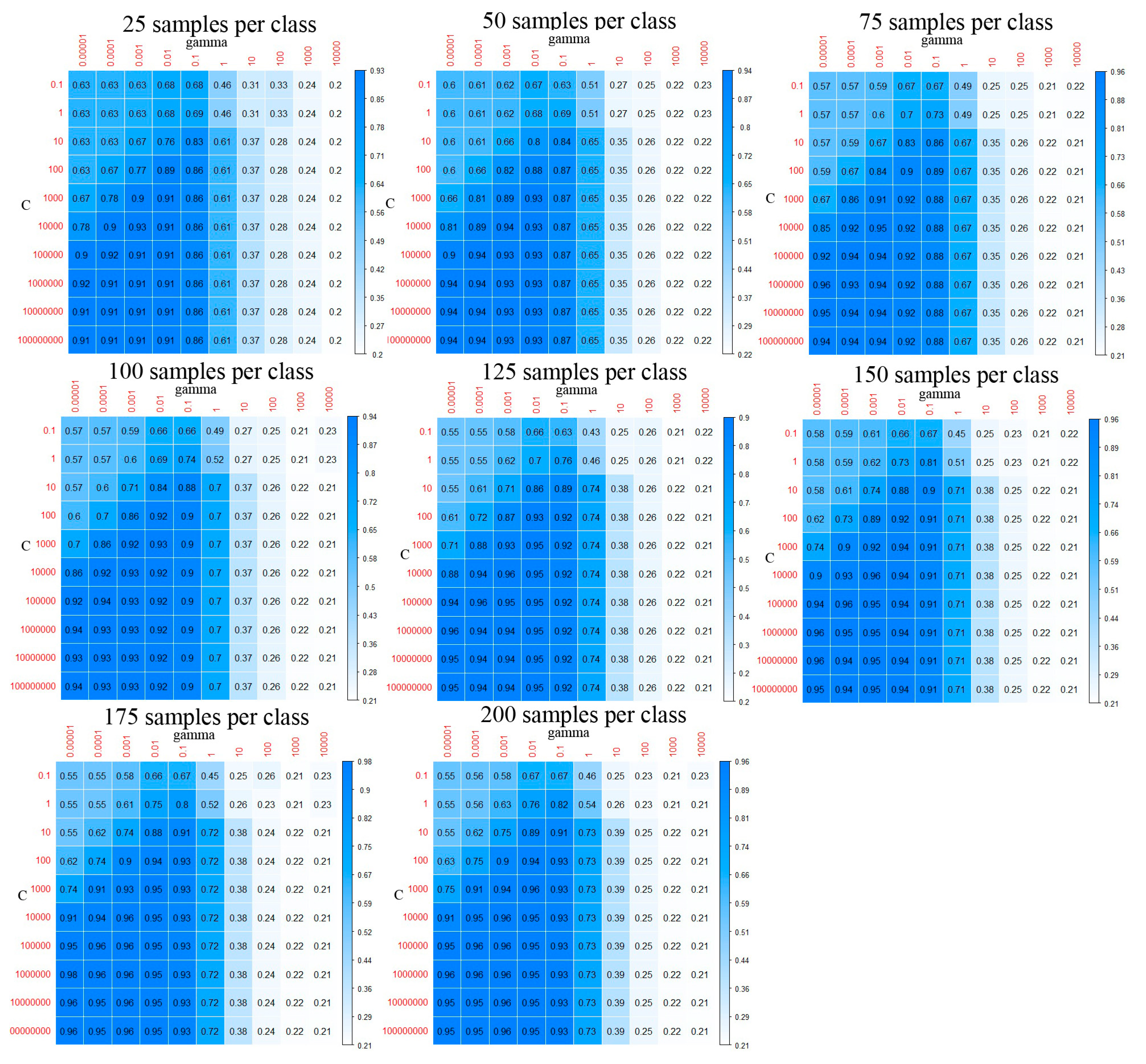
The tuning parameters of the classifier have a great impact on the classification accuracy. We found that SVM was the most sensitive to the setting of tuning parameters, followed by DT. However, KNN was relatively insensitive to the tuning parameter, that is the K. Using the largest training sample set, the classification accuracies of SVM, DT and KNN varied from 21% to 96.4%, 39.4% to 87.2% and 79.4% to 86.8%, respectively, when the settings of tuning parameters were different.
Figure 5.
Matrixes of SVM’s overall accuracies with different values of parameters C and gamma, when using different sizes of training samples. The darker the blue, the higher the accuracy.
Figure 5.
Matrixes of SVM’s overall accuracies with different values of parameters C and gamma, when using different sizes of training samples. The darker the blue, the higher the accuracy.
For SVM, the optimal settings of tuning parameters varied with the sample size. With the training sample sizes of 25, 125 and 150 per class, the optimal values of C and gamma were 10,000 and 0.001, respectively. With the other sample sizes, the optimal values of C and gamma were 1,000,000 and 0.00001, respectively (
Table 3). The matrixes of the classification accuracy (
Figure 5) further provide some insights into how different values of C and gamma, or their combination, affect the classification accuracies of the SVM classifier: (1) when the value of gamma was greater than 0.1, the classification accuracies were relatively low, ranging from 20% to 74%, no matter what value the parameter C was; this result indicated that the value of gamma should not be greater than 0.1; (2) there were ranges of values of C and gamma, at which relatively high accuracies (up to or greater than 90%) could be achieved; in general, these values of C were between 1,000,000 and 100,000,000, and gamma between 0.00001 and 0.001; (3) the sizes of training samples seem not to influence the optimal setting of C and gamma. Very similar patterns were found when using different sizes of training samples. This clearly shows that the effects of tuning parameters on classification accuracy were much greater than that of the size of the training samples.
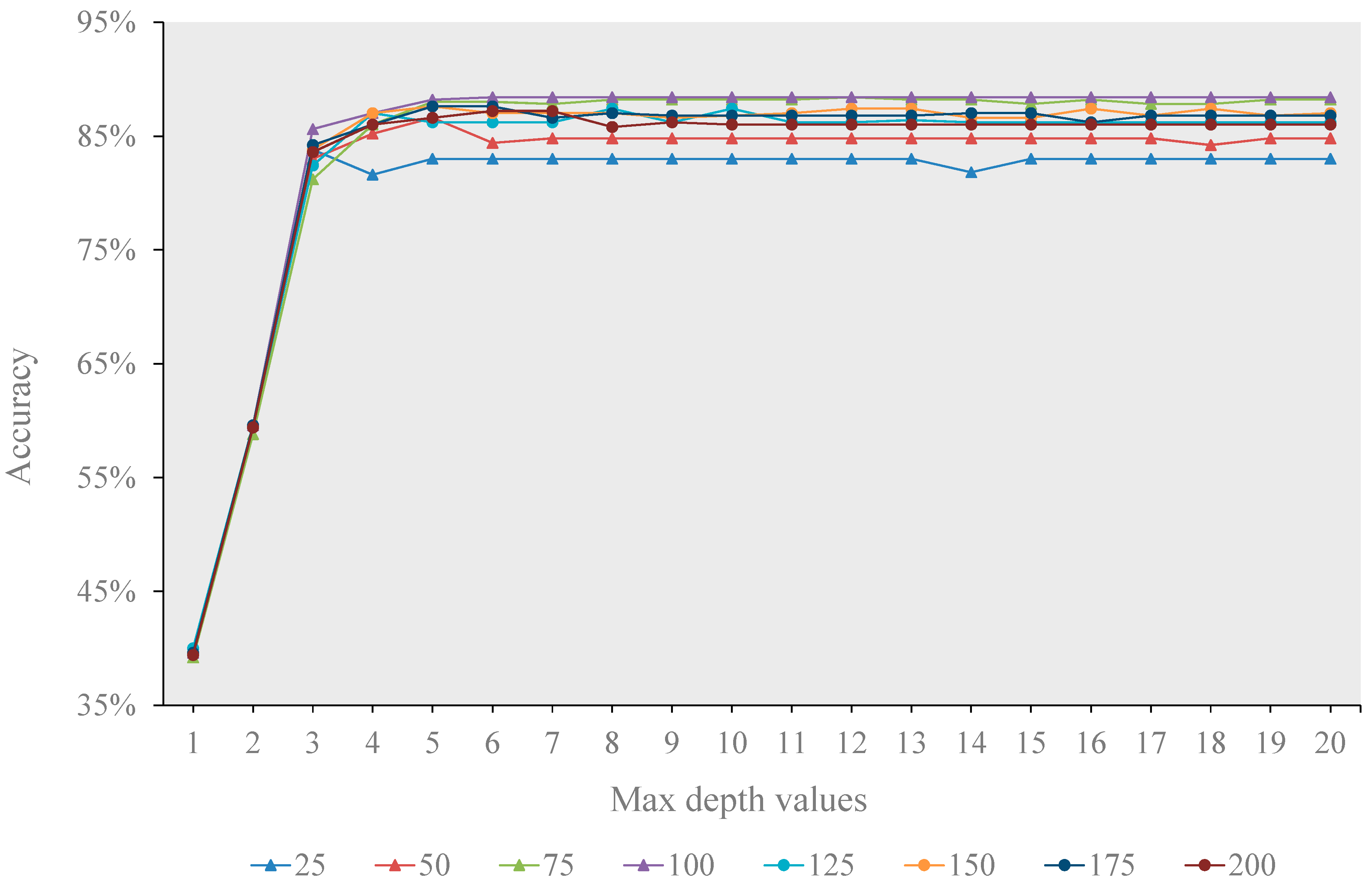
Similarly, for DT, the optimal maximum depth varied greatly with different sizes of training samples (
Figure 6). Generally, the optimal maximum depth mostly fell between five and eight, and the overall classification accuracy became relatively stable when the maximum depth was greater than or equal to five. For KNN, with the increasing of the parameter K, the classification accuracy showed a decreasing fluctuation, regardless of the training sample size (
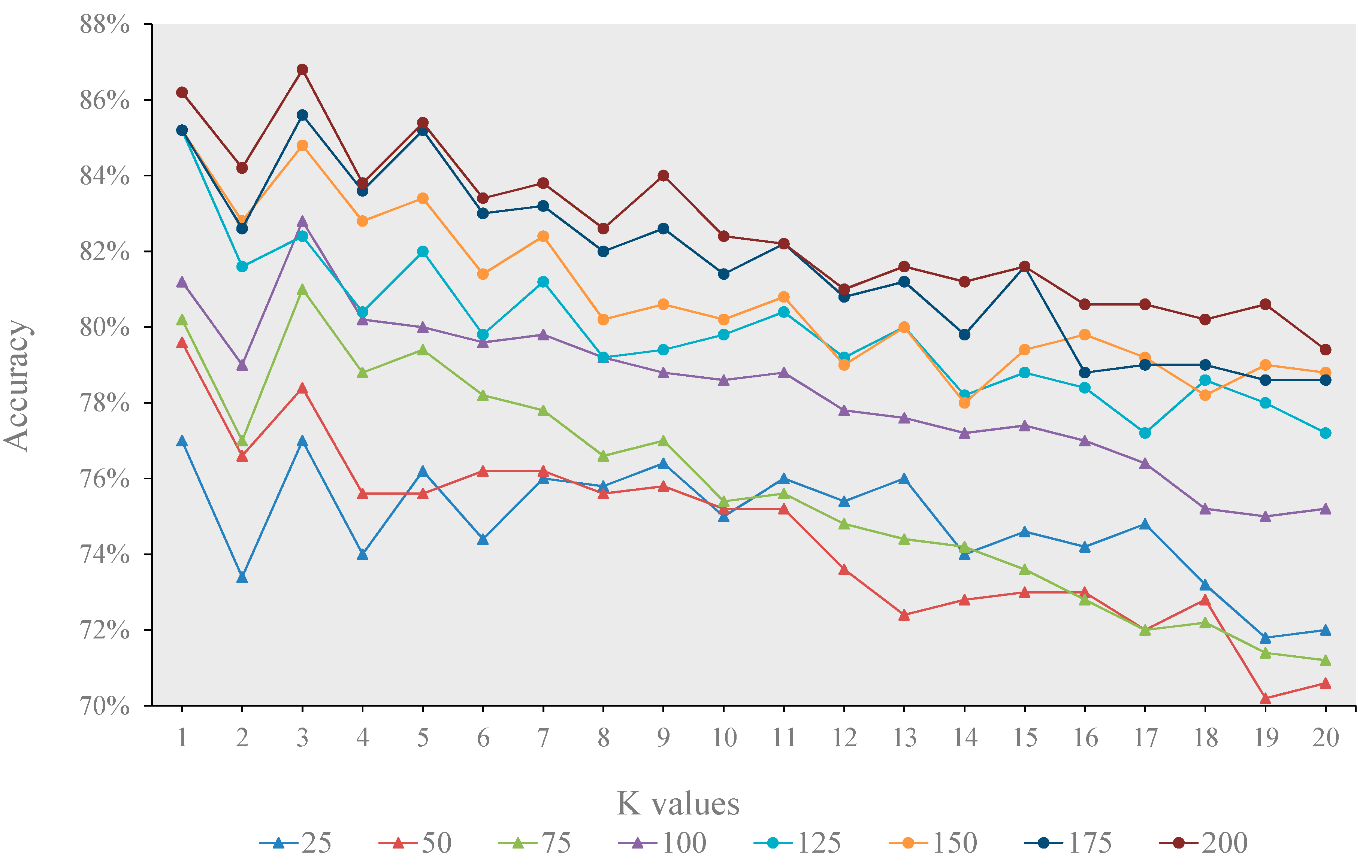
Figure 7). The highest accuracy was often achieved when parameter K was either one or three, suggesting that the performance of KNN is very similar to the nearest neighbor classifier.
Figure 6.
The overall accuracies of DT with the increase of the max depth value.
Figure 6.
The overall accuracies of DT with the increase of the max depth value.
Figure 7.
The overall accuracy of KNN with the increase of the K value.
Figure 7.
The overall accuracy of KNN with the increase of the K value.
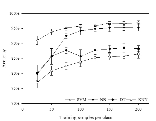
Figure 8.
The average overall accuracies and standard deviation of the four classifiers with optimal parameter settings.
Figure 8.
The average overall accuracies and standard deviation of the four classifiers with optimal parameter settings.
Figure 8 shows the average overall accuracies and the variations of the four classifiers with optimal parameter settings, that is K was three for KNN, the maximum depth was five for DT and C and gamma were 1,000,000 and 0.00001, respectively, for SVM. The changes in average overall accuracies with the sample sizes from the 10-times random sampling were similar to those using the one-time samples (
Figure 4), suggesting that the classifiers were relatively insensitive to the selection of samples. This is particularly true for SVM when the training sample size was greater than 125 per class.
5. Conclusions
In this study, we evaluated and compared the performance of four machine learning classifiers, namely SVM, NB, CART and KNN, in classifying very high resolution images, using an object-based classification procedure. In particular, we investigated how the tuning parameters of each of the classifiers (except for NB) affected the classification accuracy, when using different sizes of training samples. The results showed that SVM and NB were superior to CART and KNN in urban land classification. Both SVM and NB could achieve very high classification accuracy, with appropriate setting of the tuning parameters and/or enough training samples. However, each of the two classifiers has its advantages and disadvantages, and thus, the choice of the appropriate one may be case dependent. SVM could achieve relatively high accuracy with a relatively small amount of training samples, but the setting of tuning parameters could be subjective and time-consuming. In contrast, NB does not need the setting of any tuning parameter, but generally requires a large amount of training samples to achieve relatively high accuracy.
Both the size of training samples and the setting of tuning parameters have great impacts on the performance of classifiers. When the size of training samples is less than 125 per class, increasing the size of training samples generally leads to the increase of classification accuracies for all four classifiers, but NB and KNN were more sensitive to the sample size. Increasing the size of training samples does not seem to significantly improve the classification once the size of training samples reaches 125 per class. The tuning parameters of the classifier had a great impact on the classification accuracy. SVM was the most sensitive to the setting of tuning parameters, followed by DT, but KNN was relatively insensitive to the tuning parameter. While the optimal settings of tuning parameters varied with the size of training samples, some general patterns occurred. For SVM, setting C between 1,000,000 and 100,000,000, and gamma between 0.00001 and 0.001 usually achieved the best overall accuracy. With DT, the best classification accuracy was generally achieved when the max depth of classification tree was between five and eight. For KNN, the optimal K value was either one or three. These findings provide insights into the selection of classifiers and the size of training samples when implementing an object-based approach for urban land classification using high resolution images. This research also highlights the importance of the appropriate setting of tuning parameters for different machine learning classifiers and provides useful information for optimizing those parameters.
Acknowledgments
The support of the National Natural Science Foundation of China (Grant No. 41371197) and the “One hundred talents” program of Chinese Academy of Sciences is gratefully acknowledged. This research was also supported by National Key Technology R&D Program of China during the Twelfth Five-Year Plan Period (2012BAC13B01). Comments from the four anonymous reviewers greatly improved the manuscript.
Author Contributions
Yuguo Qian and Weiqi Zhou designed the research. Yuguo Qian and Weiqi Zhou performed the research. Yuguo Qian and Jingli Yan analyzed the data. Yuguo Qian, Weiqi Zhou, Jingli Yan, Lijian Han and Weifeng Li wrote the paper.
Conflicts of Interest
The authors declare no conflict of interest. The founding sponsors had no role in the design of the study; in the collection, analyses, or interpretation of data; in the writing of the manuscript; nor in the decision to publish the results.
References
- Pu, R.; Landry, S.; Yu, Q. Object-based urban detailed land cover classification with high spatial resolution ikonos imagery. Int. J. Remote Sens. 2011, 32, 3285–3308. [Google Scholar] [CrossRef]
- Malinverni, E.S.; Tassetti, A.N.; Mancini, A.; Zingaretti, P.; Frontoni, E.; Bernardini, A. Hybrid object-based approach for land use/land cover mapping using high spatial resolution imagery. Int. J. Geogr. Infor. Sci. 2011, 25, 1025–1043. [Google Scholar] [CrossRef]
- Zhang, X.; Feng, X.; Jiang, H. Object-oriented method for urban vegetation mapping using ikonos imagery. Int. J. Remote Sens. 2010, 31, 177–196. [Google Scholar]
- Myint, S.W.; Gober, P.; Brazel, A.; Grossman-Clarke, S.; Weng, Q. Per-pixel vs. object-based classification of urban land cover extraction using high spatial resolution imagery. Remote Sens. Environ. 2011, 115, 1145–1161. [Google Scholar]
- Duro, D.C.; Franklin, S.E.; Dube, M.G. A comparison of pixel-based and object-based image analysis with selected machine learning algorithms for the classification of agricultural landscapes using SPOT-5 HRG imagery. Remote Sens. Environ. 2012, 118, 259–272. [Google Scholar] [CrossRef]
- Blaschke, T. Object based image analysis for remote sensing. ISPRS J. Photogramm. Remote Sens. 2010, 65, 2–16. [Google Scholar] [CrossRef]
- Zhou, W.; Cadenasso, M.L.; Schwarz, K.; Pickett, S.T. Quantifying spatial heterogeneity in urban landscapes: Integrating visual interpretation and object-based classification. Remote Sens. 2014, 6, 3369–3386. [Google Scholar] [CrossRef]
- Zhou, W.; Troy, A. An object-oriented approach for analysing and characterizing urban landscape at the parcel level. Int. J. Remote Sens. 2008, 29, 3119–3135. [Google Scholar] [CrossRef]
- Laliberte, A.S.; Koppa, J.; Fredrickson, E.L.; Rango, A. Comparison of nearest neighbor and rule-based decision tree classification in an object-oriented environment. In Proceedings of the IEEE International Geoscience and Remote Sensing, Denver, CO, USA, 31 July–4 August 2006.
- Laliberte, A.S.; Rango, A.; Havstad, K.M.; Paris, J.F.; Beck, R.F.; McNeely, R.; Gonzalez, A.L. Object-oriented image analysis for mapping shrub encroachment from 1937 to 2003 in Southern New Mexico. Remote Sens. Environ. 2004, 93, 198–210. [Google Scholar] [CrossRef]
- Pal, M. Random forest classifier for remote sensing classification. Int. J. Remote Sens. 2005, 26, 217–222. [Google Scholar] [CrossRef]
- McInerney, D.O.; Nieuwenhuis, M. A comparative analysis of kNN and decision tree methods for the irish national forest inventory. Int. J. Remote Sens. 2009, 30, 4937–4955. [Google Scholar] [CrossRef]
- Song, X.; Duan, Z.; Jiang, X. Comparison of artificial neural networks and support vector machine classifiers for land cover classification in northern China using a SPOT-5 HRG image. Int. J. Remote Sens. 2012, 33, 3301–3320. [Google Scholar] [CrossRef]
- Huang, C.; Davis, L.S.; Townshend, J.R.G. An assessment of support vector machines for land cover classification. Int. J. Remote Sens. 2002, 23, 725–749. [Google Scholar] [CrossRef]
- Buddhiraju, K.M.; Rizvi, I.A. Comparison of CBF, ANN and SVM classifiers for object based classification of high resolution satellite images. In Proceedings of the 2010 IEEE International Geoscience and Remote Sensing Symposium (IGARSS), Honolulu, HI, USA, 25–30 July 2010; pp. 40–43.
- Wieland, M.; Pittore, M. Performance evaluation of machine learning algorithms for urban pattern recognition from multi-spectral satellite images. Remote Sens. 2014, 6, 2912–2939. [Google Scholar] [CrossRef]
- Shiraishi, T.; Motohka, T.; Thapa, R.B.; Watanabe, M.; Shimada, M. Comparative assessment of supervised classifiers for land use–land cover classification in a tropical region using time-series palsar mosaic data. IEEE J. Sel. Top. Appl. Earth Obs. Remote Sens. 2014, 7, 1186–1199. [Google Scholar] [CrossRef]
- Vanniel, T.; McVicar, T.; Datt, B. On the relationship between training sample size and data dimensionality: Monte carlo analysis of broadband multi-temporal classification. Remote Sens. Environ. 2005, 98, 468–480. [Google Scholar] [CrossRef]
- Foody, G.M.; Mathur, A.; Sanchez-Hernandez, C.; Boyd, D.S. Training set size requirements for the classification of a specific class. Remote Sens. Environ. 2006, 104, 1–14. [Google Scholar] [CrossRef]
- Yan, G.; Mas, J.F.; Maathuis, B.H.P.; Xiangmin, Z.; van Dijk, P.M. Comparison of pixel-based and object-oriented image classification approaches—A case study in a coal fire area, Wuda, Inner Mongolia, China. Int. J. Remote Sens. 2006, 27, 4039–4055. [Google Scholar] [CrossRef]
- Zhou, W.; Troy, A. Development of an object-based framework for classifying and inventorying human-dominated forest ecosystems. Int. J. Remote Sens. 2009, 30, 6343–6360. [Google Scholar] [CrossRef]
- Trimble. In Ecognition Developer 8.7 Reference Book; Trimble: Munich, Germany, 2011.
- Bradski, G.; Kaehler, A. Learning Opencv: Computer Vision with the Opencv Library; O’Reilly Media, Inc.: Sebastopol, CA, USA, 2008. [Google Scholar]
- Breiman, L.; Friedman, J.H.; Olshen, R.A.; Stone, C.J. Classification and Regression Trees; Wadsworth & Brooks: Monterey, CA, USA, 1984. [Google Scholar]
- Vapnik, V.; Chervonenkis, A. On the uniform convergence of relative frequencies of events to their probabilities. Theory Probab. Appl. 1971, 16, 264–280. [Google Scholar] [CrossRef]
- Kavzoglu, T.; Colkesen, I. A kernel functions analysis for support vector machines for land cover classification. Int. J. Appl. Earth Obs. Geoinf. 2009, 11, 352–359. [Google Scholar]
- Burges, C.J. A tutorial on support vector machines for pattern recognition. Data Min. Knowl. Discov. 1998, 2, 121–167. [Google Scholar] [CrossRef]
- Lin, S.-L.; Liu, Z. Parameter selection in SVM with RBF kernel function. J. Zhejiang Univ. Technol. 2007, 35, 163. [Google Scholar]
- Zhang, H. The Optimality of Naive Bayes. Available online: http://www.cs.unb.ca/profs/hzhang/publications/FLAIRS04ZhangH.pdf (accessed on 17 December 2014).
- Erener, A. Classification method, spectral diversity, band combination and accuracy assessment evaluation for urban feature detection. Int. J. Appl. Earth Obs. Geoinf. 2013, 21, 397–408. [Google Scholar] [CrossRef]
© 2014 by the authors; licensee MDPI, Basel, Switzerland. This article is an open access article distributed under the terms and conditions of the Creative Commons Attribution license (http://creativecommons.org/licenses/by/4.0/).


