Mapping Layers of Clay in a Vertical Geological Surface Using Hyperspectral Imagery: Variability in Parameters of SWIR Absorption Features under Different Conditions of Illumination

Abstract
: Hyperspectral imagery of a vertical mine face acquired from a field-based platform is used to evaluate the effects of different conditions of illumination on absorption feature parameters wavelength position, depth and width. Imagery was acquired at different times of the day under direct solar illumination and under diffuse illumination imposed by cloud cover. Imagery acquired under direct solar illumination did not show large amounts of variability in any absorption feature parameter; however, imagery acquired under cloud caused changes in absorption feature parameters. These included the introduction of a spurious absorption feature at wavelengths > 2250 nm and a shifting of the wavelength position of specific clay absorption features to longer or shorter wavelengths. Absorption feature depth increased. The spatial patterns of clay absorption in imagery acquired under similar conditions of direct illumination were preserved but not in imagery acquired under cloud. Kaolinite, ferruginous smectite and nontronite were identified and mapped on the mine face. Results were validated by comparing them with predictions from x-ray diffraction and laboratory hyperspectral imagery of samples acquired from the mine face. These results have implications for the collection of hyperspectral data from field-based platforms.
1. Introduction
Identifying and mapping clay minerals on vertical outcrops of geology or on mine faces in open-pit mines is important for economic reasons and safety. Thin layers of clay shales (2–30 cm thick) are often used by geologists as marker horizons to delineate geological units of similar appearance [1,2]. On mine faces, the relative positions of clay layers in the stratigraphic sequence are used to guide the extraction of ore from the mine face and as indicators for separating zones of ore from waste. In the context of remote sensing, the position of clay layers within the stratigraphy could potentially be used as a basis for the contextual classification of geological units in cases where they could not be distinguished on the basis of their spectral signature alone. Layers of clay also represent planes of stratigraphical weakness along which major landslides can occur [3,4]. Even relatively thin layers of clay can potentially increase the risk of slippage [5]. For example, 2–6 cm thick layers of clay in coal seams—so called clay mylonites—represent planes of weakness which can significantly increase the risk of slippage or failure along their length [6,7]. Clays, by attracting water into their layered structure, can undergo an expansion of up to four times their volume when transitioning from a dry to a saturated state [8]. Smectite-group clays have the greatest potential to swell and therefore present the greatest capacity for failure because they undergo repeated successive phases of expansion and contraction, causing localized disturbance and ground heave [8–11]. Identifying the types and abundance of clay minerals in these layers provides information that can be incorporated into assessments of risks or models of potential slope failure in road cuttings or in open pit mines, e.g., [12]. Mapping of clay layers in the field by visual inspection is problematic because it is labor-intensive and dangerous. It is also difficult, even for experienced geologists, to determine the types of clay present in the layers.
Hyperspectral imagery (SWIR; 2000–2450 nm) acquired from field-based platforms has the potential to provide the high (cm-scale) spatial resolutions required to map clays. Several analytical techniques such as the spectral angle mapper, SAM [13], the USGS tetracorder [14] or spectral unmixing, e.g., [15,16], have been used to map clay minerals by exploiting differences in their spectral curve shape caused by the presence or absence of diagnostic absorption features. Although these techniques can tell us something about the spatial distribution of clays, e.g., [17], they do not provide any information per se about their physical or chemical composition nor can they be applied to data without the use of a spectral library. Alternatively, clays can be detected or mapped by parameterising their diagnostic absorption features in the SWIR [18,19]. These features occur as a result of the hydroxyl (OH) stretch and metal-OH bend [20,21]. The parameters of absorption features include wavelength position, width and depth and these can be used directly to map clay minerals, e.g., [18,22], or as inputs to expert systems, e.g., [23]. Wavelength position, in particular, provides information related to the type of cation involved with Al, Mg, or Fe causing OH absorptions near 2210 nm, 2290 nm and 2320 nm, respectively [24]. Smaller shifts in the wavelength position of features close to 2200 nm have been related to the abundance of Al in octahedral sites in the crystal lattice of some phyllosilicates [25]. The depth of absorption features is related to abundance or the grain size of the absorbing mineral [26]. Absorption feature parameters are therefore intrinsically linked to the physical processes causing absorption and, as such, provide important information about the chemical composition of minerals. For these reasons, feature parameterization provides a powerful tool to extract information about clay mineralogy from spectra. Furthermore, this approach requires no spectral library, enabling clay minerals to be mapped without a priori knowledge of any particular surface.
To date, most studies have used hyperspectral images collected from airborne platforms, i.e., from an overhead or nadir perspective [27]. Because airborne data are expensive to collect, repeated flights over the same target are rarely done. Consequently, there is little or no information about if or how changing conditions of illumination (e.g., variable solar angles or cloud cover) might affect feature parameters derived from imagery acquired from field-based platforms. The first objective of this paper is therefore to quantify any changes in absorption feature parameters which might occur in imagery from the same target in response to different conditions of illumination caused by variable sun-angles or cloud cover (Experiment 1). The target surface used in this study is a vertical mine wall in an open-pit iron-ore mine in the Pilbara, Western Australia. If maps derived from feature parameters of the same surface were not comparable when viewed under different conditions of illumination, this would limit their usefulness. The map would change according to illumination—a factor which is unrelated to mineralogy. Such effects would, at the very least, constrain the conditions under which the imagery could be collected. The second objective of this paper therefore is to determine if, and to what degree, changing conditions of illumination during the course of the day might change maps of clay minerals derived from absorption feature parameters (Experiment 2). The third and final objective of this paper is to use hyperspectral imagery to map and quantify clay mineralogy on a mine wall (Experiment 3). Clay minerals are often distributed in discrete layers sometimes only a few cm thick. Delineation of these thin layers would enable mining companies to unambiguously assign geological boundaries to areas of the mine face and/or to determine the potential lines along which any slippage might occur. In this experiment we use imagery acquired under “optimal” conditions where the mine face is illuminated by direct sunlight.
2. Materials and Methods
2.1. Study Area
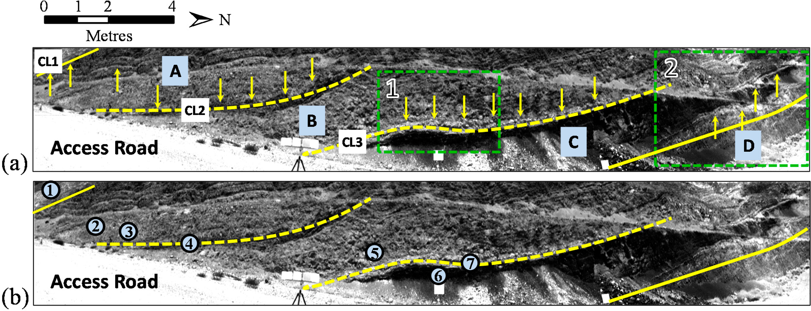
The study area was located in an iron ore mine in the Pilbara, Western Australia (24°12′52.77″S; 114°50′23.33″E). The rocks in this area are characterized by late Archaean and early Proterozoic rocks including Banded Iron Formation (BIF), Whaleback shale and black shale [1,28]. BIF is composed of alternating bands of magnetite and hematite which has, in places, become mineralized by removal of silica through hypogene and supergene processes. Whaleback shale is a thick sedimentary unit containing hematite, goethite, maghemite and silica but, generally, contains little clay. Black shale, rich in vermiculite, is also present. Thin layers of volcanic or sedimentary clay are dispersed within and between these major rock units (Figure 1; Table 1).
2.2. Hyperspectral Imagery
Hyperspectral imagery was acquired using a SWIR (1000–2500 nm) imaging sensor (Specim, Finland). The sensor was configured to have a nominal full-width-half-maximum (FWHM) bandwidth of 6 nm. According to the manufacturer, smile and keystone effects were quantified as less than 20% of the pixel size, so correction for these effects was not required. All data were corrected for contribution of dark current in each band by subtracting the dark current signal on a line-by-line basis.
2.2.1. Field Imagery
To protect against high ambient temperatures (>50 ºC) and airborne dust the sensor was enclosed in an environmentally-controlled box. Cooled, filtered, desiccated air was pumped into the top of the box and exhausted through the bottom. The sensor and enclosure were mounted on a rotating stage attached to the top of a tripod. The distance from the sensors to the mine face was 10 m, thus yielding a spatial pixel size of 0.46 cm × 0.46 cm.
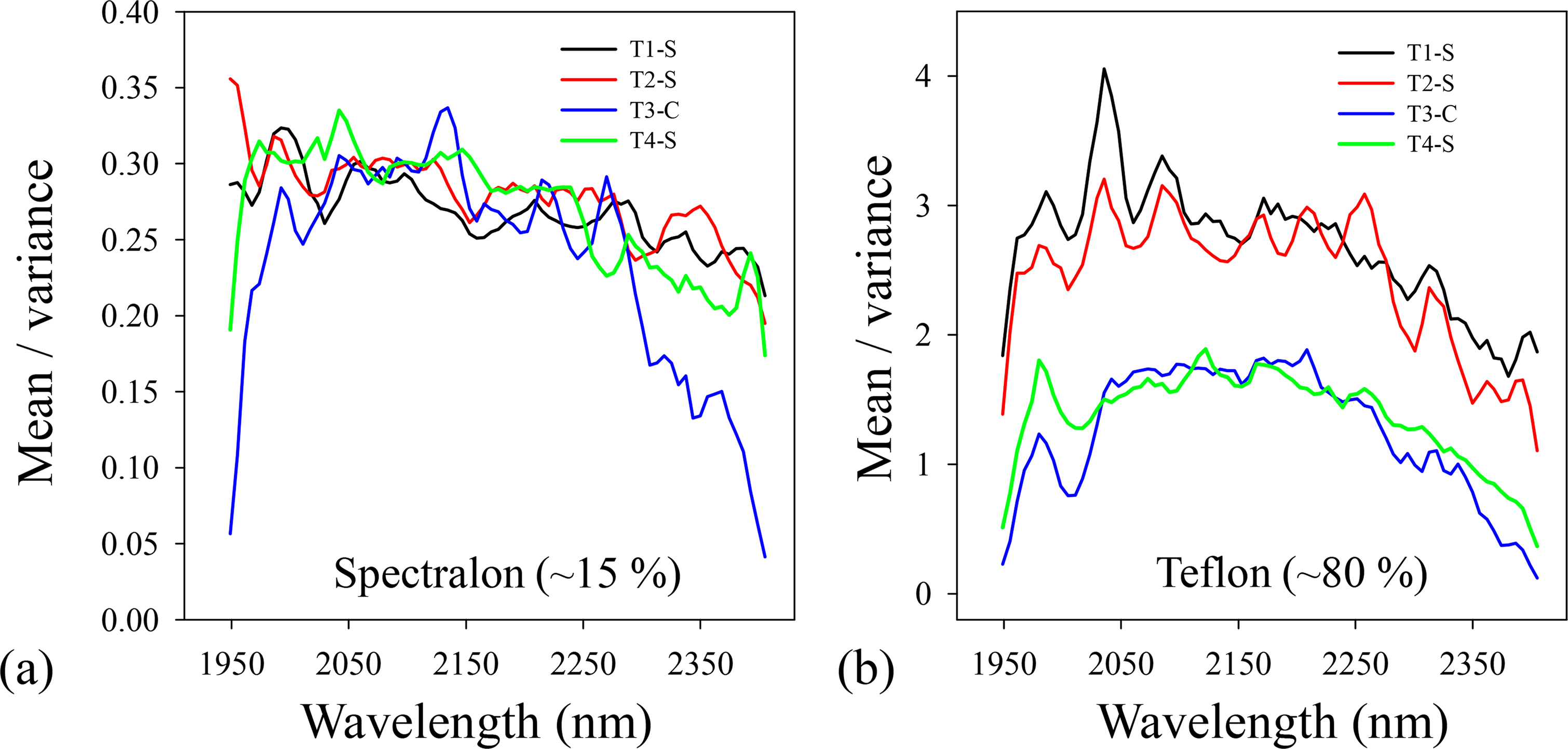
Several calibration panels of different brightness were placed in the field of view of the imager. These comprised 15%, 30% and 99% reflective Spectralon® and ∼80% reflective Teflon. All panels were placed at the same angle of orientation as the mine face. The integration time of the sensor was set according to the ambient conditions of illumination so that pixels over the calibration panels were not saturated. Numerous images were acquired under variable conditions of solar illumination; however, four images were selected for use in this study (Table 2). The first image (T1-S) was acquired under “optimal” conditions with the sun fully and directly illuminating the mine face; the second image (T2-S) was acquired shortly after T1-S, under similar conditions of illumination and sun-angle, thus effectively replicating the conditions under which T1-S was acquired; the third image (T3-C) was acquired under stable illumination but under low-altitude cloud allowing the mine face to be illuminated with diffuse light; the fourth image (T4-S) was acquired under direct sunlight which illuminated the mine face at a more acute angle, causing parts of the mine face to become shaded by overhanging rocks.
All images were calibrated to absolute reflectance using the same calibration target (∼80% Teflon), on a band-by-band basis, using the flat field method. For each image band, pixel values in the image were divided by the average of the pixel values over the calibration panel and the result multiplied by the calibration factor of the Teflon panel. Image spectra were smoothed using an 9-band smoothing window using the method of Savitzky and Golay [29] with a polynomial of the second degree. This removed high-frequency noise whilst preserving the shape of the spectral curve and the wavelength position of absorption features. It is acknowledged that any smoothing filter has the capacity to shift the wavelength position of absorption maxima, however this was not apparent in these data.
2.2.2. Laboratory imagery
The SWIR imager was mounted on a metal scanning frame to obtain images from rock samples acquired in the field (see Section 2.3). Samples were placed on a moving scanning tray beneath the sensor, at a nominal distance of 730 mm. The source of illumination was two arrays of seven halogen lights. A calibration measurement was taken by placing a calibration panel (∼80% Teflon) within the field of view of the sensor. About 500 frames of data were acquired without moving the scanning tray. Imagery was then acquired from the rock samples. The integration time of the sensor was set so that the data occupied the full dynamic range of the data (16-bits), without saturating any pixels.
To remove spatial variations in illumination incident upon the rock samples, calibration to absolute reflectance was done separately for each spatial line recorded by the sensor. This was done for each band by dividing each spatial line in the target (i.e., sample) image by the average value of the corresponding line in the calibration image. The result was then multiplied by the reflectance factor of the calibration panel.
2.3. Rock Samples and X-Ray Diffraction (XRD) Analysis
Sampling of rocks on the mine face was constrained by considerations for safety and was limited to the lower part of the mine face, within easy reach of the road. Rock samples were collected from the major geological units identified in the field (Figure 1A–D; Table 2) and from the 2 major layers of clay which separated units A and B and units B and C (Figure 1; Table 2). Between 2 and 5 representative rock samples were collected within a 50 × 50 cm plot at each of these locations. The reason for sampling the geological units between the observed layers of clay was to determine if they were compositionally different to the layers of clay which separated them.
Minerals were then identified from each sample using quantitative X-Ray Diffraction (XRD) analysis. Samples were ring-milled with an internal standard and micronized. XRD patterns were measured using a Bruker-AXS D8 Advance Diffractometer with cobalt radiation. Crystalline phases were identified by using a search/match algorithm (DIFFRAC.EVA 2.1; Bruker-AXS, Germany). Relevant crystal structures extracted for refinement were obtained from the Inorganic Crystal Structure Database (ICSD 2012/1). The crystalline phases were determined on an absolute scale using Rietveld quantitative phase refinement, using the Bruker-AXS TOPAS v4.2 software package.
2.4. Analyses of Imagery
2.4.1. Determining Relative Amounts of Noise in Imagery
To determine the relative amounts of noise across all images, a rectangular block of 120 pixels were extracted from the center of a homogenous dark target (15% reflective Spectralon panel) and a homogenous bright target (∼80% reflective Teflon panel). For each band, the means and variances of these pixels were calculated. Amounts of noise for each band and target were calculated as the mean divided by the variance (Figure 2; Table 3). It should be noted that the derived values are only intended to be used as a measure of the relative amounts of noise between images and not an absolute measure of the signal-to-noise ratio.
2.4.2. Automated Feature Extraction (AFE)
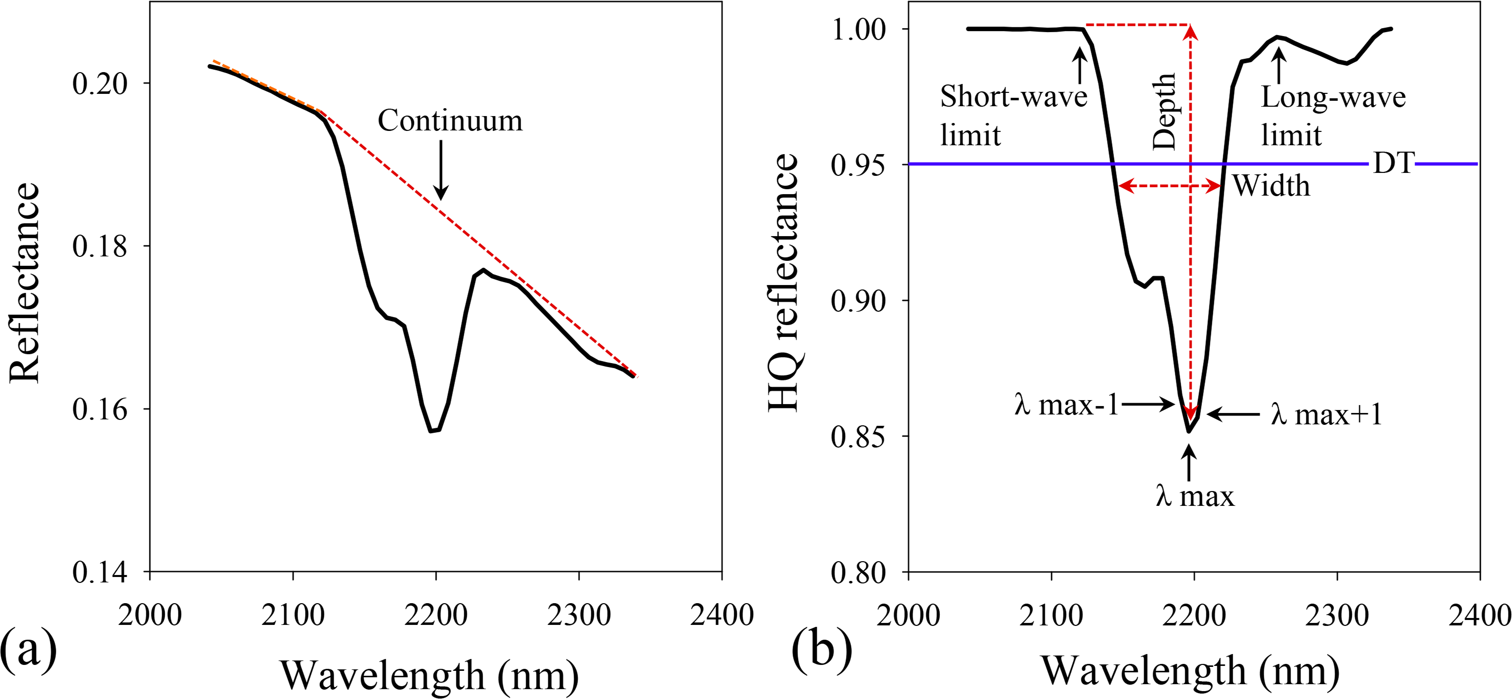
The spectral continuum was removed using a hull-quotients procedure, i.e., dividing the reflectance at each pixel in the image by its upper convex hull [30]. The wavelength position, depth and width of the strongest (i.e., the deepest) absorption feature in each pixel spectrum was determined by AFE (Figure 3). Due to noise in the spectrum (Figure 2), the removal of the spectral continuum was constrained to wavelengths between 2041 and 2337 nm. The deepest absorption feature was identified as the smallest hull-quotients value in each pixel spectrum. However, as a consequence of noise, hull-quotients spectra without any observable absorption features often had minimal values that fell within the range 0.95 to 0.99. Preliminary tests indicated that true absorption features with a hull-quotients value of greater than 0.95 could not be distinguished from noise. A “depth threshold” of 0.95 was therefore set so that only features which had hull-quotients minima equal to or smaller than this value were considered to be “coherent” absorptions for subsequent parameterization by AFE. Pixels which had hull-quotient minima which were greater than the depth threshold were set to zero. AFE was applied to the same imagery with and without the depth threshold being set. This resulted in two AFE analyses for each of the 4 replicate images. Depth was determined in accordance with [30]. Wavelength position of the deepest feature was determined by the quadratic method of Rodger et al. [31]. For each AFE analysis, separate “parameter images” were created describing the wavelength position, depth and width of the deepest absorption feature in each pixel spectrum.
2.4.3. Experiment 1—Variation of Absorption Feature Parameters across Images
Absorption feature parameters across replicate images were compared in two separate analyses. First, to identify any general patterns of change in absorption feature parameters across images, the frequency of pixels describing wavelength position, depth and width within a spatial subset (Subset 1; Figure 1a) of each image were calculated and compared. The use of a spatial subset containing a prominent clay layer ensured that a larger proportion of pixels would contain absorption features than would have been the case if data from the entire image had been used. Second, changes in the parameters of absorption features located at specific wavelengths were determined between image T1-S and, respectively, T2-S, T3-C and T4-S. T1-S was selected as the “baseline” image because it was acquired under “optimal” conditions of illumination. It had, on average, the smallest amount of noise of any image, including T2-S, and which was acquired under similar conditions (Tables 1 and 3; Figure 2, bright target). Thus, absorption feature parameters derived from all other images were compared directly, pixel by pixel, with those from imagery acquired under “optimal” conditions. To do this, we focused specifically on pixels with absorption features with wavelengths at 2196 nm and 2202 nm (kaolinite) and 2288 nm (nontronite) as identified by the AFE wavelength parameter image of T1-S. Kaolinite is unambiguously identified by an absorption doublet centered on 2200 nm and a second, less intense absorption at 2160 nm [20]. Image spectra with absorption maxima centered on 2196 and 2202 nm both exhibited these spectral features and were therefore considered to be kaolinite. The same pixels were then identified in T2-S, T3-C and T4-S. To determine if absorption feature parameters in these images changed in relation to T1-S, images of each feature parameter derived from image T1-S were subtracted from the corresponding feature parameter derived from images T2-S, T3-C and T4-S.
2.4.4. Experiment 2—Spatial Patterns of Clay Absorption across Images
Spatial patterns in clay absorption were examined using the absorption feature parameters wavelength position, depth and width from image Subset 1 (see Figure 1a for context). This subset was chosen because it corresponded to the area used to examine changes in absorption feature parameters and because it presented well-defined clay layers of different composition. Patterns of clay absorption across each image were assessed qualitatively. A quantitative assessment was made using the number of absorption features which were found by AFE in each image. It was expected that, with increasing amounts of noise, there would be an increase in the number of spurious features found by AFE and, thus, a corresponding increase in high-frequency spatial noise in the parameter images.
2.4.5. Experiment 3—Delineation and Quantification of Clay Layers across the Entire Mine Face
Image T1-S, with the least amount of noise over the brightest calibration panel was selected to map clay layers on the mine face. AFE was used with a depth threshold of 0.95 to determine the wavelength position of the deepest absorption feature in each pixel spectrum (indicative of mineral type) and its depth (indicative of mineral abundance). The width parameter did not provide additional information on the clay minerals present and was not used.
XRD data from the rock samples were used to predict which plots would contain absorption features associated with clay minerals. Separately, for each sample plot, average spectra of the rock samples (from laboratory imagery) were compared with average spectra from field imagery of the mine face.
3. Results
3.1. Experiment 1—Variation of Absorption Feature Parameters across Images
3.1.1. General Patterns of Change of Absorption Feature Parameters
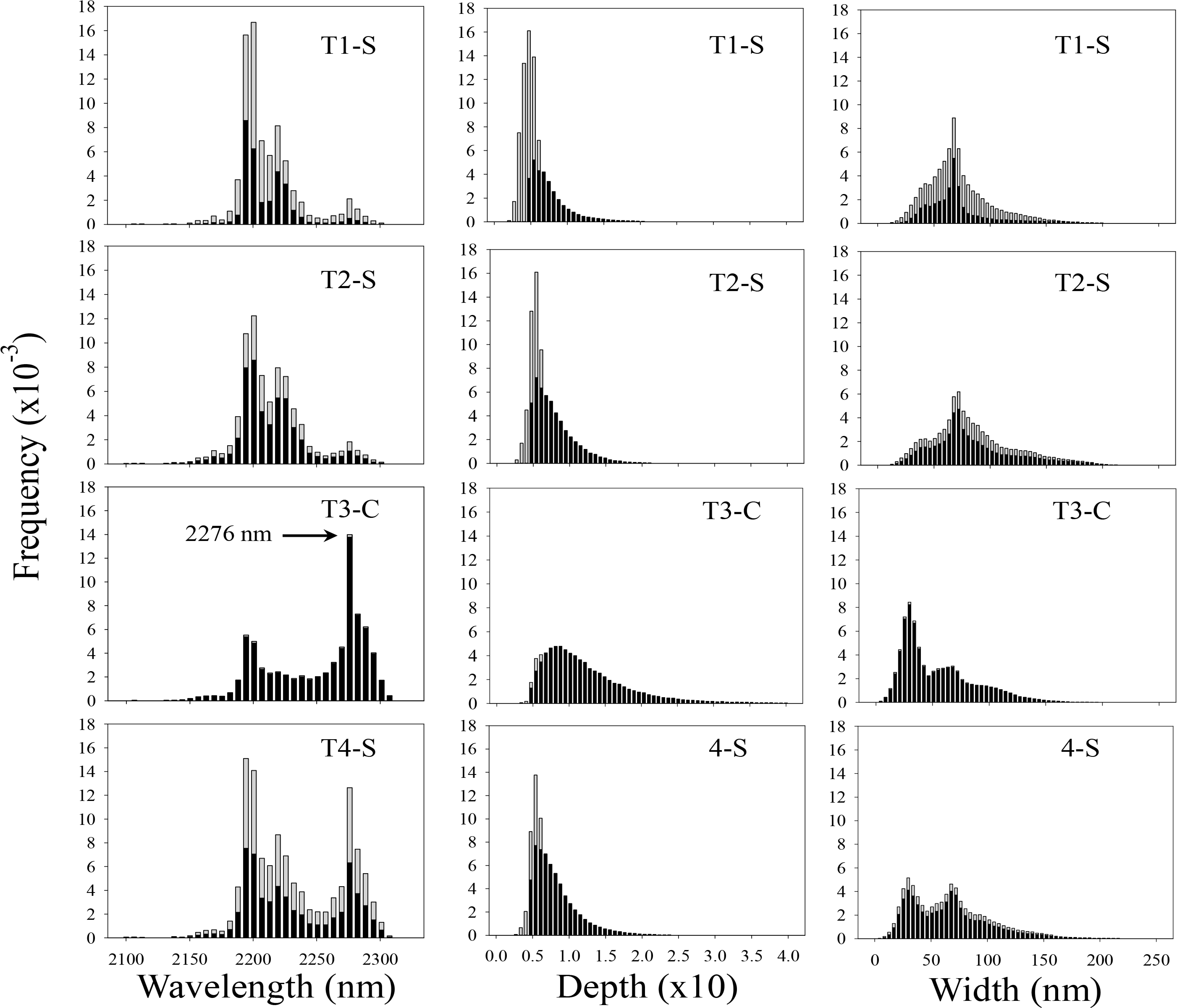
The frequency distribution of pixel values for each feature attribute and each image showed that there were large amounts of variability in parameters among images (Figure 4). The distribution of pixel values representing wavelength position for T1-S and T2-S were very similar; this was expected because these images were acquired under similar conditions of illumination. T1-S, T2-S and T4-S had large numbers of pixels which were excluded by the depth threshold (as indicated by the relatively large differences in number of pixels represented by the grey and black bars). Images T3-C and T4-S had a much larger number of pixels with an absorption feature at wavelengths greater than 2250 nm, however, the distribution of pixels with an absorption feature at wavelengths of less than 2250 nm in T4-S were similar to those found for T1-S and T2-S. Image T3-C was different to all other images because nearly all pixels in the image were included by the depth threshold, i.e., they were considered by AFE to have absorption features, as indicated by the dominance of black bars in the graph.
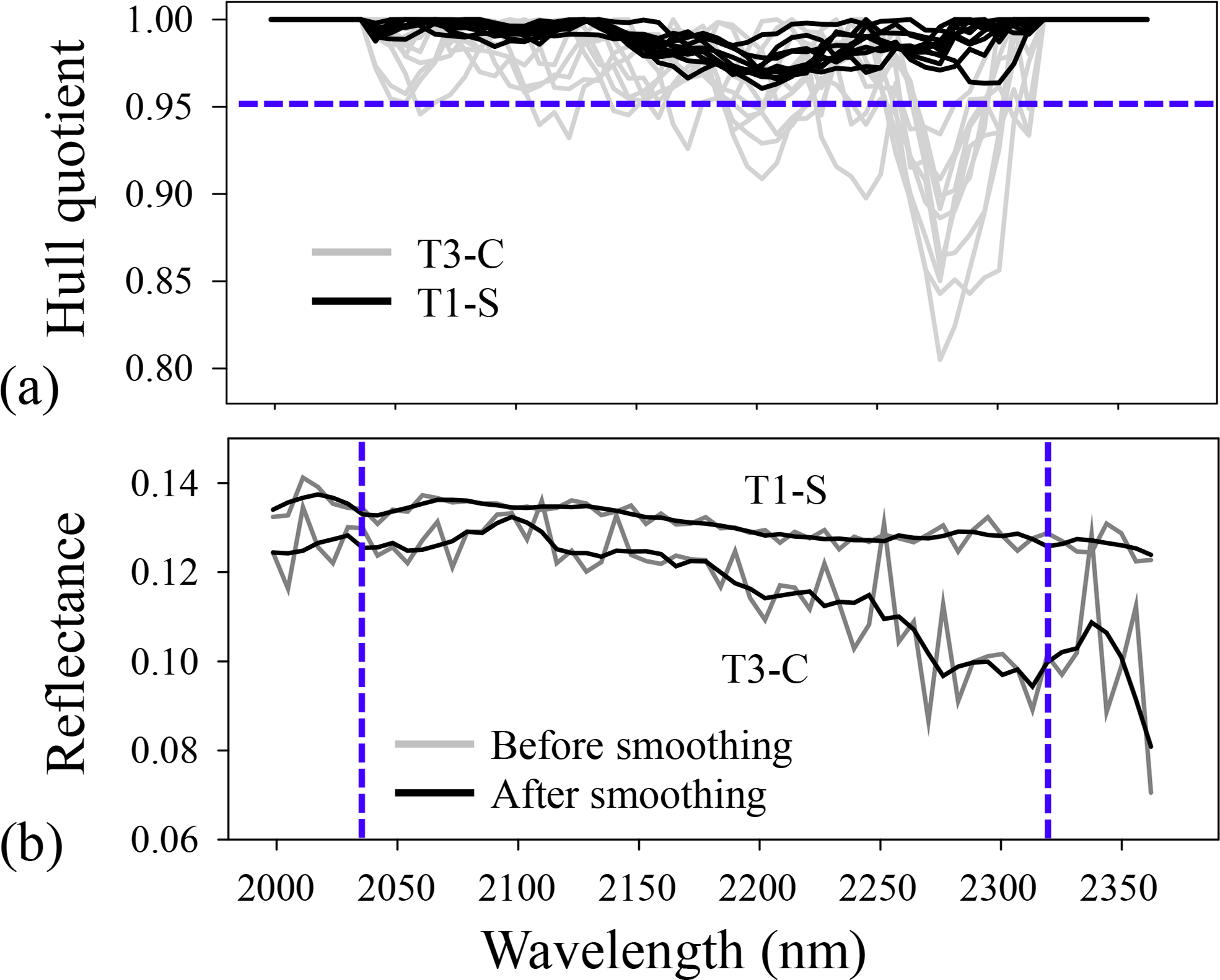
The peak in the numbers of pixels with an absorption feature at wavelengths greater than 2250 nm in image T3-C was investigated further. It was not known whether this peak was caused by noise or as a result of subtle mineral absorption features becoming more pronounced under the more diffuse illumination conditions under which T3-C was acquired. The modal peak in this wavelength region was at 2276 nm (indicated in Figure 4). Pixels with absorption features at 2276 nm were identified in the wavelength parameter image derived from T3-C. A random selection of these pixels was extracted from images T1-S and T3-C; in each case the same image pixels were used (n = 10). The extracted spectra comprised hull quotients spectra and reflectance spectra from images before and after spectral smoothing (Figure 5). This was done to determine if the smoothing process had introduced spectral artefacts. Hull-quotients spectra from T1-S had a relatively flat spectral profile but the same pixel spectra from T3-C showed distinct dips in reflectance at wavelengths greater than 2250 nm (Figure 5a). No spectra from T1-S had absorption features which had values less than 0.95 (the depth threshold value used to identify absorption features). Spectra from T3-C did, however, have “features” which extended below the depth threshold, particularly around 2276 nm. Reflectance spectra from corresponding pixels from the unsmoothed and smoothed imagery showed no coherent absorption features in image T1-S (Figure 5b). In image T3-C, however, the same pixels showed a broad dip in reflectance at wavelengths greater than 2250 nm (Figure 5b). This indicated that for image T3-C absorptions at about 2276 nm, and other wavelengths longer than 2250 nm, were caused by factors which are unrelated to the mineralogy of the mine face.
The frequency distributions of pixels representing feature depth were similar for images T1-S, T2-S and T4-S (Figure 4). Image T3-C showed a different distribution, with the modal value and right side of the distribution shifted to greater values. The frequency distribution of pixel values representing the width parameter was similar for images T1-S and T2-S. The modal value was similar for both images (67 nm), as was the range of values. In contrast, images T3-C and T4-S showed a more marked bimodal distribution with a peak at 67 nm comprising a more distinct secondary peak at about 30 nm. This indicated that a proportion of pixels had absorption features which were narrower compared with T1-S and T2-S. Further examination revealed these features to be associated with noise in pixels which had not been excluded from consideration by the depth threshold.
3.1.2. Changes in Absorption Feature Parameters at Specific Wavelengths
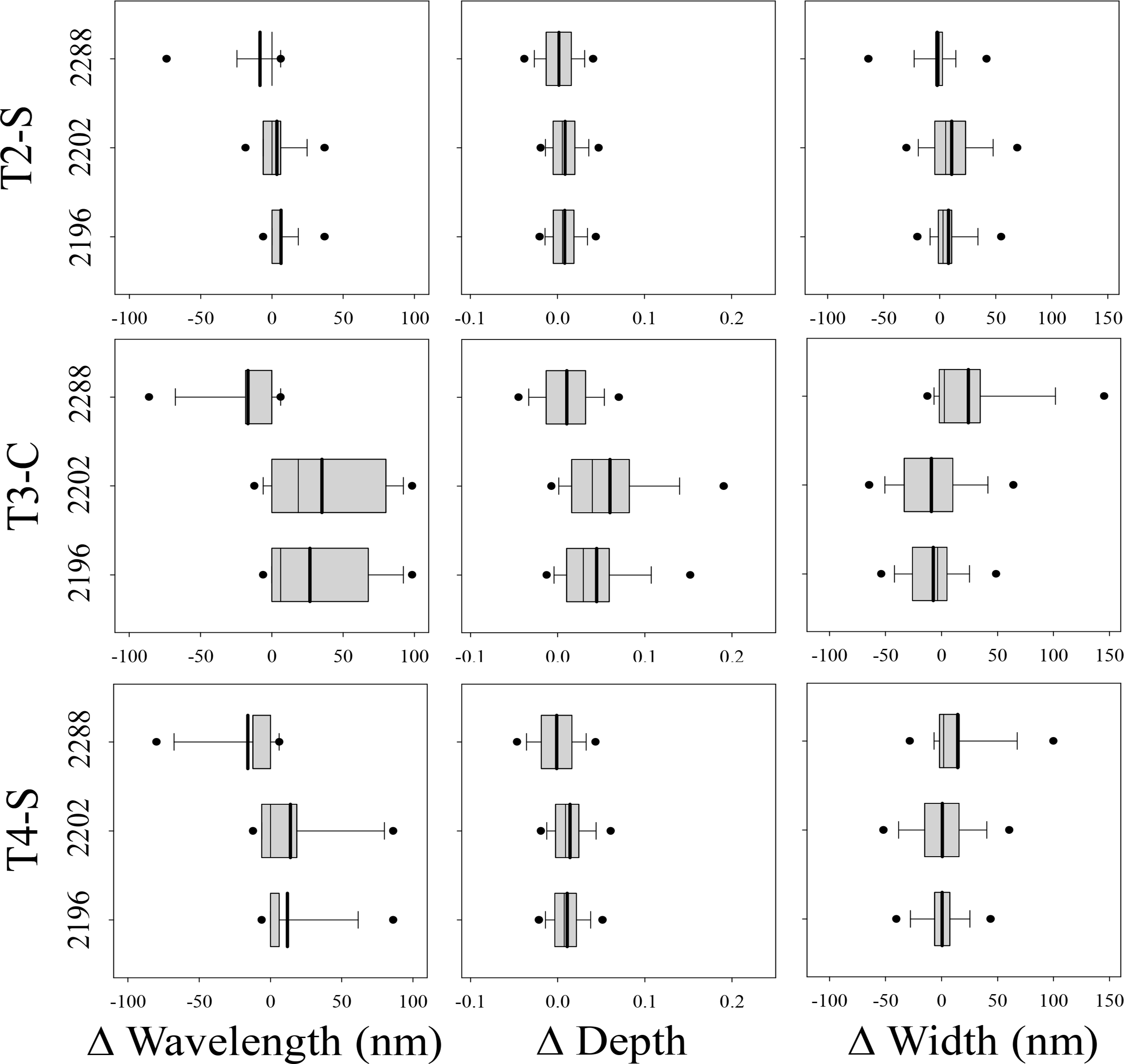
Absorption feature parameters in images T2-S, T3-C and T4-S changed in relation to those in image T1-S (Figure 6; Table 4). Wavelength positions of absorption features associated with kaolinite (centered on 2196 nm and 2202 nm) and nontronite (centered on 2288 nm) were, respectively, greater and smaller than the absorption features found in the same pixels in the baseline image (T1-S; Figure 6, Table 4). In all cases, this effect was more pronounced in the image acquired under cloud (T3-C). Changes in wavelength position were also more variable in T3-C than for images acquired in direct sunlight (T2-S and T4-S). The depth of all absorption features generally increased in all images relative to T1-S, with the greatest increase found for image T3-C. In comparison, changes in depth for images T2-S and T4-S were relatively small. Of the three measured parameters, changes in absorption feature width showed the greatest inconsistencies among different absorption features and images. For the features associated with kaolinite, width increased in T2-S and T4-S but decreased in T3-C. The feature associated with nontronite, showed a small decrease in width in T2-S but a relatively large increase in T3-C and T4-S. In general the largest changes in all feature parameters were found for the image acquired under cloud (T3-C) and the smallest for the image acquired under direct sunlight (T2-S, i.e., under similar illumination conditions to the baseline image T1-S.
3.1.3. Experiment 2—Spatial Patterns of Clay Absorption across Images
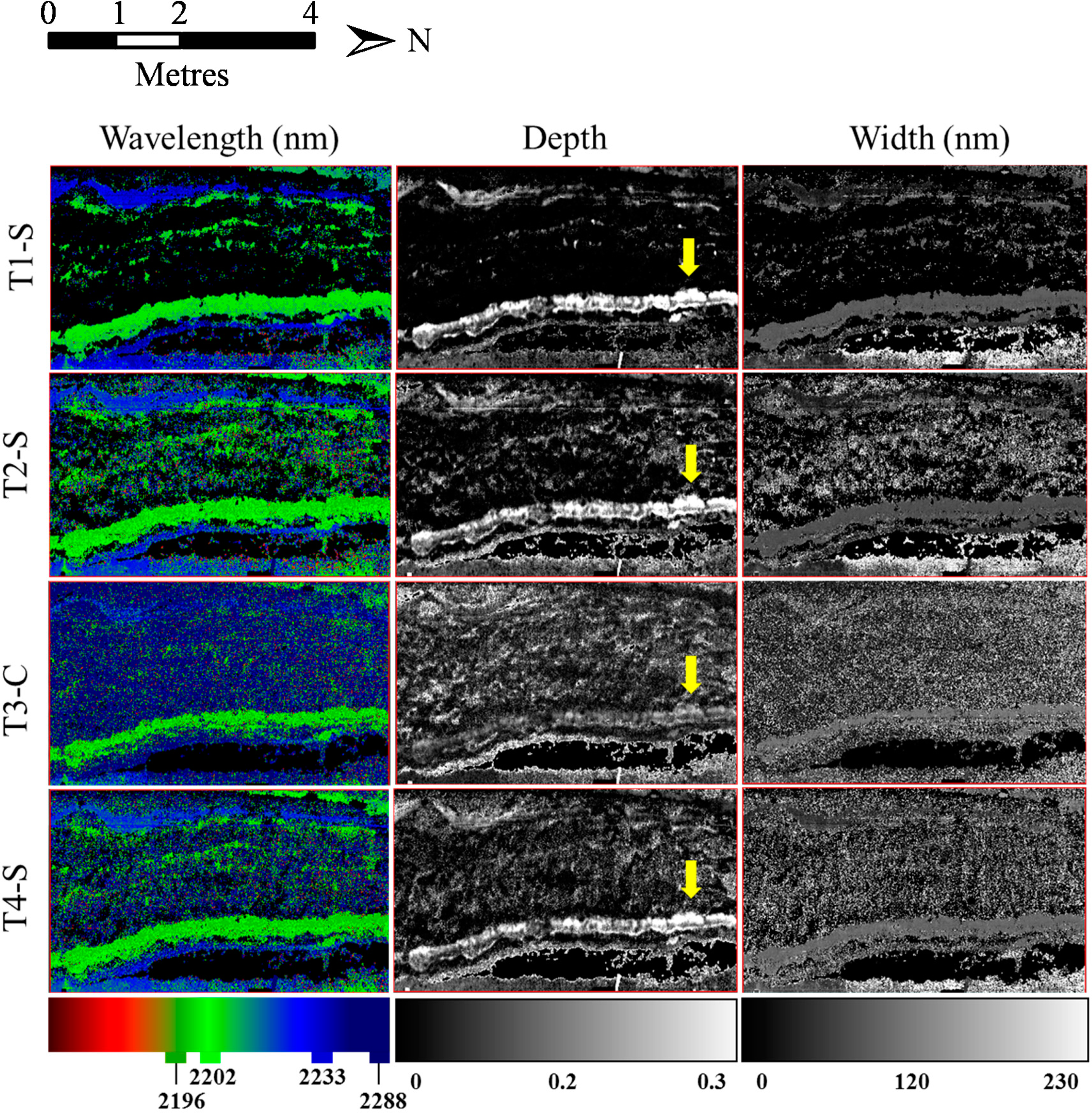
The proportion of total pixels in image Subset 1 identified by AFE as having a coherent absorption feature, as defined by the depth threshold, differed among images: T1-S (38%), T2-S (61%), T3-C (89%) and T4-S (72%). Images describing each absorption feature parameter were different among the replicate images (Figure 7).
For wavelength position, images T1-S and T2-S showed results that were largely consistent (i.e., spatial patterns mapped by wavelength position were similar in both images). This was unsurprising because these images were acquired under similar conditions of illumination. Spatial patterns in wavelength position shown in T1-S were largely preserved in T2-S; however, more pixels were identified by AFE in T2-S as having coherent absorption features. T1-S, T2-S and T4-S showed consistent, prominent layers of clay with absorption features at 2196 nm, 2202 nm and 2233 nm. Spatial patterns of wavelength position in T3-C were, however, very different to other images. Absorption features that were within the depth threshold value (i.e., a value of 0.95 or less in the hull quotients spectrum) were found in the great majority (89%) of image pixels. Although absorptions at 2202 nm still formed clear spatial patterns in some parts of the image, it is difficult to distinguish layers of clay in other parts of the image. Image T3-C has many more pixels with the longest wavelength (2288 nm) compared with other images and this is consistent with results from the frequency distributions (Experiment 1; Figure 4).
Pixels describing absorption feature depth in T1-S, T2-S and T4-S showed similar spatial patterns with respect to their intensity (brightness), with values in each image increasing in proportion with those in other images. For example, an area of intense absorption (indicated by arrows in Figure 7) of similar shape and extent is present in T1-S, T2-S and T4-S. Pixel values in this area are also greater (brighter) than other pixels in the same image. Image T3-C showed a different spatial pattern to all other images. For example, in the area of intense absorption (indicated by arrows in Figure 7) pixel values were not greater than for other areas in the same image; neither did they form an area of similar shape or extent as was observed in other images.
Pixels describing absorption feature width that had the largest values (greatest width) were present in parts of the image which contained black shale (see Subset 1, Figure 1). SWIR spectra of black shale have very weak absorptions due to disordered kaolinite or vermiculite. The brightest pixels in images T1-S, T2-S and T4-S had widths which exceeded 150 nm. The weak absorption features in black shale could not account for these large values. Further inspection indicated that spectral noise, particularly at longer wavelengths (>2300 nm), was the cause of the anomalously large values. Black shale had a reflectance of <8%, so that pixel values over the shale had small signal-to-noise ratios. The hull-quotients procedure used to normalize the spectra further increased noise, resulting in absorption features which were entirely an artefact of noise. These features were sufficiently deep as to be included in the depth threshold. Image T3-C showed little spatial structure with regard to absorption feature width and contained mainly noise. Results from all images indicated that width was not a useful parameter for mapping clays in these particular data. It was not therefore used in the subsequent analysis.
3.2. Experiment 3—Delineation and Quantification of Clay Layers across the Entire Mine Face
3.2.1. Clay Layers in Imagery
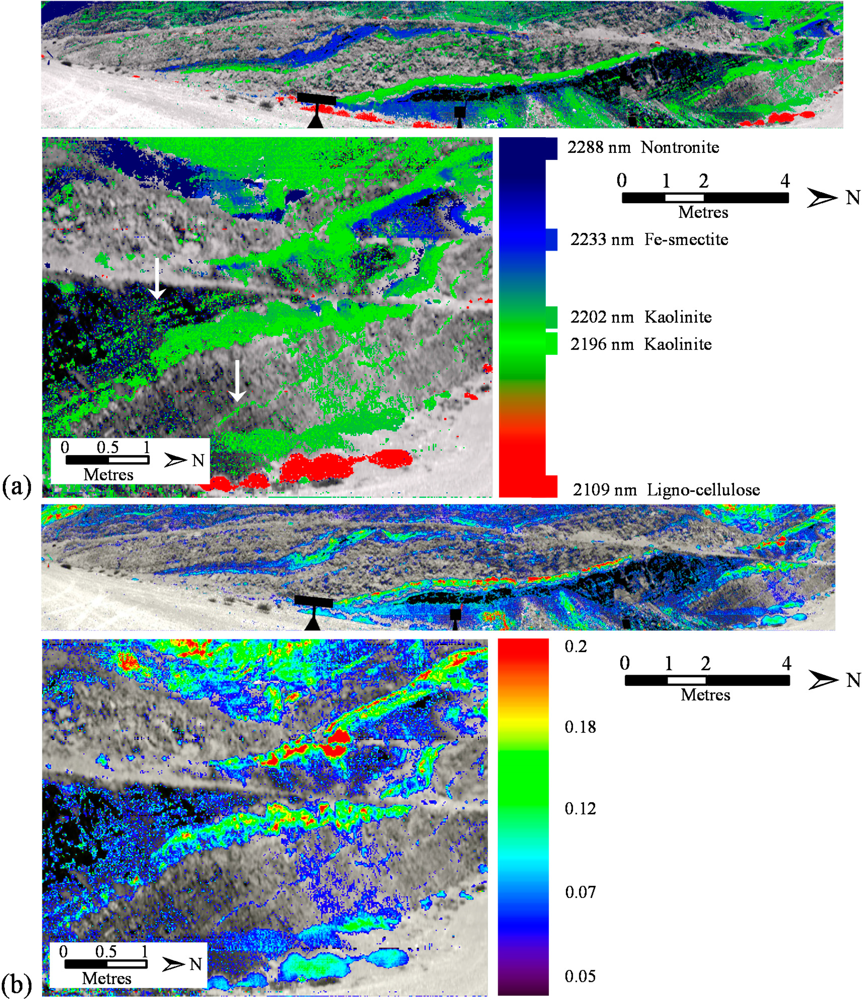
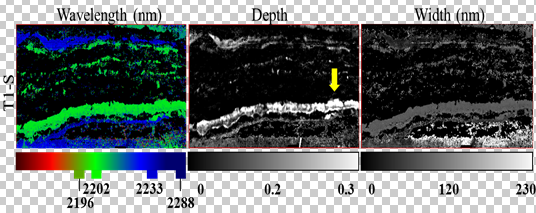
Images of wavelength position showed the presence of many layers of different types of clay of variable widths and lengths (Figure 8a). The depth of absorption features, as described by the depth parameter image were very variable spatially (Figure 8b). The deepest absorption features were related to kaolinite nontronite and Fe-smectite absorption features (cf. ( http://en.wikipedia.org/wiki/Cf.), Figure 8a,b). The clay layers in the image that were found by AFE were spatially coincident with the position of major clay layers recorded from the field survey (arrows in Figure 1) and with the predictions made from quantitative XRD of rock samples (see Section 3.2.2 and plot locations in Figure 1b). Several thin (2–4 cm thick) layers of clay which were not observed in the field were identified on the mine face by AFE (arrows in Figure 8a).
3.2.2. Validation—Comparison of Spectra from Imagery Acquired in the Laboratory and in the Field
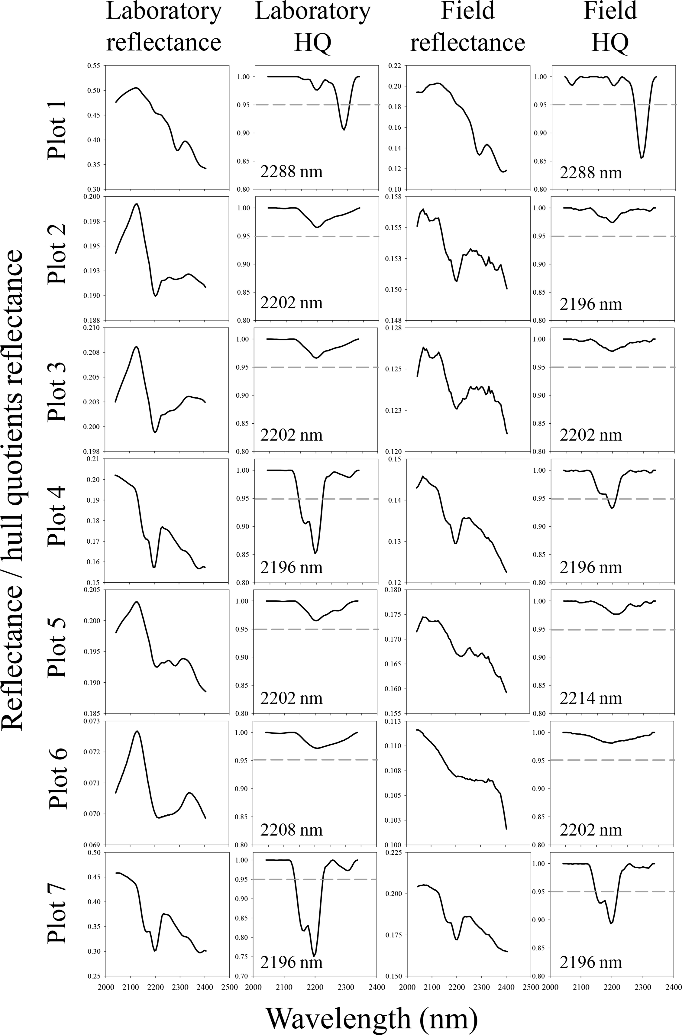
XRD analyses of samples taken from plots on the mine face revealed several minerals (Table 5) which have absorption features in the SWIR, as determined from the USGS and JPL spectral libraries: clinochlore (2325–2345 nm), nontronite (2284–2295 nm), kaolinite (2200–2205 nm) and vermiculite (2300–2325 nm). It was predicted that absorption features diagnostic of these minerals would be found in spectra in rocks from Plot 1 (nontronite), Plot 4 (kaolinite), Plot 6 (clinochlore, vermiculite) and Plot 7 (kaolinite). Amounts of kaolinite present in Plots 1, 3 and 6 were considered to be too small to cause absorption features of sufficient depth to be observed in image spectra or included in the depth threshold.
For validation, laboratory and field spectra were compared for each plot (Figure 9). Plots 1, 4, and 7 had absorption features which extended below the depth threshold and were therefore considered by AFE to have coherent absorption features. Plot 6 had a weak absorption above the depth threshold at 2208 and 2202 nm in the laboratory and field spectra, respectively. The wavelengths of these features were too short to be due to either clinochlore or vermiculite, but may be caused by some other minerals that were present but not quantified by XRD (note, the large amount of amorphous material for Plot 6; Table 5). This was most likely to be caused by amorphous silica [32,33]. XRD results for Plots 2, 3 and 5 did not reveal the presence of any minerals which might cause absorption in the SWIR, however, laboratory image spectra showed a weak feature located at 2202 nm. The wavelength of this feature in spectra from the field imagery was more variable but spectra had a similar shape to the laboratory image spectra. These results indicated that spectra acquired in the laboratory were consistent with spectra acquired from field imagery of the mine face. The clay minerals found in Plots 1, 4 and 7 were also consistent with those determined by XRD. Some absorption features presented in Figure 9 appeared to be real (e.g., Plots 2 and 3); they had a coherent shape comprising short- and long-wave slopes either side of a discrete reflectance minimum. However, these were not categorized as coherent features by AFE as they had minimal reflectances which were above the threshold (the dotted line in Figure 9). The apparent coherency of these features in Figure 9 arised from the fact that they were averages over the entire plot. Individual pixel spectra upon which AFE operated had more noise, and shallow absorption features could not be consistently distinguished from this background of noise. These features are therefore excluded from parameterization by AFE.
3.2.3. Absorption Features Mapped across the Whole Mine Face
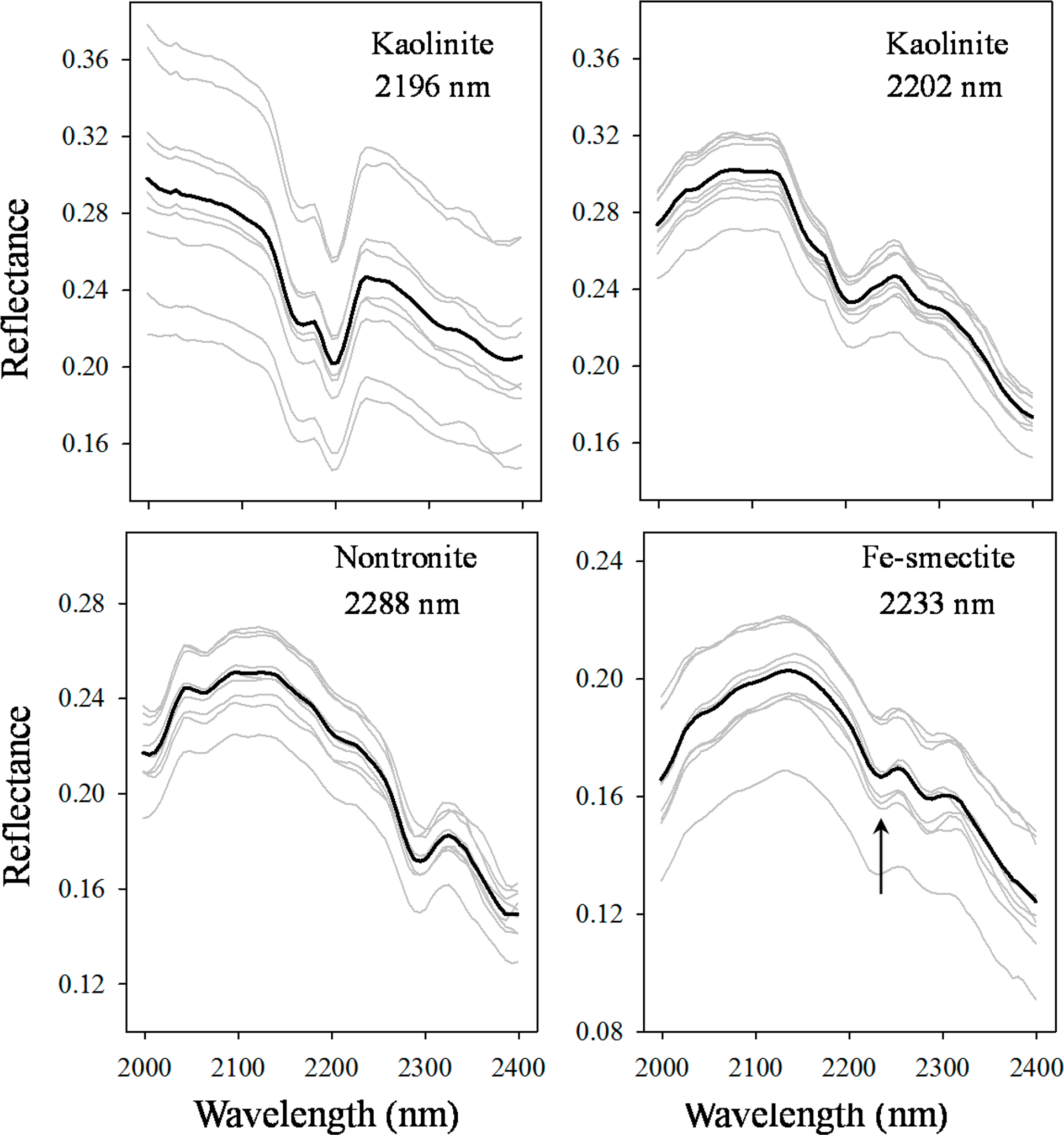
The deepest absorption features found in each pixel spectrum by AFE were located at wavelengths of 2109 nm (ligno-cellulose), 2196 nm and 2202 nm (kaolinite), 2233 nm (Fe-smectite) and 2288 nm (nontronite). The identity of the minerals causing these absorptions was determined using a combination of the XRD analyses (Table 5), the curve shape of the spectra and the wavelength locations of known mineral absorptions from the literature (Figure 10). Kaolinite was identified by its characteristic absorption doublet with a main absorption at about 2200 nm and a second absorption at about 2160 nm [20,21]. Spectra with absorption maxima at 2196 nm and 2202 nm either exhibited a discrete doublet or a shoulder at about 2160 nm. The difference in wavelength position between these two kaolinite features was small (a single spectral band); this may be due to a number of factors, including the amounts of impurities present at the location. Nontronite was distinguished by a pronounced absorption at 2288 nm caused by Fe-OH. [24]. Numerous pixels had an absorption at 2233 nm. Pixel spectra with an absorption at this wavelength also had an absorption between 2284 and 2288 nm. In reflectance spectra, the deepest of these features appears to be the one located to longer wavelengths (i.e., between 2284–2288 nm). However, after removal of the spectral continuum, the deepest feature was found to be located at 2233 nm. The wavelength locations of these absorptions is similar to those reported by [24] for Fe-smectite, specifically at 2288 nm and 2236 nm. We therefore assign the absorption at 2236 nm to Fe-smectite. In some spectra the 2284–2288 nm feature was deeper than the feature at 2233 nm in which case this suggested that the spectrum was dominated by nontronite. Spectra of pixels identified as having mineral absorption features at each of these wavelengths showed a consistent spectral shape but some had large variations in reflectance (Figure 10).
4. Discussion
Several laboratory studies have shown that parameters of absorption features, in particular wavelength position, can yield valuable information related to aspects of the chemical-physical properties of minerals [25,34]. Some studies have extracted meaningful information about mineralogy from the wavelength position of absorption features derived from airborne imagery, e.g., [35]. It remains, however, unclear as to the reproducibility of results when data are acquired of the same target but under different conditions of illumination or, in the case of imagery acquired from field-based platforms, under cloud. Changes in absorption feature parameters are a particular concern where data are acquired from topographically complex vertical surfaces such as mine faces or outcrops of rock. This is because changes in the position of the sun relative to the sensor and target can cause large spatial variations in incident and reflected light, thus complicating atmospheric correction.
In Experiment 1 we evaluated the effects of changing illumination conditions on feature parameters derived from imagery acquired from a topographically complex mine face. The feature parameters, wavelength position, depth and width were found to be similar for replicate imagery acquired under similar conditions of illumination and time of day. Feature parameters derived from imagery acquired under cloud (T3-C) were, however, different to those derived from imagery acquired under “optimal” conditions (direct sunlight; T1-S). Absorptions at shorter wavelengths, i.e., 2196 nm and 2202 nm, caused by kaolinite were, on average, shifted to longer wavelengths in T3-C. The opposite effect was found for the feature at 2288 nm, caused by nontronite which was, on average, shifted to shorter wavelengths in T3-C. On average, depth of all absorption features increased in T3-C compared with T1-S. Relative to T1-S, the width of absorption features in T3-S decreased for absorptions at 2196 nm and 2202 nm but increased in the absorption at 2288 nm. Some of these effects were observed, but to a smaller extent, in imagery acquired under very different solar angles (i.e., image T4-S).
A major difference between T3-C and T1-S was the introduction of an absorption feature at wavelengths long-wave of 2250 nm. Although the purpose of this paper was to describe rather than to explain the causes of changes in feature parameters, the introduction of this feature in spectra from image T3-C requires further comment. The feature could result from either an incomplete removal of atmospheric absorption features during the calibration to reflectance and/or an increase in noise towards longer wavelengths. Several atmospheric absorptions are located at wavelengths long-wave of 2250 nm. Atmospheric water has a weak absorption centered at about 2276 nm but also causes a progressive decline in atmospheric transmission long-wave of about 2298 nm. Methane has a very weak atmospheric absorption which peaks at about 2347–2377 nm. Nitrogen also has a very weak absorption between about 2246–2326 nm. The combined effects of these absorptions may remain in spectra because they have not been completely removed by the flat-field reflectance calibration. Furthermore, their combined absorptions cause a decrease in atmospheric transmission long-wave of about 2300 nm, reducing the amount of signal available to the sensor causing a decrease in the signal to noise ratio of the data. Calibration of imagery to reflectance was done using a simple flat-field approach which effectively removed multiplicative but not additive atmospheric effects such as scattered path radiance. Cloud cover increases scattered path radiance which can potentially reduce contrast, particularly for low albedo materials or surfaces under conditions of shade. Because the calibration panel is, nominally at least, illuminated by the same light as the mine face, atmospheric effects should have been removed by the calibration process. No residual atmospheric absorptions should be seen in the data. Parts of the mine face were, however, affected by shade (caused by overhanging rock) and changes in illumination and reflection imposed by the complex geometry of its surface. These effects were present to some extent in all of the images used in this study. The calibration panel was not affected by shade in any image. The wavelength-intensity distribution of light reflected from the calibration panel would likely have been different to that reflected from areas of shade in the image. This is an inherent limitation of using a calibration panel located at a particular point on a surface to calibrate all areas of the surface which may or may not be affected by shade. The apparently spurious absorption feature in T3-C long-wave of 2250 nm is likely to have been caused by a combination of incomplete removal of atmospheric absorption and a decrease in signal to noise towards longer wavelengths. Noise spikes towards longer wavelengths would be defined as the part of the upper convex hull and would therefore be set to unity in the hull-quotients spectrum. Thus, any small reduction in reflectance towards shorter wavelengths caused by incomplete removal of atmospheric absorption effects would result in an absorption feature which may appear to be coherent over several spectral bands.
Not all parts of the hull-quotients spectrum which had values less than unity could be considered to be absorption features. Features which had a hull-quotients reflectance value of less than 1 but greater than ∼0.95 could not be distinguished from the background noise of the spectrum. The use of a depth threshold enabled such features to be excluded from the analysis. This simple approach may have excluded some weak, but genuine, mineral absorption features. In Experiment 2 we examined if the spatial patterns of clay absorption features found in imagery acquired under optimal conditions were preserved in imagery acquired in similar and under different conditions of illumination. To do this, the same depth threshold (0.95) was applied in each case. The proportion of pixels determined by AFE to have absorption features (i.e., had a hull quotients reflectance less than 0.95) was least in imagery acquired under optimal conditions (T1-S; 38%) but increased in the replicate imagery acquired under similar conditions (T2-S; 61%) and again the image acquired with a very different solar elevation angle (T4-S; 72%). The largest proportion was found in the image acquired under cloud (T3-C; 89%). This increase in the proportion of pixels was due to increasing noise in the spectrum and is consistent with measurements of amounts of noise made from the imagery. The increase in the proportion of pixels having a depth threshold of less than 0.95 was greater in imagery acquired under cloud. The likely cause of this is the reduction in the solar irradiance curve towards longer wavelengths, thus decreasing the signal-to-noise ratio to the extent that noise caused some parts of the spectrum to extend below the threshold of 0.95. This effect, when combined with changes in the parameters of absorption features, degraded the spatial patterns of clay absorption in imagery acquired under cloud (Figure 7). The depth threshold largely excluded spurious absorption features caused by noise at wavelengths > 2250 nm in the image acquired under optimal conditions (T1-S). It was not, however, effective in removing these features in the image acquired under cloud T3-C. Spurious absorptions were also found in the image acquired under very different solar elevation angles (T4-S); the depth threshold was partially successful in excluding these. As a consequence of changes in solar elevation angles, compared to other images T4-S had a greater proportion of shade in some parts of the image. The partial success of the depth threshold reflected the partitioning of the data into areas of the mine face which were directly lit and shaded. The depth threshold was able to exclude pixels in areas which were directly illuminated but not pixels in areas of shade (and hence a smaller signal-to-noise ratio). Clearly, more sophisticated methods of detecting “true” or coherent absorption features need to be developed which do not rely on a simple depth threshold.
AFE was selected to map clay minerals because absorption feature parameters can be directly related to certain aspects of mineralogy and because it requires no spectral library or a priori knowledge of any particular mine face. Moreover, the shape of the SWIR spectral curve is largely determined by the composite suite of spectral features present. In this way, changes in absorption feature parameters in response to changing conditions of illumination can have a profound effect on spectral curve shape. Such changes have the potential to cause significant changes to the spectral curve independent of mineralogy, thus potentially reducing the efficacy of techniques of classification which rely solely on the use of a spectral library. The results of this study indicate that changes in illumination conditions can introduce spurious absorption features into spectra and change the absorption feature parameters wavelength position, depth and width. These effects are greatest for data acquired under conditions of cloud. Nevertheless, when acquired under suitable conditions, hyperspectral data can be used to map and quantify clay layers on vertical geological surfaces. This represents a significant step towards incorporating meaningful information on mineralogy into models of slope stability and to provide information to spatially separate or delineate the boundaries between geological units of similar visual or spectral appearance.
5. Conclusions
Using the automated feature extraction (AFE) method, the distribution, identity and abundance of clay minerals could be mapped on the mine face without the use of a spectral library, enabling thin layers of clay, to be distinguished and mapped. The ability to rapidly quantify aspects of mineralogy from short-wave infrared (SWIR) absorption features, without the use of a spectral library and without a priori knowledge is of significance to mining corporations and government organizations interested in mitigating risks of slope failure. This study has shown that even thin layers of clay can be mapped from hyperspectral imagery acquired in the field.
The spatial distribution of the clay layers as mapped by AFE was largely consistent for images acquired under direct solar illumination. Changes in absorption feature parameters associated with specific mineral absorption features occurred in all images, but by far the largest changes occurred in the image acquired under cloud. The proportion of pixels determined by AFE to have absorption features (i.e., had a hull quotients reflectance less than 0.95) increased from 38%, under direct solar illumination, to 89%, under cloudy conditions. Changing conditions of illumination caused by cloud cover can therefore change the conclusions drawn from maps of mineral distribution derived from hyperspectral imagery acquired in the field. This finding underlines the importance of acquiring data under direct solar illumination where spatial patterns are to be mapped from absorption feature parameters.
Furthermore, residual atmospheric absorption features combined with an increase in noise towards longer wavelengths resulted in spurious absorption features being found at wavelengths longer than 2250 nm, with a modal peak at 2276 nm in imagery acquired under cloud. This finding has implications for quantifying SWIR absorption features, particularly when located towards longer wavelengths, from imagery acquired from field-based platforms.
This study is unique in the context of hyperspectral imagery acquired from field-based platforms, in that it characterizes detailed changes in mineral absorption feature parameters in response to changes in illumination. The findings from this study show that absorption feature parameters can change in response to changing illumination conditions. Changes in the parameters of individual absorption features together with the introduction of spurious absorption features towards longer wavelengths can have a significant impact upon the general shape of the SWIR spectral curve. Thus, the changes in feature parameters highlighted by this study also have implications for mapping minerals using spectral libraries using SAM or other spectral matching algorithms.
It is clear from this study that residual atmospheric absorption features and increased noise towards longer wavelengths can affect hyperspectral imagery acquired from field based platforms. The overarching conclusion of this study is that hyperspectral imagery acquired in the field, when used to quantify SWIR absorption features, should be collected under direct solar illumination. The rapidly expanding field of field-based remote sensing would benefit significantly from an assessment of the relative efficacies of different approaches to calibration such as the empirical line method (using two calibration panels of different brightness) and atmospheric modeling using information contained within the data themselves.
Acknowledgments
This work has been supported by the Rio Tinto Centre for Mine Automation and the Australian Center for Field Robotics. The authors are grateful to Dr Andres Hernandez for his assistance in the laboratory.
Author Contributions
Richard Murphy was the principal investigator and was responsible for conceiving and designing the experiments, analyzing the data and preparing the manuscript. Sven Schneider and Sildomar Monteiro acquired the data and provided input into aspects of the data analysis.
Conflicts of Interest
The authors declare no conflict of interest.
References
- Morris, R.C. A textural and mineralogical study of the relationship of iron ore to banded iron-formation in the Hamersley Iron Province of Wester Australia. Econ. Geol 1980, 75, 184–209. [Google Scholar]
- Harmsworth, R.A.; Kneeshaw, M.; Morris, R.C.; Robinson, C.J.; Shrivastava, P.K. BIF-derived iron ores of the Hamersley Province. Geology of the Mineral Deposits of Australia and Papua New Guinea, Hughes, F.E., Ed.; The Australasian Institution of Mining and Metallurgy, Melbourne, Australia, 1990, 617–642. [Google Scholar]
- Hancox, G.T. The 1979 Abbotsford Landslide, Dunedin, New Zealand: A retrospective look at its nature and causes. Lansdslides 2008, 5, 177–188. [Google Scholar]
- Cornforth, D.H. Landslides in Practice: Investigation, Analysis, and Remedial/Preventative Options in Soils; Wiley & Sons: Hoboken, NJ, USA, 2005. [Google Scholar]
- Hutchinson, J.N. A landslide on a thin layer of quick clay at Furre, Central Norway. Geotechnique 1961, 11, 69–94. [Google Scholar]
- Hawkins, A.B. The significance of clay mylonites for slope stability. Proceedings of the First European Conference on Landslides, Prague, Czech Republic, 24–26 June 2002.Rybar, J., Stemberk, J., Wagner, P., Eds.; Taylor and Francis: Prague, Czech Republic, 2002; pp. 3–22.
- Stimpson, B. The magnitude of displacement almong clay mylonite shear zones. Q. J. Eng. Geol. Hydrogeol 1983, 16, 83–84. [Google Scholar]
- Goetz, A.F.H.; Chabrillat, S.; Lu, Z. Field reflectance spectrometry for detection of swelling clays at construction sites. F. Anal. Chem. Technol 2001, 5, 143–155. [Google Scholar]
- Gill, J.D.; West, M.W.; Noe, D.C.; Olsen, H.W.; McCarty, D.K. Geologic control of severe expansive clay damage to a subdivision in the Pierre Shale, Southwest Denver Metropolitan area, Colorado. Clays Clay Miner 1996, 44, 530–539. [Google Scholar]
- Moore, R. The chemical and mineralogical controls upon the residual strength of pure and natural clays. Geotechnique 1991, 41, 35–47. [Google Scholar]
- Chabrillat, S.; Goetz, A.F.H.; Krosley, L.; Olsen, H.W. Use of hyperspectral images in the identification and mapping of expansive clay soils and the role of spatial resolution. Remote Sens. Environ 2002, 82, 431–445. [Google Scholar]
- Griffiths, D.V.; Lane, P.A. Slope stability analysis by finite elements. Geotechnique 2009, 49, 387–403. [Google Scholar]
- Kruse, F.A.; Lefkoff, A.B.; Boardman, J.B.; Heidebrecht, K.B.; Shapiro, A.T.; Barloon, P.J.; Goetz, A.F.H. The spectral image processing system (SIPS)—Interactive visualization and analysis of imaging spectrometer data. Remote Sens. Environ 1993, 44, 145–163. [Google Scholar]
- Clark, R.N.; Swayze, G.A.; Livo, K.E.; Kokaly, R.F.; Sutley, S.J.; Dalton, J.B.; McDougal, R.R.; Gent, C.A. Imaging spectroscopy: Earth and planetary remote sensing with the USGS Tetracorder and expert systems. J. Geophys. Res.: Planet 2003, 108, 5131. [Google Scholar]
- Ellis, R.J.; Scott, P.W. Evaluation of hyperspectral remote sensing as a means of environmental monitoring in the St. Austell China clay (kaolin) region, Cornwall, UK. Remote Sens. Environ 2004, 93, 118–130. [Google Scholar]
- Ferrier, G.; White, K.; Griffiths, G.; Bryant, R.; Stefouli, M. The mapping of hydrothermal alteration zones on the island of Lesvos, Greece using an integrated remote sensing dataset. Int. J. Remote Sens 2002, 23, 341–356. [Google Scholar]
- Murphy, R.J.; Monteiro, S.T.; Schneider, S. Evaluating classification techniques for mapping vertical geology using field-based hyperspectral sensors. IEEE Trans. Geosci. Remote Sens 2012, 50, 3066–3080. [Google Scholar]
- Kruse, F.A. Use of airborne imaging spectrometer data to map minerals associated with hydrothermally altered rocks in the northern Grapevine Mountains, Nevada, and California. Remote Sens. Environ 1988, 24, 31–51. [Google Scholar]
- Murphy, R.J. The effects of surficial vegetation cover on mineral absorption feature parameters. Int. J. Remote Sens 1995, 16, 2153–2164. [Google Scholar]
- Clark, R.N.; King, T.V.V.; Klejwa, M.; Swayze, G.A. High spectral resolution reflectance spectroscopy of minerals. J. Geophys. Res 1990, 95, 12653–12680. [Google Scholar]
- Hunt, G.R. Near-infrared (1.3–2.4) µm spectra of alteration minerals—Potential for use in remote sensing. Geophysics 1979, 44, 1974–1986. [Google Scholar]
- Van der Meer, F. Analysis of spectral absorption features in hyperspectral imagery. Int. J. Appl. Earth Obs. Geoinf 2004, 5, 55–68. [Google Scholar]
- Kruse, F.A.; Lefkoff, A.B.; Dietz, J.B. Expert system-based mineral mapping in northern Death Valley, California/Nevada, using the airborne visible/infrared imaging spectrometer (AVIRIS). Remote Sens. Environ 1993, 44, 309–336. [Google Scholar]
- Bishop, J.L.; Lane, M.D.; Dyar, M.D.; Brown, A.J. Reflectance and emission spectroscopy study of four groups of phyllosilicates: Smectites, kaolinite-serpentines, chlorites and micas. Clay miner 2008, 43, 35–54. [Google Scholar]
- Martínez-Alonso, S.; Rustad, J.R.; Goetz, A.F.H. Ab initio quantum mechanical modeling of infrared vibrational frequencies of the OH group in dioctahedral phyllosilicates. Part II: Main physical factors governing the OH vibrations. Am. Mineral 2002, 87, 1224–1234. [Google Scholar]
- Clark, R.N. Spectroscopy of rocks, and minerals and principles of spectroscopy. In Remote Sensing for the Earth Sciences, Manual of Remote Sensing, third ed; Rencz, A.N., Ryerson, R.A., Eds.; John Wiley & Sons: New York, NY, USA, 1999; Volume 3, pp. 3–58. [Google Scholar]
- Goetz, A.F.H. Three decades of hyperspectral remote sensing of the Earth: A personal view. Remote Sens. Environ 2009, 113, S5–S16. [Google Scholar]
- Morris, R.C.; Kneeshaw, M. Genesis modelling for the Hamersley BIF-hosted iron ores of Western Australia: A critical review. Aust. J. Earth Sci 2011, 58, 417–451. [Google Scholar]
- Savitzky, A.; Golay, M.J.E. Smoothing and differentiation of data by simplified least squares procedures. Anal. Chem 1964, 36, 1627–1639. [Google Scholar]
- Clark, R.N.; Roush, T.L. Reflectance spectroscopy: Quantitative analysis techniques for remote sensing applications. J. Geophys. Res 1984, 89, 6329–6340. [Google Scholar]
- Rodger, A.; Laukamp, C.; Haest, M.; Cudahy, T. A simple quadratic method of absorption feature wavelength estimation in continuum removed spectra. Remote Sens. Environ 2012, 118, 273–283. [Google Scholar]
- Goryniuk, M.C.; Rivard, B.A.; Jones, B. The reflectance spectra of opal-A (0.5–25 μm) from the Taupo Volcanic Zone: Spectra that may identify hydrothermal systems on planetary surfaces. Geophys. Res. Lett 2004, 31. [Google Scholar] [CrossRef]
- Milliken, R.E.; Swayze, G.A.; Arvidson, R.E.; Bishop, J.L.; Clark, R.N.; Ehlmann, B.L.; Green, R.O.; Grotzinger, J.P.; Morris, R.V.; Murchie, S.L.; et al. Opaline silica in young deposits on Mars. Geology 2008, 36, 847–850. [Google Scholar]
- Haest, M.; Cudahy, T.J.; Laukamp, C.; Gregory, S. Quantitative mineralogy from infrared spectroscopic data. I. Validation of mineral abundance and composition scripts at the rocklea channel iron deposit in Western Australia. Econ. Geol 2012, 107, 209–228. [Google Scholar]
- van Ruitenbeek, F.J.A.; Debba, P.; van der Meer, F.D.; Cudahy, T.; van der Meijde, M.; Hale, M. Mapping white micas and their absorption wavelengths using hyperspectral band ratios. Remote Sens. Environ 2006, 102, 211–222. [Google Scholar]


| Geological Unit | Plot | Description |
|---|---|---|
| CL1 | 1 | Clay layer, >5 m—thick, green-orange in color |
| A | 2,3 | Banded Iron Formation comprising hematite and Quartz, red in color |
| CL2 | 4 | Clay layer, ∼20 cm—thick, cream in color |
| B | 5 | Whaleback shale, more mineralized than A, comprising hematite and goethite with small amounts of quartz, red-orange in color |
| CL3 | 7 | Clay layer, ∼80 cm—thick, white to cream in color |
| C | 6 | Black shale, rich in clinochlore and vermiculite |
| D | - | Banded iron formation, red in color |
| Image | Local Time | Solar Elevation | Solar Zenith | Solar Azimuth | Illumination Condition |
|---|---|---|---|---|---|
| T1-S | 10:57 | 75.6 | 14.4 | 82 | Direct sunlight |
| T2-S | 11:18 | 80.4 | 9.6 | 75.6 | Direct sunlight |
| T3-C | 11:51 | 86.9 | 3.1 | 30.3 | Cloud |
| T4-S | 12:28 | 82.4 | 7.6 | 289.4 | Direct sunlight |
| Image | Spectralon (15%) | Teflon (∼80%) |
|---|---|---|
| T1-S | 0.27 | 2.70 |
| T2-S | 0.28 | 2.46 |
| T3-C | 0.24 | 1.26 |
| T4-S | 0.27 | 1.38 |
| (a) | (b) | ||||||
| Wavelength | Wavelength | ||||||
| Image | 2196 nm | 2202 nm | 2288 nm | Image | 2196 nm | 2202 nm | 2288 nm |
| T2-S | 6.328 | 3.466 | −8.393 | T2-S | 8.685 | 11.188 | 11.233 |
| T3-C | 26.674 | 35.097 | −16.673 | T3-C | 29.737 | 41.521 | 19.687 |
| T4-S | 11.932 | 14.037 | −15.848 | T4-S | 14.537 | 21.105 | 17.978 |
| (a) | (b) | ||||||
| Depth | Depth | ||||||
| Image | 2196 nm | 2202 nm | 2288 nm | Image | 2196 nm | 2202 nm | 2288 nm |
| T2-S | 0.008 | 0.009 | 0.002 | T2-S | 0.016 | 0.016 | 0.018 |
| T3-C | 0.045 | 0.060 | 0.010 | T3-C | 0.048 | 0.062 | 0.029 |
| T4-S | 0.011 | 0.014 | −0.001 | T4-S | 0.019 | 0.021 | 0.021 |
| Width | Width | ||||||
| Image | 2196 nm | 2202 nm | 2288 nm | Image | 2196 nm | 2202 nm | 2288 nm |
| T2-S | 7.795 | 10.632 | −2.319 | T2-S | 13.920 | 21.498 | 13.835 |
| T3-C | −7.248 | −9.045 | 23.986 | T3-C | 22.055 | 30.512 | 30.478 |
| T4-S | 0.442 | 0.642 | 14.449 | T4-S | 15.484 | 23.683 | 22.814 |
| Plot Number/Mineral | Plot 1 | Plot 2 | Plot 3 | Plot 4 | Plot 5 | Plot 6 | Plot 7 |
|---|---|---|---|---|---|---|---|
| Amorphous | 25.25 | 2.14 | 2.02 | 7.56 | 3.83 | 43.25 | 13 |
| Clinochlore | - | - | - | - | - | 36.5 | |
| Goethite | 60.5 | - | - | - | 22.75 | - | - |
| Hematite | 5.3 | 35.36 | 49.44 | 38.68 | 56.5 | - | - |
| Kaolinite | 3.88 | - | 0.62 | 53.8 | - | 1.63 | 87 |
| Nontronite | D | - | - | - | - | - | - |
| Quartz | 2.68 | 62.2 | 47.86 | - | 6.28 | 0.25 | - |
| Number of samples | 4 | 5 | 5 | 5 | 4 | 4 | 2 |
© 2014 by the authors; licensee MDPI, Basel, Switzerland This article is an open access article distributed under the terms and conditions of the Creative Commons Attribution license (http://creativecommons.org/licenses/by/3.0/).
Share and Cite
Murphy, R.J.; Schneider, S.; Monteiro, S.T. Mapping Layers of Clay in a Vertical Geological Surface Using Hyperspectral Imagery: Variability in Parameters of SWIR Absorption Features under Different Conditions of Illumination. Remote Sens. 2014, 6, 9104-9129. https://doi.org/10.3390/rs6099104
Murphy RJ, Schneider S, Monteiro ST. Mapping Layers of Clay in a Vertical Geological Surface Using Hyperspectral Imagery: Variability in Parameters of SWIR Absorption Features under Different Conditions of Illumination. Remote Sensing. 2014; 6(9):9104-9129. https://doi.org/10.3390/rs6099104
Chicago/Turabian StyleMurphy, Richard J., Sven Schneider, and Sildomar T. Monteiro. 2014. "Mapping Layers of Clay in a Vertical Geological Surface Using Hyperspectral Imagery: Variability in Parameters of SWIR Absorption Features under Different Conditions of Illumination" Remote Sensing 6, no. 9: 9104-9129. https://doi.org/10.3390/rs6099104