A Comparison of Model-Assisted Estimators to Infer Land Cover/Use Class Area Using Satellite Imagery


Abstract
: Remote sensing provides timely, economic, and objective data over a large area and has become the main data source for land cover/use area estimation. However, the classification results cannot be directly used to calculate the area of a given land cover/use type because of classification errors. The main purpose of this study is to explore the performance and stability of several model-assisted estimators in various overall accuracies of classification and sampling fractions. In this study, the confusion matrix calibration direct estimator, confusion matrix calibration inverse estimator, ratio estimator, and simple regression estimator were implemented to infer the areas of several land cover classes using simple random sampling without replacement in two experiments: a case study using simulation data based on RapidEye images and that using actual RapidEye and Huan Jing (HJ)-1A images. In addition, the simple estimator using a simple random sample without replacement was regarded as a basic estimator. The comparison results suggested that the confusion matrix calibration estimators, ratio estimator, and simple regression estimator could provide more accurate and stable estimates than the simple random sampling estimator. In addition, high-quality classification data played a positive role in the estimation, and the confusion matrix inverse estimators were more sensitive to the classification accuracy. In the simulated experiment, the average deviation of a confusion matrix calibration inverse estimator decreased by about 0.195 with the increasing overall accuracy of classification; otherwise, the variation of the other three model-assisted estimators was 0.102. Moreover, the simple regression estimator was slightly superior to the confusion matrix calibration estimators and required fewer sample units under acceptable classification accuracy levels of 70%–90%.
1. Introduction
The area of each land cover class is an essential parameter of resources investigation, resources management, and earth observation [1–5]. It also plays an important role in scientific understanding when dealing with environmentally sensitive policies [6]. During the past few decades, many operational area estimation projects have been launched for all land cover/use classes, such as the Land Use/Cover Area Frame Statistical Survey (LUCAS) [3], or for specific land cover/use classes (mainly agriculture and forestry, such as Agriculture and Resources Inventory Surveys through Aerospace Remote Sensing (AgRISTARS), Cropland Data Layer (CDL), and Monitoring Agriculture with Remote Sensing (MARS) [7]. Satellite imagery-based scientific inference and sampling technology have been indispensable components of the area estimation procedure.
Two different typical approaches are used for inference of area such as probability-based inference and model-based inference [8]. Probability-based inference, also known as design-based inference, is based on probability sampling and the validity of inference is based on the probabilistic nature of the sampling design [9]. All estimators that require probability samples are by definition probability-based estimators [10]. In this type of inference, satellite imageries are often used to improve the sample frame design [4]. Model-based inference uses models to predict the response variable for individual population units, and the sample could be non-probability and purposive [11]. It focuses on the parameters of the superpopulation, and the validity of estimates depends on the fitness of model [9]. In this type of inference, satellite imageries are often used as auxiliary data or variables to establish the model. Model-assisted estimators are kinds of estimators that rely on models, however they fall in the category of probability-based estimators, such as simple random sampling, stratified, ratio estimators, because of their reliance on probability sampling [12]. These estimators take advantage of the correlation of the auxiliary variables and variables of interest from the probability sample to establish a model for improving the precision of the estimation, acting as a middle ground between the simple random sampling estimator and model-based estimator [8]. Additionally in these estimations, satellite imageries are usually viewed as key auxiliary data from which the auxiliary variables are derived. Confusion matrix calibration estimators, ratio estimators, and simple regression estimators are widely used model-assisted estimators.
The confusion matrix is a cross-tabulation of the classified category against the reference category or that observed in field survey at a specified location and is generally used to assess the accuracy of a classification [13]. The sample used to construct the confusion matrix reflects the ground truth condition and can be simultaneously input into estimators to implement the area estimation [5]. Initially, these estimators were regarded as a way to reduce or eliminate bias in pixel counting, which is performed by simply counting the pixels classified into the classes of interest and multiplying them by the area represented by each pixel [2,14,15]. Czaplewski and Catts [16] gave a more structured presentation. In the present study, we refer to these estimators as confusion matrix calibration estimators. Moreover, ratio and simple regression estimators are commonly used estimators, which are particular cases or extensions of the general regression estimator [10] with a strong basis in statistical theory and a long history of applications in various fields [17]. The general regression estimator usually explores and takes advantage of the reliable relationship between two datasets [18], such as satellite images and ground survey data, to reduce the variance.
Brun, et al. [19] applied regression and the confusion matrix calibration estimator to calculate crop areas and indicated that the relative efficiency of a confusion matrix calibration estimator is substantially lower than that of a regression estimator. However, they used different types of sample units during the estimation process—point sample units for confusion matrix calibration estimators and segment sample units for regression estimators—which may have introduced uncertainty to the conclusions. Gallego [2] provided a comprehensive review of various area estimation methods using remote sensing data and mainly probability-based estimators. Stehman [5] established model-assisted estimation as a unifying framework and pointed out a strong connection between accuracy assessment and area estimation for land cover or land cover change based on satellite imageries and compared and summarized a variety of confusion matrix calibration estimators [20]. McRoberts compared probability-based and model-based estimators based on logistic regression and remote sensing and inventory data to infer the proportion of forest [8], gave a systematic analysis about scientific inference using satellite imageries as auxiliary data [21], and implemented these estimators in many applications [22–27]. Foody [28] studied the impact of inaccurate ground reference data on the precision of land cover change area estimation in a simulation experiment and proved that the ground reference data imperfection can lead to a misestimation of land cover change area, the magnitude of which can be large when the area of land cover change is rare [29]. Olofsson, et al. [30] quantified the uncertainty in inferring the area of land cover change using stratified estimation by confidence interval.
Although many studies used the derived data from satellite imageries for classification or extraction of specified land cover class/use, the effects of accuracy of the derived data on the performance of some estimators is not clear. The objectives of our study are to compare the performances of different model-assisted estimators, and to analyze the impacts of the various qualities of classification on these estimators. We used the confusion matrix calibration direct estimator, inverse estimator, ratio estimator, and simple regression estimator to infer the areas of land cover classes based on different qualities of classification. Here, two case studies were conducted; one used simulated data, and the other used actual satellite images. The extents of the two study areas were viewed as two finite populations, and the regular segment was the sampling unit. The four model-assisted estimators and simple random sampling estimator were then implemented to infer the areas of land cover classes based on the different qualities of classification. Finally, the estimates of each land cover of classes were then compared.
2. Study Area and Data
2.1. Case Study Using Simulated Data
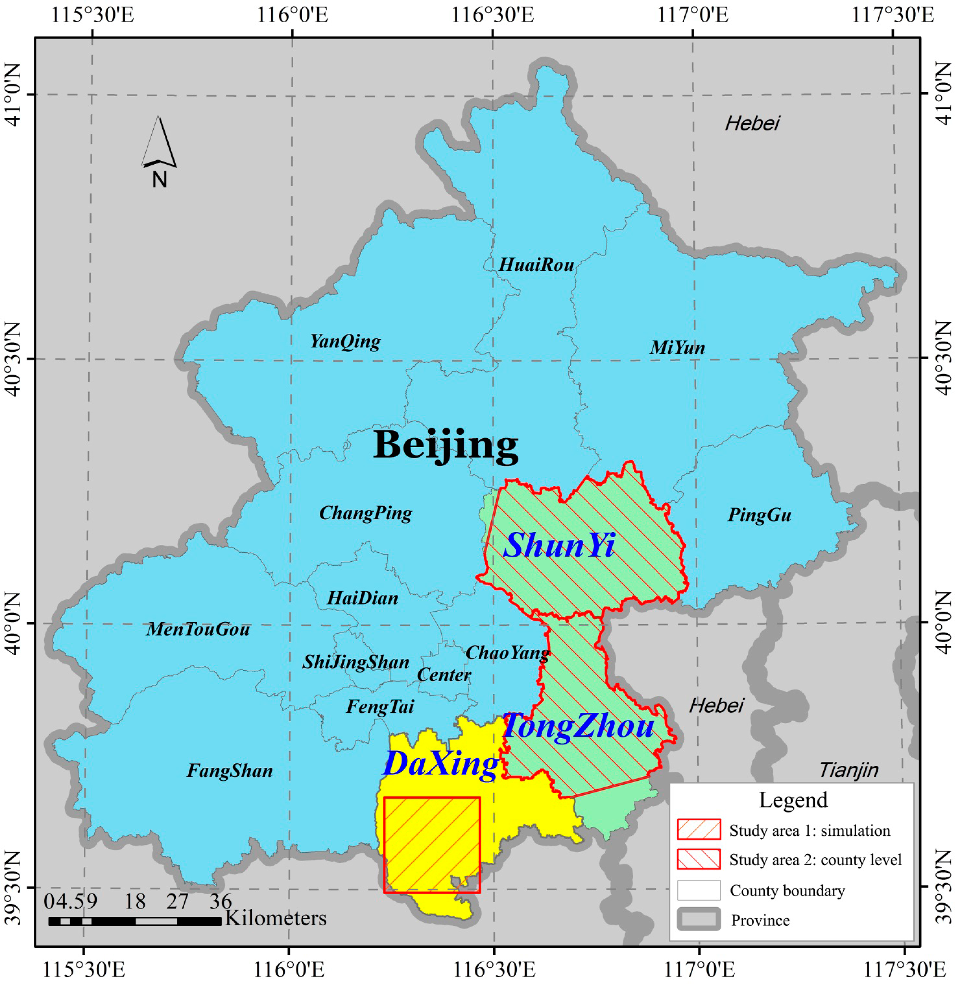
The area chosen for the simulation study was a square-shaped region with an area of 400 km2 (39°29′–39°40′N, 116°14′–116°28′E), hereafter referred to as study area 1, located in the Da Xing District of southern Beijing (Figure 1). Land cover classes for study area 1 are natural herbs dominated by sward and hydrophyte; crops dominated by maize; woods and built-up and bare lands. It is a rural–urban fringe zone with a fragmented landscape consisting of small, complex patches.
The data used in the simulated experiment were high-spatial resolution (5 m) images obtained on 13 September 2010, from RapidEye satellites equipped with the Jena-Optronik multi-spectral imager. The sensor is capable of collecting five distinct electromagnetic spectra: blue (0.44–0.51 μm), green (0.52–0.59 μm), red (0.63–0.69 μm), red-edge (0.69–0.73 μm), and near-infrared (0.76–0.88 μm). The spectral signatures of the five land cover classes previously mentioned are sufficiently distinct to support accurate classification. We used a support vector machine (SVM), a classifier defining a separating hyperplane based on supervised learning, to create the classification. In classification procedures, approximately 20 pixels of training samples in each land cover class were allocated based on interpretation, and a total of 104 pixels of training samples were input into the classifier. To evaluate the quality of the classification, all 16,000,000 pixels covering the entire study area 1 were viewed as the population. We selected 2000 pixels as a sample by simple random sampling without replacement. By interpreting the selected pixels one by one, we constructed the confusion matrix and calculated the overall accuracy [31]. The overall accuracy of classification (OA) is a main proportion measurement that ensures the pixel is correctly classified to describe the quality of a classification. As in this study, it is often derived from the confusion matrix with the diagonal elements (Table 1). The OA of SVM classification was 92%. In the simulated experiment, the SVM classification was used as a reference to validate and evaluate the performance of various estimators. To acquire different auxiliary data with various accuracies, we introduced classification errors into the reference data. Hereafter, the term auxiliary data will refer to the classification covering the entire area of interest; however, it could only provide inaccurate area information due to classification error or the relatively coarser spatial resolution. The term reference data is used to represent the images that describe the condition of ground truth or have less error and finer resolution to provide accurate area information. More details about the method of generating auxiliary data with different accuracies will be subsequently described in the Methods section.
2.2. Case Study Using Actual Remote Sensing Data
An operational case study was also implemented at two irregular regions, both in study area 2: TongZhou (TZ, 39°40′N–40°2′N, 116°31′E–116°57′E) and ShunYi districts (SY, 40°0′N–40°19′N, 116°28′E–116°59′E). It should be noted that a small fraction of these two districts was excluded because of limited image extent and cloud cover (Figure 1). These two regions cover approximately 788 km2 and 996 km2, respectively. In TZ, land cover types consist of winter wheat, grass, and wild rice shoots, wood, water, and built-up and bare lands. SY has the same land cover types, except for grass and wild rice shoots, although the landscapes are more fragmented and heterogeneous than those in TZ.
The datasets used in this section include the Huan Jing (HJ)-1A and RapidEye images obtained on 22 September 2010. The HJ-1 is a minisatellite constellation of China, and its main application fields are environmental monitoring and the prediction of land surface processing and disasters. HJ-1A is an optical satellite with a charge coupled device (CCD) camera and an infrared camera, and its repeat cycle is four days. HJ-1A imagery provides four optical bands including blue (0.43–0.52 μm), green (0.52–0.60 μm), red (0.63–0.69 μm), and near-infrared (0.76–0.90 μm), at 30 m resolution. The classification results via SVM from HJ images were used as auxiliary data; those from RapidEye images were used as reference data. Thus, the actual coverage of each category was known.
3 Methods
3.1. Simulation Procedure
Classification is well known to be incapable of providing a reliable estimate by the pixel counting method, which is performed by simply counting the pixels classified into the classes of interest, then multiplying by the area represented by each pixel [2], particularly on a large scale or in a fragmented landscape [1,32–34]. However, with a large coverage area, it offers synoptic information, which can be auxiliary data to estimation. The quality of classification, described by the main measurement of classification, overall accuracy, is an essential factor affecting estimator performance [35]. To evaluate the performance of each estimator under diverse auxiliary data quality, classifications with various accuracies are necessary. However, it is difficult to effectively control the accuracy in specified quantitative terms in the classification process. Thus, we generated simulated images. In this section, we introduce the rationale and steps of generation of simulated images.
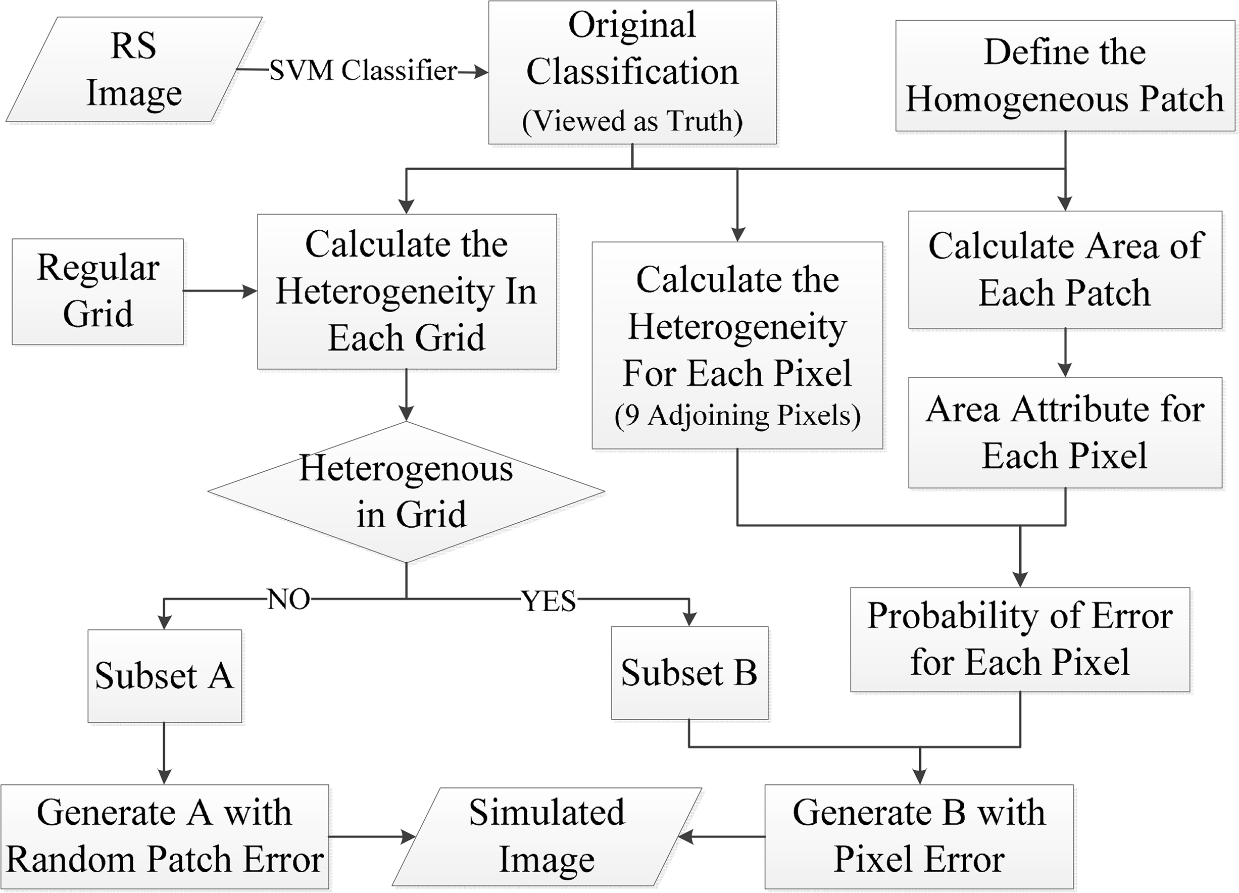
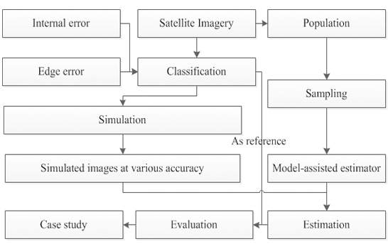
In the image simulation process, the original SVM classification obtained in Section 2.1 was used as reference data. We then created a classification error layer, and two types of errors [36] were simulated. One was the misclassification of pure pixels because of the similarity of their spectral signature [37], which is hereafter referred to as internal error. It is a commonly distributed inside feature and consists of several spatially contiguous pixels. Its occurrences depend on the degree of spectral separability. The more similar the spectral responses of the features, the more likely misclassifications are to occur. For example, misclassification between crops and grass is more common than that between crops and water. The other type of misclassification, containing several categories and occurring around the boundaries of different land cover/use classes, involves mixed pixels and is hereafter referred to as edge error. The simulation steps are described below and Figure 2 shows the workflow of simulation procedure.
- (1)
Definition of homogeneous patches: A homogeneous patch is a polygon, which is a contiguous area of homogeneous mapped land cover/use. Four neighboring pixels were used to define contiguity. A unique ID for each homogeneous patch was assigned and the logarithm transform by 10 of the area of each patch (expressed as x1) using its pixel count was calculated.
- (2)
Partition of “internal” and “edge” of patch: A window of 5 × 5 pixel size was used to overlay the reference imagery, and its center traversed every pixel in this step. If these pixels within the window belonged to the same land cover/use class, the central pixel was marked 1, representing an internal pixel; if not, the central pixel was marked 0, representing edge pixel. Finally, internal pixels comprised the internal area and edge pixels comprised the fringe area.
- (3)
Error simulation of internal area: This step generated an error layer inside the internal area. In our simulation, a sub-patch, with a fixed size was first set. The sub-patch could be any shape and size, as long as it was not larger than the smallest patch. It was necessary to ensure that the possibility of occurrence of sub-patch in any patch exists. Here, a regular sub-patch of 5 × 5 pixel size was used in our simulation. Then, we introduced a parameter, α, that could be set by users, expressing a proportion of error in the internal area. These error sub-patches were distributed randomly and their land cover/use classes might be anything except their reference.
- (4)
Error simulation of fringe area: The heterogeneity of each pixel in the fringe area, expressed as x2, was first calculated in eight neighboring pixels. Error probability for each pixel in the fringe area was then generated by Equation (1) [38]:
where p denotes the error probability for each pixel in the fringe area, β0, β1, β2 denote the coefficients of regression; the relation of regress was performed over all patches. It is notable that a high error probability for one pixel did not always indicate misclassification. For any pixel, supposing equation 1 gave a high error probability of this pixel; we could not determine if this pixel was an arbitrary error because the pixel can be classified correctly even if its error probability is high. Therefore, another parameter, c, was introduced to control the number of errors in the fringe area, which is a random digit between 0 and 1. If c was less than p, the pixel would be marked as an error, and its land cover/use class may be anything except the reference.- (5)
Simulated production: The errors generated in steps (3) and (4) were introduced into the reference to produce simulated images with various accuracy levels by adjusting parameters α and c. Finally, four simulated images were generated by injecting different quantitative errors. Hereafter, the simulated images were treated as the classification and also could be referred to as auxiliary data, and the original SVM classification was treated as the reference data. The overall accuracies of four simulated images were 62%, 70%, 80%, and 90%, respectively, representing the four classification levels (Figure 3).
3.2. Sampling Scheme and Samples
Generally, the following factors are considered for sampling design: (1) population; (2) sampling unit; and (3) sampling method and sampling fraction [39,40].
Here, the extents of the two study areas were viewed as two finite populations. Many studies and applications have been implemented using various types of sampling unit, points, segments (regular/irregular) and so on [39,41], they were feasible in these cases under certain conditions. To prevent confounding, we adopted the same area framework for the five estimators, and chose the sampling unit by considering its feasibility under the circumstance of using satellite imagery. In our study, the classification was crisp, and the point sampling unit was not suitable for discrete class labels due to the limitations of the traditional linear simple regression estimator (details about this estimator were introduced in Section 3.3). In contrast, for the two confusion matrix calibration estimators, we have a wider choice of sampling units [42,43]. Considering these factors, we used a regular segment of 80 m × 80 m as sampling unit. Because the comparison did not focus on the effect of the sampling method, a simple random sampling without replacement was implemented for convenience. We replicated the sample selection and estimation 2000 times for each classification by using different sample sizes ranging from 0.01% to 5.00%.
3.3. Estimators
3.3.1. Simple Random Sampling Estimator
Here, a simple random sampling estimator (SRSE) [8], which is a representative of the probability-based estimator, was implemented as a baseline for comparison [44] in the case study using simulated data and that using real remote sensing images.
The response variable, Y, is the area of land cover classes. Let Ŷs denote the estimation for class k of the SRSE; N, the number of all units; n, the sample size; and ȳ, the sample units means of reference data. The estimator of the total area of class k is
This estimator used the information from the sample only [26] and did not use the auxiliary data, which included simulated images and classification from HJ-1 in the case study using actual remote sensing data.
3.3.2. Model-Assisted Estimators
The confusion matrix is the core of the accuracy assessment process and provides an excellent summary of two types of classification errors, omission and commission [31]. Stehman [5] indicated that the reference information from a sample used to construct the confusion matrix can also be used to infer the area of the target directly or via model-assisted inference. The direct estimator (DIE) and inverse estimator (INE) are two approaches that utilize the confusion matrix to adjust the pixel count area. The difference between these two estimators is that the former employs the user’s accuracy, and the latter employs the producer’s accuracy. Assume the population consists of k classes: P denotes a population confusion matrix with k × k elements, and pij represents the proportion of pixels or the number of pixels, which are reference class i classified into class j (Table 1).
However, because the population confusion matrix is not available in the practical case, the estimated confusion matrix is based on the sample and possessing the same structure as the population confusion matrix, P̂, is an alternative. In addition, it was notable that we used simple random sampling without replacement to obtain a sample with a regular segment size of 80 m × 80 m that included 256 pixels in each selected segment. If we simply allocated the pixels covered by all segments and summarized their number or proportion accounting for total pixels to construct the common confusion matrix, the sampling would be cluster sampling rather than simple random sampling. Therefore, the reference information should be summarized by segment. We used the composite operator [45,46], which is widely used in the accuracy assessment of soft classification, to construct the confusion matrix. Using segment g as an example, we generated the confusion matrix for g segment following Equation (4), and the final confusion matrix, P̂, was built by averaging all segments of confusion matrices for entire selected segments.
Suppose a (k × 1) column vector t = (t1, t2,…, tk)′ represents the population area for each class in the reference data. This value is unknown and must be estimated. A (k × 1) column vector C = (C1, C2, …, Ck) represents the population area for each class in the auxiliary data and is easily obtained. R̂ denotes a diagonal (k × k) matrix, and diag(P̂′ 1) and T̂ denote diag(P̂1), where 1 denotes a (k × 1) column vector of 1’s. The direct and inverse estimators are expressed in the following forms by Stehman [5]:
Ratio estimator (RAE) and simple regression estimator (SRE) use variables that are correlated with variables of interest [12] and are widely used in many research fields [6,47]. Here, the simple regression estimator [20] was a representative of many forms of regression estimators and their transformations. The general forms of these two estimators are given by Equations (8) and (9):
3.4. Evaluation Criteria
Variance and standard error are common measurements for assessing the precision of estimators in statistical theory. For all estimators, the relation of their mean square error (MSE) and variance (V) can be expressed as
For an unbiased estimator, Bias(t)=0, and
Each sampling was considered an independent process, and each sample was entered into the five estimators. Considering the different area scales with various land cover classes and that the true value for every land cover class was known, we adopted the relative root mean square error (RRMSE) as the main evaluation criterion to compare the dispersion of estimations from its true area during 2000 iterations for each overall accuracy of classification and sample fraction. In addition, the reason for using RRMSE as in Chen and Wei’s [48] study was to compare the performances of these estimators directly and to examine the impact of overall classification accuracy on these estimators directly. It was noteworthy that the RRMSE of the area for every land cover class was calculated separately, and the results were added up to express the synthetic dispersion. The lower RRMSE for an estimator meant that the variability of estimations for 2000 iterations was smaller and that the estimator provided better performance. Moreover, the average deviation (AD) and coefficient of variance (CV) were also calculated. The former is an index assisting the expression of the variability of estimates for 2000 iterations, and the latter describes the similarity of the estimates from different samples. These evaluation criteria are defined as
4. Results and Discussion
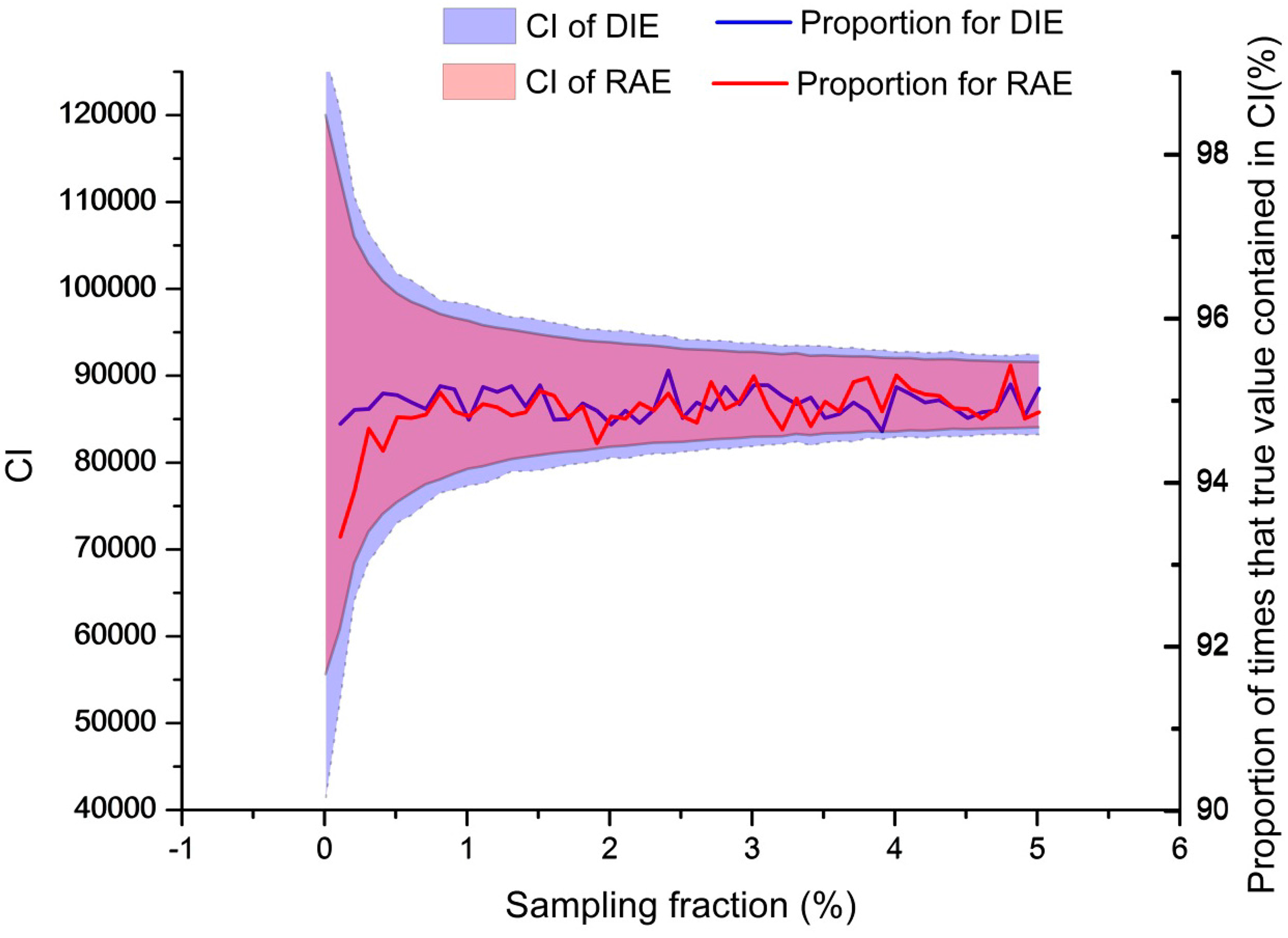
Variance estimation was implemented for these five estimators by Equations (3), (7), (10) and (11) before comparison. Meanwhile, the 95% confidence intervals (CI) (estimates plus and minus 1.96 times the square root of the variance estimates) were constructed to check if the proportion of times the simulation estimates contained the true area values was similar to the nominal coverage of 95% (Figure 4).
4.1. Results of Simulation Study
4.1.1. Comparison of Estimators across Various Classification Accuracy Levels
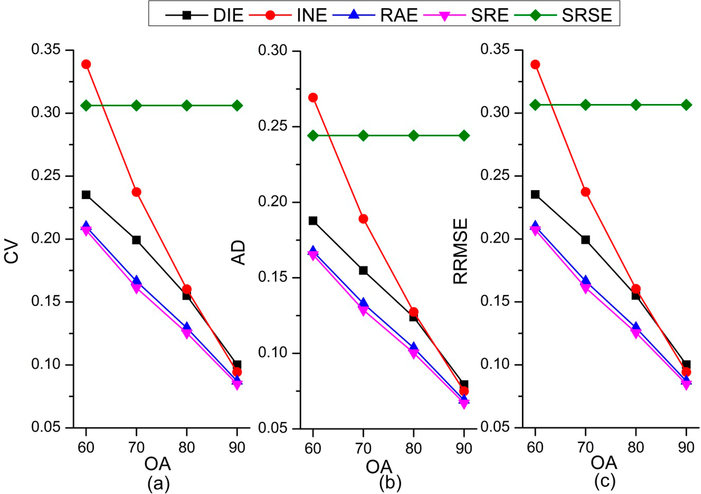
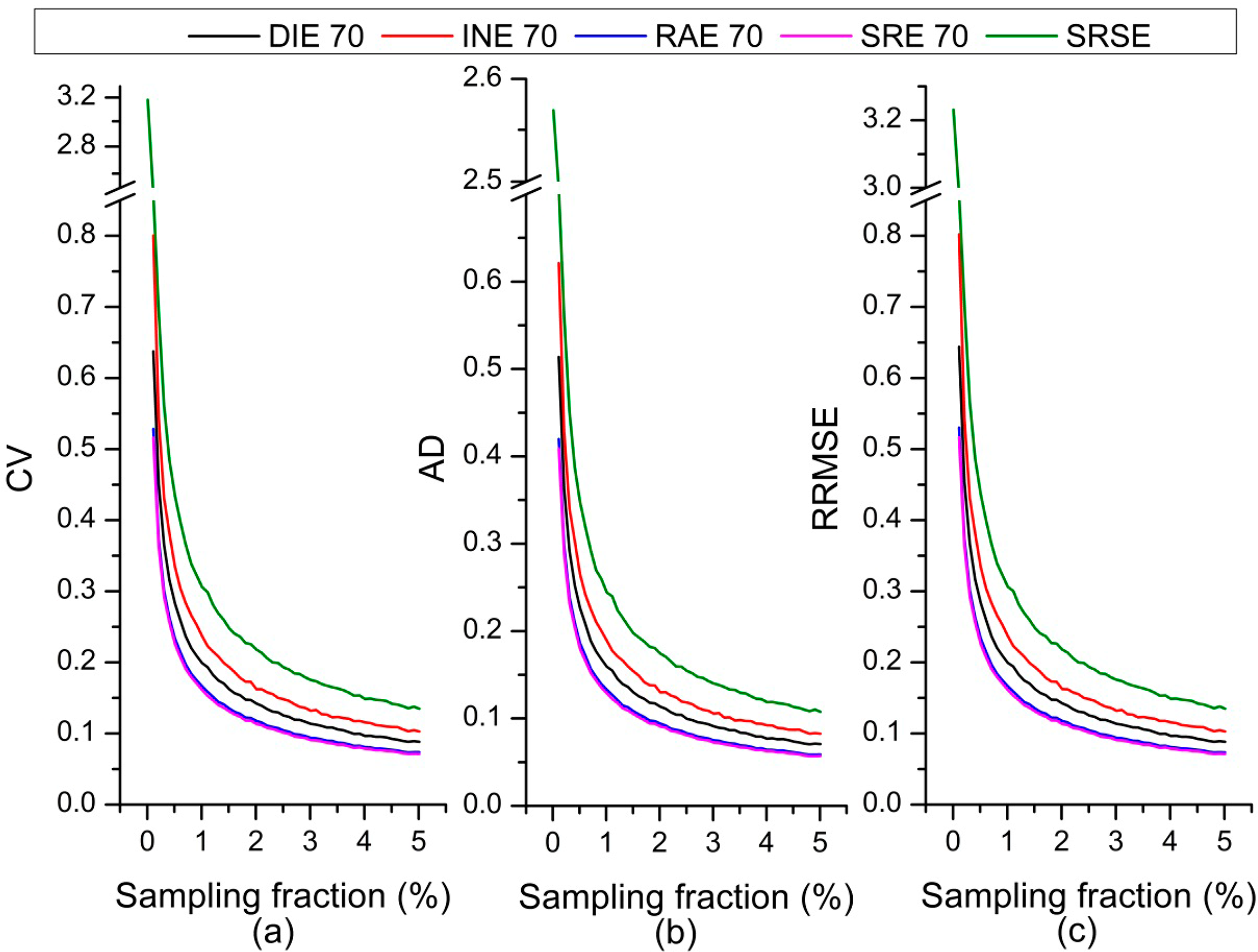
Figure 5 presents the variation of CV, AD, and RRMSE with various classification accuracy levels at 1% sampling fraction (about 625 sample units). SRSE is distinctive because it employs only the sample information rather than the auxiliary data. Thus, its CV, AD, and RRMSE are stable at 0.306, 0.244, and 0.307, respectively. Compared with the SRSE, almost all the other estimators have smaller CV, AD, and RRMSE values, which indicates that the auxiliary data benefits effective estimation. However, auxiliary data with low accuracy (62%) did not contribute to the reduction of CV, AD, and RRMSE for INE. When the auxiliary data has low accuracy (62%), the CV, AD, and RRMSE derived from INE is worse than that derived from SRSE. This means the low quality classification would damage or weaken the relationship between the auxiliary data and reference data and lead to an inaccurate estimation. Therefore, low quality classification might not play a positive role for estimation for certain estimators.
The four estimators except SRSE show a tendency of decreasing CV, AD, and RRMSE with increasing classification accuracy. We see that the regression group (RAE and SRE) is slightly superior to the confusion matrix calibration group at acceptable classification accuracy levels (70%–80%) with the smaller CV, AD, and RRMSE. When the accuracy exceeds a certain level (90%), the difference among these four estimators is slight. Considering that accurate classification (auxiliary data) is difficult to acquire, especially in large scales and complex landscapes, selecting an appropriate estimator is critical. Therefore, we suggest that SRE be given higher priority for operational use.
Although it is expected that CV, AD, and RRMSE decrease with an increase in classification accuracy, the extent of their variation with estimators differs. INE has the largest variation as the accuracy increases. The AD of a confusion matrix calibration inverse estimator decreased about 0.195 with increasing overall accuracy of classification; otherwise, the variation of the other three model-assisted estimators was about 0.102. The variations of the RAE and SRE are small and quite close. Therefore, the INE estimator is more sensitive than the other three estimators.
RAE and SRE methods use the information from sampling units, are more comprehensive and do care for the acreage of interested classes in sampling units. Also, the relationship between sample units and auxiliary data stands for the general connection between ground truth and satellite imageries classification. They also reduce the influence of each individual sample unit. The confusion matrix is interested not only in the number of pixels which are classified correctly, but also in which land cover/use type each error pixel is classified. In confusion matrix calibration methods, commission error portions are used to eliminate the area misclassified into the target classes, and the omission error portions are used to retrieve the area from the non-target classes. However, the classification errors are not randomly distributed over the interested region and classification matrix is not likely to describe the classification error for every class equally well. That means the precisions of estimation of target classes are likely to be affected by the precision of other classes and has more latent risk. Thus, the precision of estimation derived from confusion matrix calibration depends on how well the confusion matrix describes the error in each class.
4.1.2. Comparison of the Sample Size to Reach the Same Precision of Estimation
Increasing the sample size can be a method for improving the precision of estimation. However, the sample is supported by ground investigation or high spatial resolution imagery, which is labor intensive, time consuming, and costly. In practical cases, end users generally need to decrease the sample size and maximize benefits. Therefore, we also compared the sample size required by each estimator in a fixed precision of estimation.
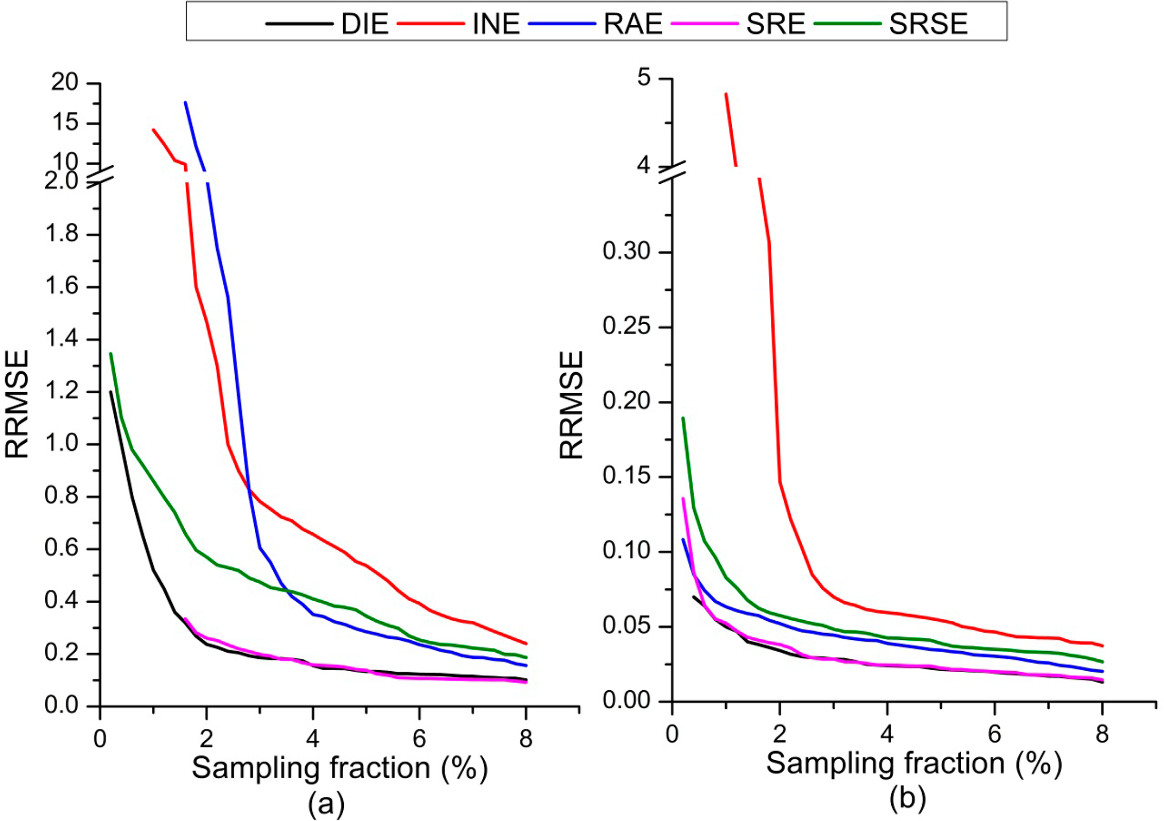
Figure 6 presents the RRMSE in various sampling fractions, which can be calculated by the sample size. As the sampling fraction increases, the RRMSE of the regression group decreases rapidly and becomes stable first. The fewest number of samples required to achieve the same precision of estimation, such as RRMSE = 0.2, for SRE, RAE, DIE, INE, and SRSE was about 375, 400, 625, 875, and 1400, respectively. Thus, SRE requires the fewest samples and is more effective. In addition, it is apparent that increasing the sample size can relieve the precision risk of estimation; we recommend further study to determine whether our results can give a more quantitative predictor. It is worth noting that the curve of SRE began at the 0.02% sampling fraction because of the failure of providing the estimation with the sampling fraction at less than 0.02%.
4.2. Results of Case Study Using Actual Remote Sensing Data
The case study using actual satellite imageries is a realization of operational estimation to verify the results of the simulated experiment described previously. The overall classification accuracies from HJ-1 images in TZ and SY were 50% and 71%, respectively. Comparison results in this study were roughly in agreement with the simulated experiment. The performance of INE was inferior and was even worse than that of SRSE (in TZ). SRE had the best estimations in terms of the evaluation criteria described in Section 3.
We also analyzed the precision of estimation for each land cover class. Figure 7 shows the RRMSE of area estimations of water and built-up land, accounting for 0.94% and 28.39% in SY, respectively. From the figure, it is apparent that SRE can provide a more reliable estimate than the other estimators as long as this relationship is strong and regardless of whether the area of the estimated land cover class is minor or dominant. We also found that, several curves, like INE, SRE, did not begin at the beginning of the sampling fraction range because of the failure of estimation when sampling units are rare.
Because of the distinct spectrum signature, misclassification between water and other land cover classes is rare in auxiliary data (classification from HJ-1 images). By contrast, built-up and bare lands are likely to be misclassified with each other. These errors are distributed complexly, owing to the fragmented pattern of bare land. In the error simulation of internal regions, the class of pixels that is misclassified is assigned randomly, and the spectrum separable properties of land cover/use classes and spatial correlation of classification errors were not revealed in our simulation process; the results for SRE in the simulated experiment are still reliable in this case study. The results also indicate that if the sample size is too small, SRE might be not credible for providing an estimate.
5. Conclusions
Through simulation experiments and practical application, the performance of the confusion matrix calibration estimators, the ratio estimator and the simple regression estimator to various auxiliary data accuracies were studied. The results suggest that the confusion matrix calibration estimators, ratio estimators, and simple regressions can provide more accurate and stable estimates than an SRSE. In addition, high-quality classification data played a positive role in estimation and the confusion matrix inverse estimators were more sensitive to classification accuracy, such as in a simulated experiment. For example, the AD of a confusion matrix calibration inverse estimator decreased by about 0.195 with the increasing overall accuracy of classification; otherwise, the variation of the other three model-assisted estimators was 0.102. Further, a simple regression estimator was slightly superior to the confusion matrix calibration estimator and required fewer sample units under acceptable classification accuracy levels (70%–90%). Moreover, the precision of estimation derived from confusion matrix calibration depends on how well the confusion matrix describes the error in each class. Therefore, improving the description of classification error, for example, by optimizing the distribution of the sample used for constructing the confusion matrix, could be a feasible way to advance the performances of confusion matrix calibration estimators.
The SRE’s performance largely depends on the relationship between auxiliary data and the reference. Low-quality auxiliary data leads to the risk of an unreliable correlation. In some specific situations, we prefer the confusion matrix calibration estimators because they involve less calculation and offer the convenience of achieving accurate assessments and area estimations simultaneously. However, some sacrifice such as sample size may be required. The results reported in this study provide insight into the impact of auxiliary data accuracy, or classification accuracy in this study, on the performance of model-assisted estimators and the selection of area estimation methods, considering the balance of accuracy and simplicity in operational use. Nonetheless, we assumed a simple random sampling scheme in this study, if other sampling designs were used, the results could be different.
Acknowledgments
This study is supported by Major Project of High Resolution Earth Observation System.
Author Contributions
Yaozhong Pan and Yizhan Li conceived and designed the experiments, Yizhan Li and Jianyu Gu worked the simulation procedure, case studies and analyzed the result. Together with Xiufang Zhu, Anzhou Zhao and Xianfeng Liu, they provided the figures and illustrations. Yizhan Li and Xiufang Zhu wrote this paper with Yaozhong Pan’s valuable suggestion.
Conflicts of Interest
The authors declare no conflict of interest.
References
- Lewis, H.G.; Brown, M. A generalized confusion matrix for assessing area estimates from remotely sensed data. Int. J. Remote Sens 2001, 22, 3223–3235. [Google Scholar]
- Gallego, F.J. Remote sensing and land cover area estimation. Int. J. Remote Sens 2004, 25, 3019–3047. [Google Scholar]
- Gallego, F.J.; Bamps, C. Using corine land cover and the point survey lucas for area estimation. Int. J. Appl. Earth Observ. Geoinf 2008, 10, 467–475. [Google Scholar]
- Broich, M.; Stehman, S.V.; Hansen, M.C.; Potapov, P.; Shimabukuro, Y.E. A comparison of sampling designs for estimating deforestation from Landsat imagery: A case study of the Brazilian legal Amazon. Remote Sens. Environ 2009, 113, 2448–2454. [Google Scholar]
- Stehman, S.V. Model-assisted estimation as a unifying framework for estimating the area of land cover and land-cover change from remote sensing. Remote Sens. Environ 2009, 113, 2455–2462. [Google Scholar]
- Pan, Y.Z.; Li, L.; Zhang, J.S.; Liang, S.L.; Zhu, X.F.; Sulla-Menashe, D. Winter wheat area estimation from MODIS-EVI time series data using the crop proportion phenology index. Remote Sens. Environ 2012, 119, 232–242. [Google Scholar]
- Benedetti, R.; Bee, M.; Espa, G.; Piersimoni, G. Part III: GIS and remote sensing. In Agricultural Survey Method; Wiley: New York, NY, USA, 2010; pp. 149–229. [Google Scholar]
- McRoberts, R.E. Probability- and model-based approaches to inference for proportion forest using satellite imagery as ancillary data. Remote Sens. Environ 2010, 114, 1017–1025. [Google Scholar]
- McRoberts, R.E. A model-based approach to estimating forest area. Remote Sens. Environ 2006, 103, 56–66. [Google Scholar]
- Sarndal, C.E.; Swensson, B.; Wretman, J. Model-Assisted Survey Sampling; Springer-Verlag: New York, NY, USA, 1992. [Google Scholar]
- Graubard, B.I.; Korn, E.L. Inference for superpopulation parameters using sample surveys. Stat. Sci 2002, 17, 73–96. [Google Scholar]
- Lohr, S.L. Sampling Design and Analysis, 2nd ed.; Book/Cole: Boston, MA, USA, 2010. [Google Scholar]
- Campbell, J.B. Introduction to Remote Sensing, 2nd ed; Taylor and Francis: London, UK, 1996. [Google Scholar]
- Bauer, M.E.; Hixson, M.M.; Davis, B.J. Area estimation of crops by digital analysis of Landsat data. Photogramm. Eng. Remote Sens 1978, 44, 1033–1043. [Google Scholar]
- Card, D.H. Using known map category marginal frequencies to improve estimates of thematic map accuracy. Photogramm. Eng. Remote Sens 1982, 48, 431–439. [Google Scholar]
- Czaplewski, R.L.; Catts, G.P. Calibration of remotely sensed proportion or area estimates for misclassification error. Remote Sens. Environ 1992, 39, 29–43. [Google Scholar]
- Becker-Reshef, I.; Vermote, E.; Lindeman, M.; Justice, C. A generalized regression-based model for forecasting winter wheat yields in Kansas and Ukraine using MODIS data. Remote Sens. Environ 2010, 114, 1312–1323. [Google Scholar]
- Haack, B.; Rafter, A. Regression estimation techniques with remote sensing: A review and case study. Geocarto Int 2010, 25, 71–82. [Google Scholar]
- Brun, C.; Delince, J.; Leo, O.; Porchier, J.C. Utilisation pilote de l’enquete ter-uti dans les procedures de statistiques agricoles par teledetection. Proceedings of the Conference on Application of Remote Sensing to Agriculture Statistics, Belgirate, Lake Maggiore, Italy, 26–27 November 1992; pp. 43–57.
- Stehman, S.V. Estimating area from an accuracy assessment error matrix. Remote Sens. Environ 2013, 132, 202–211. [Google Scholar]
- McRoberts, R.E. Satellite image-based maps: Scientific inference or pretty pictures? Remote Sens. Environ 2011, 115, 715–724. [Google Scholar]
- McRoberts, R.E. Estimating forest attribute parameters for small areas using nearest neighbors techniques. For. Ecol. Manag 2012, 272, 3–12. [Google Scholar]
- McRoberts, R.E.; Gobakken, T.; Næsset, E. Post-stratified estimation of forest area and growing stock volume using LiDAR-based stratifications. Remote Sens. Environ 2012, 125, 157–166. [Google Scholar]
- McRoberts, R.E.; Walters, B.F. Statistical inference for remote sensing-based estimates of net deforestation. Remote Sens. Environ 2012, 124, 394–401. [Google Scholar]
- McRoberts, R.E.; Næsset, E.; Gobakken, T. Inference for LiDAR-assisted estimation of forest growing stock volume. Remote Sens. Environ 2013, 128, 268–275. [Google Scholar]
- Vibrans, A.C.; McRoberts, R.E.; Moser, P.; Nicoletti, A.L. Using satellite image-based maps and ground inventory data to estimate the area of the remaining Atlantic forest in the Brazilian state of Santa Catarina. Remote Sens. Environ 2013, 130, 87–95. [Google Scholar]
- Domke, G.M.; Woodall, C.W.; Walters, B.F.; McRoberts, R.E.; Hatfield, M.A. Strategies to compensate for the effects of nonresponse on forest carbon baseline estimates from the national forest inventory of the United States. For. Ecol. Manag 2014, 315, 112–120. [Google Scholar]
- Foody, G.M. Assessing the accuracy of land cover change with imperfect ground reference data. Remote Sens. Environ 2010, 114, 2271–2285. [Google Scholar]
- Foody, G.M. Ground reference data error and the mis-estimation of the area of land cover change as a function of its abundance. Remote Sens. Lett 2013, 4, 783–792. [Google Scholar]
- Olofsson, P.; Foody, G.M.; Stehman, S.V.; Woodcock, C.E. Making better use of accuracy data in land change studies: Estimating accuracy and area and quantifying uncertainty using stratified estimation. Remote Sens. Environ 2013, 129, 122–131. [Google Scholar]
- Foody, G.M. Status of land cover classification accuracy assessment. Remote Sens. Environ 2002, 80, 185–201. [Google Scholar]
- Xiao, J.F.; Moody, A. A comparison of methods for estimating fractional green vegetation cover within a desert-to-upland transition zone in central new Mexico, USA. Remote Sens. Environ 2005, 98, 237–250. [Google Scholar]
- Wright, G.G.; Morrice, J.G. Landsat tm spectral information to enhance the land cover of Scotland 1988 dataset. Int. J. Remote Sens 1997, 18, 3811–3834. [Google Scholar]
- Wu, B.; Li, Q. Crop acreage estimation using two individual sampling frameworks with stratification. J. Remote Sens 2004, 8, 551–569. [Google Scholar]
- Jia, B.; Zhu, W.; Pan, Y.; Song, G.; Hu, T. Sensitivity analysis of pre-classification accuracy based on remote sensing. J. Remote Sens 2008, 12, 972–979. [Google Scholar]
- Carfagna, E.; Gallego, F.J. Using remote sensing for agricultural statistics. Int. Stat. Rev 2005, 73, 389–404. [Google Scholar]
- Loveland, T.R.; Zhu, Z.; Ohlen, D.O.; Brown, J.F.; Redd, B.C.; Yang, L. An analysis of the IGBP global land-cover characterization process. Photogramm. Eng. Remote Sens 1999, 65, 1021–1032. [Google Scholar]
- Smith, J.H.; Stehman, S.V.; Wickham, J.D.; Yang, L. Effects of landscape characteristics on land-cover class accuracy. Remote Sens. Environ 2003, 84, 342–349. [Google Scholar]
- Stehman, S.V.; Wickham, J.D. Pixels, blocks of pixels, and polygons: Choosing a spatial unit for thematic accuracy assessment. Remote Sens. Environ 2011, 115, 3044–3055. [Google Scholar]
- Nicholas, T.L. Small area estimation with spatial similarity. Comput. Stat. Data Anal 2010, 54, 1151–1166. [Google Scholar]
- Puertas, O.L.; Brenning, A.; Meza, F.J. Balancing misclassification errors of land cover classification maps using support vector machines and Landsat imagery in the maipo river basin (central Chile, 1975–2010). Remote Sens. Environ 2013, 137, 112–123. [Google Scholar]
- Todd, W.J.; Gehring, D.G.; Hamman, J.F. Landsat wildland mapping accuracy. Photogramm. Eng. Remote Sens 1980, 46, 509–520. [Google Scholar]
- Edwards, T.C., Jr.; Moisen, G.G.; Cutler, D.R. Assessing map accuracy in a remotely sensed, ecoregion-scale cover map. Remote Sens. Environ 1998, 63, 73–83. [Google Scholar]
- Ene, L.T.; Næsset, E.; Gobakken, T.; Gregoire, T.G.; Ståhl, G.; Holm, S. A simulation approach for accuracy assessment of two-phase post-stratified estimation in large-area lidar biomass surveys. Remote Sens. Environ 2013, 133, 210–224. [Google Scholar]
- Chen, J.; Zhu, X.; Imura, H.; Chen, X. Consistency of accuracy assessment indices for soft classification: Simulation analysis. ISPRS J. Photogramm. Remote Sens 2010, 65, 156–164. [Google Scholar]
- Pontius, R.G.; Cheuk, M.L. A generalized cross-tabulation matrix to compare soft-classified maps at multiple resolutions. Int. J. Geograph. Inf. Sci 2006, 20, 1–30. [Google Scholar]
- Okujeni, A.; van der Linden, S.; Tits, L.; Somers, B.; Hostert, P. Support vector regression and synthetically mixed training data for quantifying urban land cover. Remote Sens. Environ 2013, 137, 184–197. [Google Scholar]
- Chen, D.; Wei, H. The effect of spatial autocorrelation and class proportion on the accuracy measures from different sampling designs. ISPRS J. Photogramm. Remote Sens 2009, 64, 140–150. [Google Scholar]


| Classification | ||||||
|---|---|---|---|---|---|---|
| Class 1 | Class 2 | … | Class k | Row Total | ||
| Reference | Class 1 | n11 | n12 | … | n1k | r1 |
| Class 2 | n21 | n22 | … | n2k | r2 | |
| … | … | … | … | … | … | |
| Class k | nk1 | nk2 | … | nkk | rk | |
| Column total | c1 | c2 | … | ck | n | |
| Omission errorclass i = (ri − nii)/ri = 1 − producer’s accuracy | ||||||
| Comission errorclass i = (ci − nii)/ci = 1 − user’s accuracy | ||||||
© 2014 by the authors; licensee MDPI, Basel, Switzerland This article is an open access article distributed under the terms and conditions of the Creative Commons Attribution license (http://creativecommons.org/licenses/by/3.0/).
Share and Cite
Li, Y.; Zhu, X.; Pan, Y.; Gu, J.; Zhao, A.; Liu, X. A Comparison of Model-Assisted Estimators to Infer Land Cover/Use Class Area Using Satellite Imagery. Remote Sens. 2014, 6, 8904-8922. https://doi.org/10.3390/rs6098904
Li Y, Zhu X, Pan Y, Gu J, Zhao A, Liu X. A Comparison of Model-Assisted Estimators to Infer Land Cover/Use Class Area Using Satellite Imagery. Remote Sensing. 2014; 6(9):8904-8922. https://doi.org/10.3390/rs6098904
Chicago/Turabian StyleLi, Yizhan, Xiufang Zhu, Yaozhong Pan, Jianyu Gu, Anzhou Zhao, and Xianfeng Liu. 2014. "A Comparison of Model-Assisted Estimators to Infer Land Cover/Use Class Area Using Satellite Imagery" Remote Sensing 6, no. 9: 8904-8922. https://doi.org/10.3390/rs6098904
APA StyleLi, Y., Zhu, X., Pan, Y., Gu, J., Zhao, A., & Liu, X. (2014). A Comparison of Model-Assisted Estimators to Infer Land Cover/Use Class Area Using Satellite Imagery. Remote Sensing, 6(9), 8904-8922. https://doi.org/10.3390/rs6098904