Automatic Vehicle Extraction from Airborne LiDAR Data Using an Object-Based Point Cloud Analysis Method

Abstract
: Automatic vehicle extraction from an airborne laser scanning (ALS) point cloud is very useful for many applications, such as digital elevation model generation and 3D building reconstruction. In this article, an object-based point cloud analysis (OBPCA) method is proposed for vehicle extraction from an ALS point cloud. First, a segmentation-based progressive TIN (triangular irregular network) densification is employed to detect the ground points, and the potential vehicle points are detected based on the normalized heights of the non-ground points. Second, 3D connected component analysis is performed to group the potential vehicle points into segments. At last, vehicle segments are detected based on three features, including area, rectangularity and elongatedness. Experiments suggest that the proposed method is capable of achieving higher accuracy than the exiting mean-shift-based method for vehicle extraction from an ALS point cloud. Moreover, the larger the point density is, the higher the achieved accuracy is.
1. Introduction
Currently, the airborne laser scanning (ALS, also termed as airborne LiDAR) technique presents a promising alternative to traditional airborne photogrammetry in the generation of digital elevation models (DEMs) [1], reconstruction of 3D building models [2,3], parameter estimation of forests [4,5], urban land cover classification [6], etc. Generally, ALS point cloud filtering is performed as a first step. Because the raw point cloud consists of both the object points and ground points, only the ground points are needed to generate the DEM and normalize the heights of other various types of objects. So far, many ground filtering methods have been proposed to separate the ground points from object points, and most of them are reviewed in [7,8]. Among them, hierarchical linear interpolation [9], progressive TIN (triangular irregular network) densification (PTD) [10], the slope-based method [11] and the morphology-based method [12] are more popular than others.
Meanwhile, vehicle extraction is frequently employed as a part of digital surface model (DSM) generation, as vehicles have to be removed before generating the DSM. Moreover, vehicle extraction is also more frequently used as a part of DTM generation, as the vehicle is a type of man-made object that requires specific filtering. In ALS point cloud filtering, it is hard to separate vehicle points from ground points [13], because vehicle points are very close to the ground surface and they are subject to be regarded as ground points. Yao et al. [14] even classified vehicle points as ground in the filtering stage. Lin and Zhang [13] proposed an object-based point cloud filtering method that works well for vehicle removal. However, vehicle extraction from ALS point cloud data is still a challenging problem due to the variety of vehicle types and the scene complexity.
More and more attention has been paid to vehicle extraction from ALS data [15]. Machine learning is widely employed to extract the vehicle from the ALS data. In [16], after an adaptive mean shift segmentation for extracting local distinct structures, an object-based classification using a binary support vector machine (SVM) is applied to discriminate vehicle points. Moreover, the AdaBoost algorithm [17] and the marked point process model [18] are employed, respectively.
The challenging task is to detect vehicles from the entire point cloud. An obvious idea is using context knowledge for limiting the search space, which can be derived from road databases [19], and then, a significant feature of the vehicle is that it has a certain distribution above the ground. Thus, the determination of measurements belonging to the ground (termed as filtering) is of fundamental interest. Then, based on the elevation data, a representation of vehicles by parameters, such as the size of the footprint and average height values, can be used. Moreover, vehicles can be distinguished from other objects based on their 3D shapes. A simple idea is described by Paska [20] to exploit the 3D profile. First, a bounding box is fitted to the footprint, and the vertical profile of the vehicle is divided into four height sections. Different from the above methods, a new context-based method is proposed by Yao and Stilla [14]. They first classify the vehicles as the ground, and an extended-maxima transform is used to obtain candidate regions. Two thresholds are applied to the amount of pixels and eccentricity of these regions. Finally, the determination of single vehicles is solved by a marker-controlled watershed transformation.
In a word, the context-based approaches are becoming more and more popular in vehicle extraction from the ALS data. However, the existing context-based approaches lack the utilization of the object-based point cloud analysis (OBPCA) method. The OBPCA is introduced for object extraction directly from unorganized point clouds to avoid information loss by rasterization [16], and practices also suggest that the processing of ALS data can be strengthened by OBPCA in which the point clouds are first segmented and then segments rather than individual points are analyzed [21].
In this article, an OBPCA method is proposed to extract vehicles from an ALS point cloud. Particularly, a segmentation-based filter is employed to separate the ground points from the object/non-ground points, the object points whose elevation values within a scope on the ground surface are detected, and then, a 3D connected component analysis (CCA) method is utilized to group the detected object points into segments/clusters. Finally a rule-based classification is performed to extract vehicles based on features of the segments.
The rest of this article is organized as follows. In Section 2, we briefly present our proposed vehicle extraction method. In Section 3, we demonstrate and discuss the experiments and results. Finally, in Section 4, we summarize our studies.
2. Our Vehicle Extraction Method
Our approach is composed of four core steps. First, the ground surface is determined by filtering the LiDAR point cloud using an improved PTD [22]. Subsequently, the object points above a certain height to the ground surface are preserved, and the other points, including the ground points, are removed, which reduces the search space significantly. Third, the object points are clustered by the 3D CCA method [21]. At last, three features of the segments are computed, and the vehicle segments are detected. Details of the steps are listed as follows.
2.1. Filtering
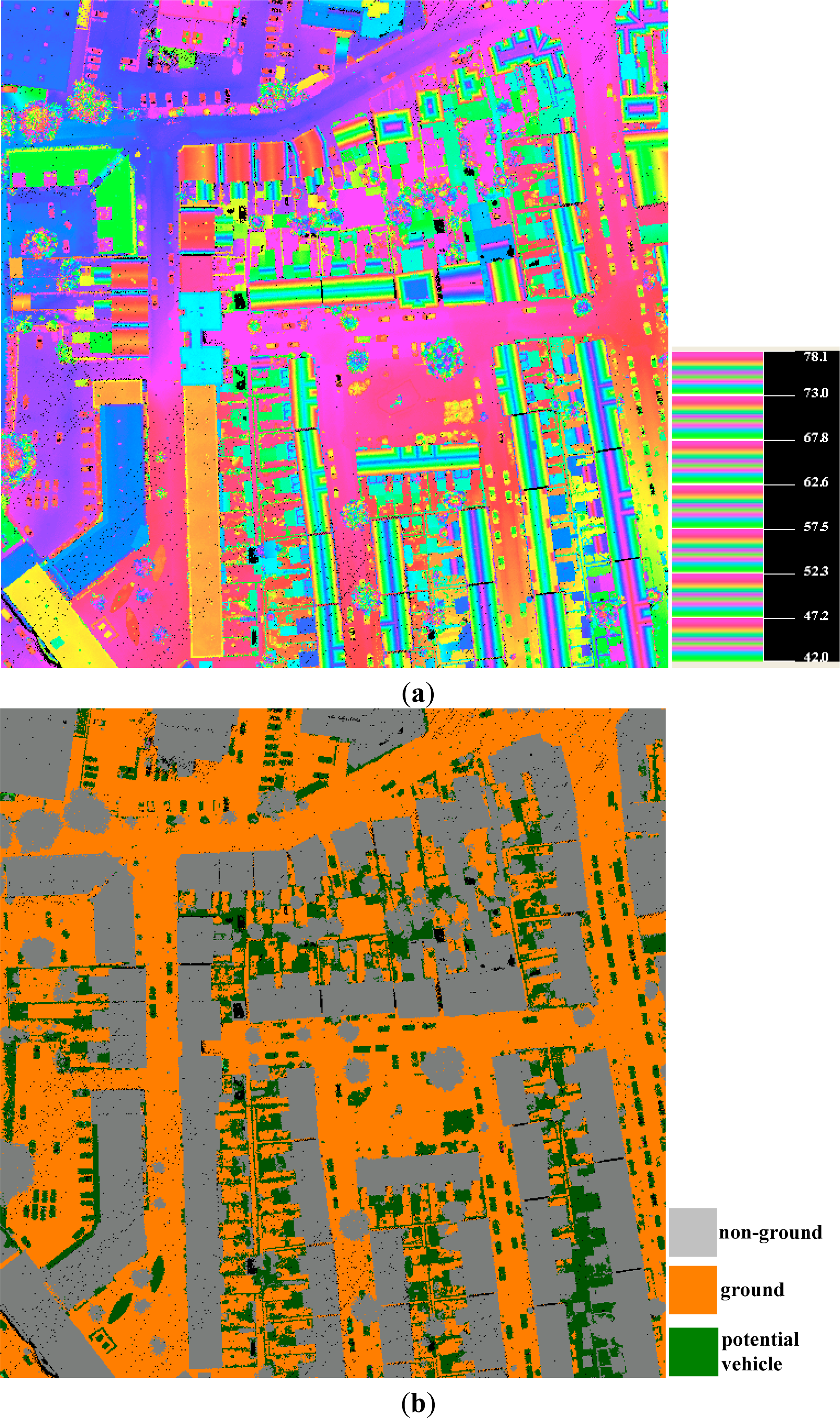
Vehicles in ALS data appear as a bulged object enclosed by surroundings in point cloud data, and the ground surface is always beneath vehicles. This kind of knowledge can help an automatic extraction process. Hence, the separation of ground points from other points is of top priority, and filtering accuracy has a significant influence on the accuracy of vehicle extraction. Lots of filtering methods have been proposed, and an improved PTD is selected [22]. PTD is one of the classic methods for filtering ALS point clouds [10], and it has been widely employed in engineering applications [23,24]. However, it may fail to preserve ground measurements in areas with steep terrain, and it also tends to classify the point belonging to lower parts of the objects as ground [13]. Zhang and Lin [22] improve the PTD using a point cloud segmentation method, namely segmentation using a smoothness constraint (SUSC), and the filtering result of a dataset; see Figure 1.
The classic PTD has two main steps. The first step is selecting seed points and constructing the initial TIN. The second step is an iterative densification of the TIN. The improved method embeds the SUSC between these two steps mentioned above. Specifically, after selecting the lowest points in each grid cell as initial ground seed points, SUSC is employed to expand the set of ground seed points to as many as possible, as this can identify more ground seed points for the subsequent densification of the TIN-based terrain model [22].
Experimental results suggest that, compared with the classic PTD, the improved method is capable of preserving discontinuities of landscapes and reducing the omission errors and total errors. The filtering result of the point cloud in Figure 1a is shown in Figure 1b. Once the ground class is determined, the normalized heights of the non-ground points are to be derived in the next step. The generation of normalized heights is an important step for vehicle extraction from LiDAR data. It sets the whole ground area to the same level and enables the determination of potential vehicle points by comparing normalized height values.
2.2. Detection of Potential Vehicle Points
This step is used to remove the points that can be definitely considered as not vehicles. According to the fact that the vast majority of vehicles is lower than a threshold, h, this step is simply carried out by detecting the points whose normalized heights are lower than h meters from the non-ground points. Specifically, the TIN is constructed using the ground points based on the filtering results, and the TIN is regarded as a representation of the terrain model. For each non-ground point, we find a corresponding triangle of the TIN, and its normalized height is equal to the distance between the non-ground point to the plane where the triangle is placed. If the above derived normalized height is smaller than h, the non-ground point is labeled as a potential vehicle point, as shown in Figure 1b.
2.3. Point Cloud Segmentation
This step will cluster the points into different groups based on characteristics without knowledge of what they really are. The 3D CCA [21] algorithm is a kind of point cloud segmentation, which is employed to solve this problem.
In 3D CCA, fixed distance neighbors (FDNs) are selected to search a local neighborhood of points around each point. The advantage of FDN is that the range of the neighborhood is limited to the immediate local area. The distance metric used is the Euclidean distance. The search for FDN can be optimized using various space partitioning strategies, such as k-d tree. With the help of k-d tree [25], 3D CCA is presented as follows [21]:
- (1)
Specify a distance threshold, dsearch.
- (2)
Set all 3D points to be processed as unlabeled, insert them into a stack and build the k-d tree for the point cloud with the class attribute. The points to be processed probably belong to a specific class.
- (3)
If all of the points have been already labeled, go to Step (7). Otherwise, select the first point without a label in the stack as the current seed, build an empty list of potential seed points and insert the current seed into the list.
- (4)
Select the neighboring points of the current seed using FDN. For points that satisfy having the same class attribute as the current seed, add them to the list of potential seed points.
- (5)
If the number of members in the potential seed point list is larger than one, set the current seed to the next available seed, and go to Step (4). Otherwise, go to Step (6).
- (6)
Give the points in the list a new label, clear the list, and go to Step (3).
- (7)
Finish the task of labeling.
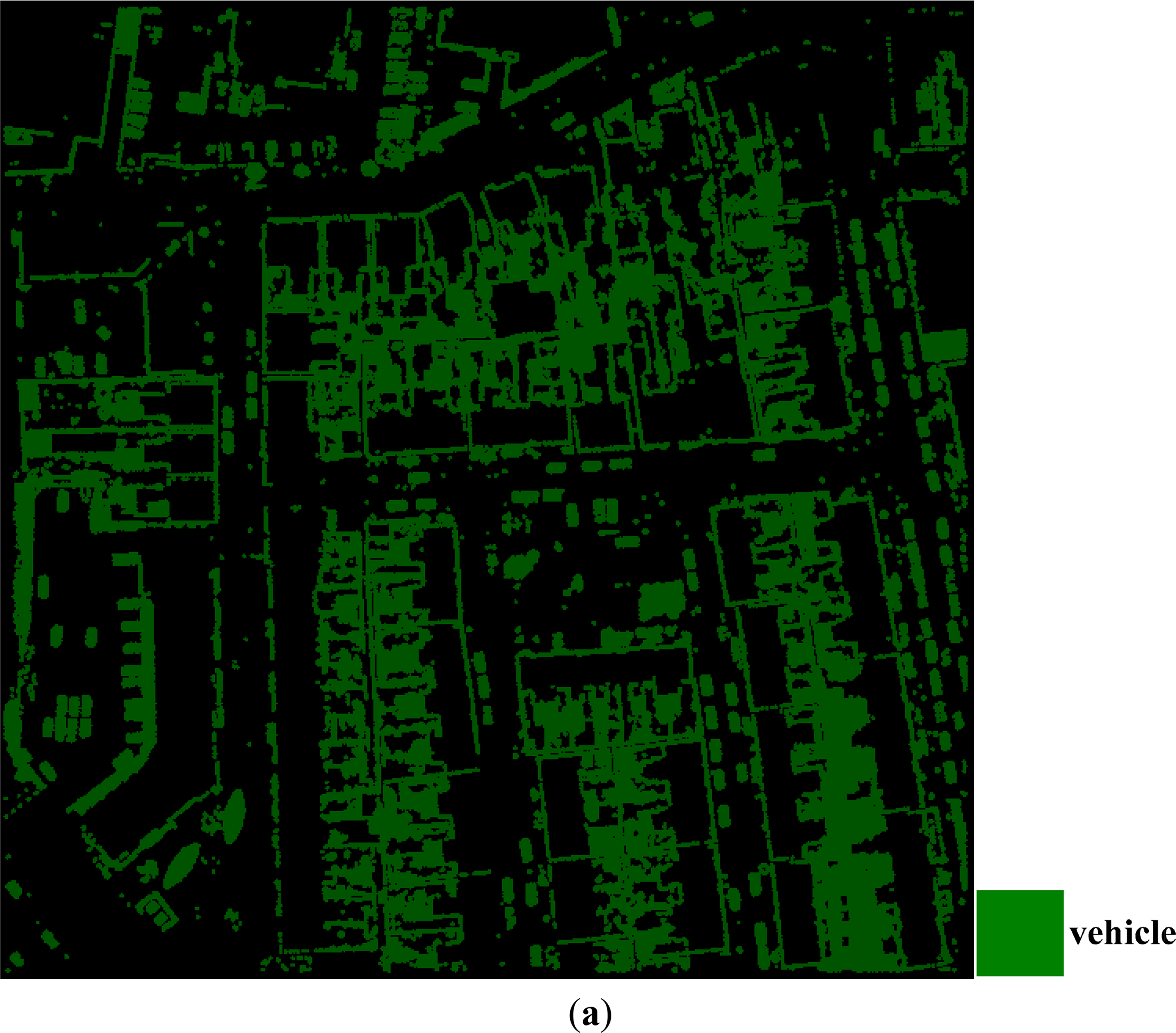
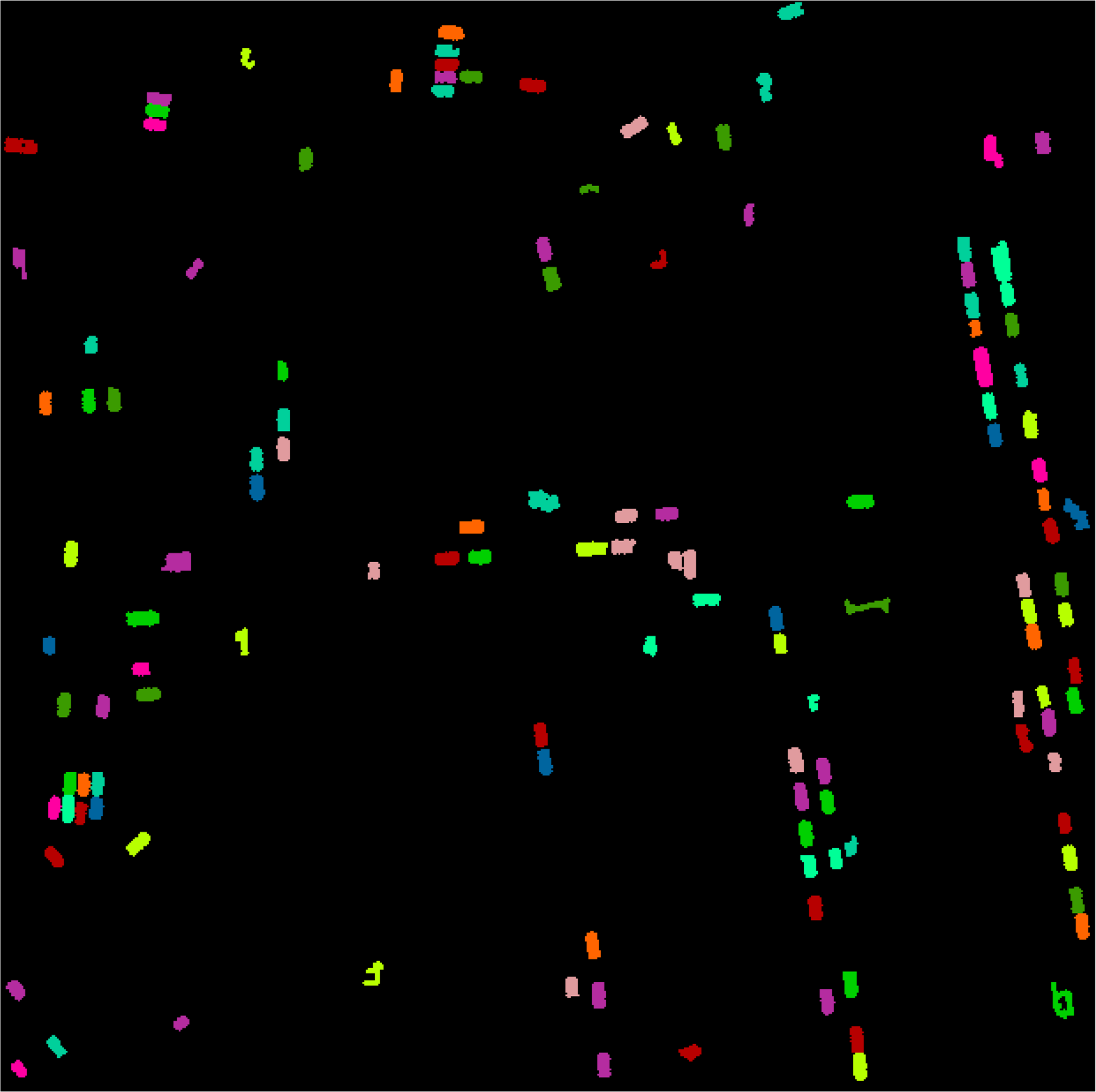
The framework of 3D CCA refers to Figure 2. In this method, the key parameter is the 3D distance threshold, dsearch. The vehicle points in the point cloud of Figure 1c are displayed in Figure 3a, and the corresponding result of 3D CCA is displayed in Figure 3b. Figure 3b shows that, after 3D CCA, the vehicle points are clustered, and the points belonging to the same vehicle may be grouped into the same segment. However, oversegmentation or undersegmentation is still a problem for the above point cloud segmentation if dsearch is not good enough or the scene is too complex, which is inevitable in our proposed method.
2.4. Object-Based Vehicle Extraction
Vehicle extraction is performed based on three features of segments, including area s, rectangularity r, elongatedness e; and they will be defined as follows.
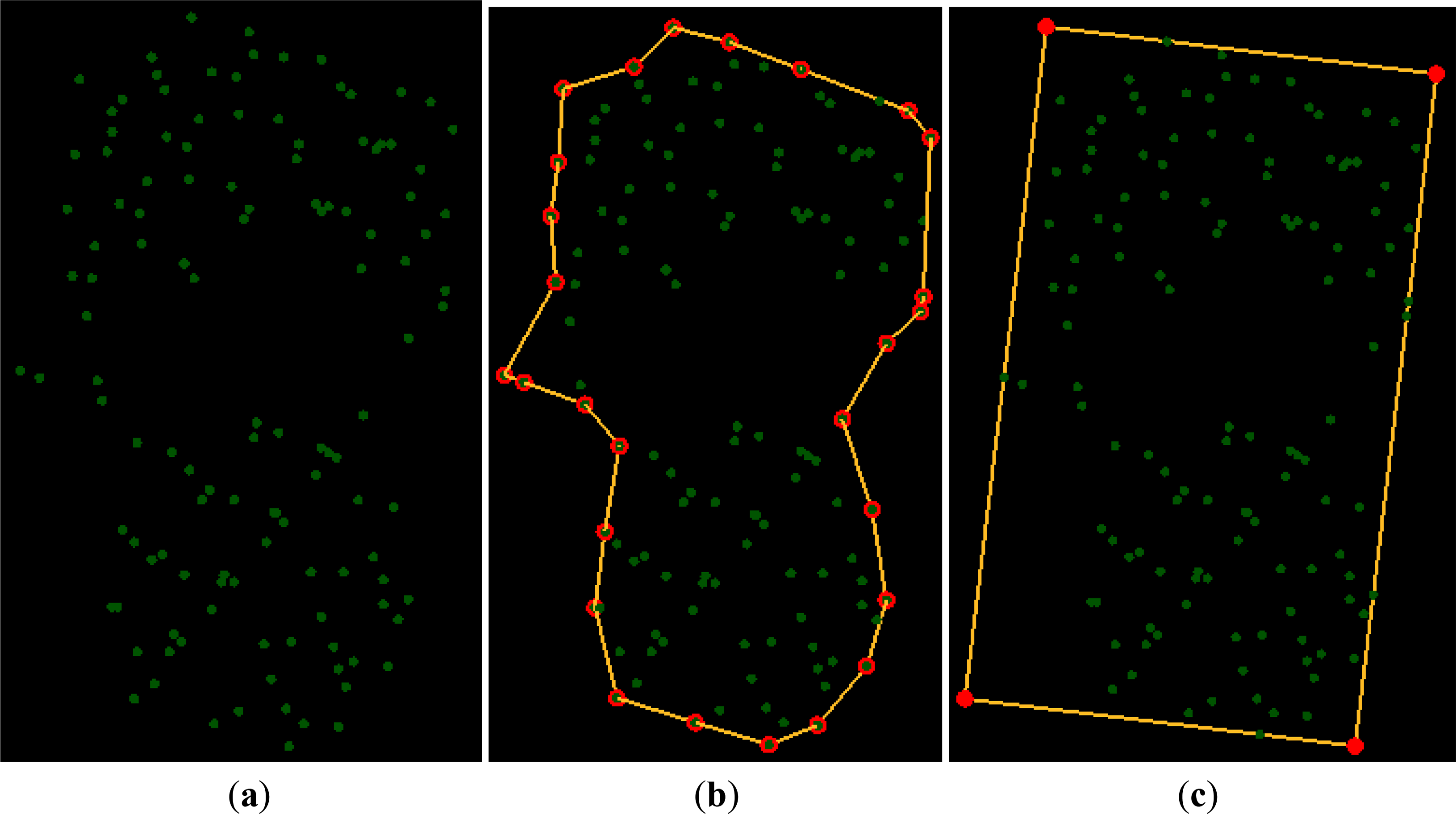
The previous step will derive segments with several 2D geometric properties, including boundary/contour (see Figure 4b), area, perimeter and minimal oriented bounding box (MOBB) (see Figure 4c). In order to compute the 2D geometric features, the points should be transformed into a 2D space from the 3D space. Thus, this can be done by projecting the points of a segment onto the best-fit plane and rotating the plane to be horizontal [21].
Once the transformation is finished, the following geometric properties can be computed as follows:
Boundary: The boundary that closely encompasses the point cluster could be determined by finding the alpha shape of the points, as shown in Figure 4b.
Area: The covered area of the point cluster can be computed using the above derived boundary.
MOBB: The MOBB is calculated from the concave polygon formed by the above derived boundary.
Rectangularity: This is calculated as the ratio of the segment area and its MOBB area.
Elongatedness: This is calculated as the ratio of the length of the short edge of the MOBB and the length of the long edge of the MOBB.
For more details about how to calculate the above features, refer to Zhang et al. [21]. If the values of the three features of a segment are all within a range of scope, the segment is labeled as a vehicle, as shown in Figure 5. Otherwise, the segment is labeled as non-vehicle. Finally, for the vehicle segments, the MOBB of each vehicle segment is extracted, and each MOBB represents a vehicle, as shown in Figure 6b–d.
3. Experiments and Analysis
3.1. The Testing Data
The experiments are carried out on a dataset with a point density of 40 points/m2, as shown in Figure 1a. The data covers an urban area in Enschede, the Netherlands, with a 200-m length and a 200-m width, and it is acquired by a FLI-MAP 400 sensor from John Chance Land Surveys. The FLI-MAP 400 carries a high precision, rotating scanning laser. The scan frequency is up to 250 kHz, and each recording is up to four measurements. The additional element of oblique angle scanning (both seven degrees forward and seven degrees back from nadir) allows a significant reduction in occlusions/shadow effects, resulting in better vegetation penetration. The employed helicopter can fly at a very low height, which guarantees the high point density of the acquired point cloud. It has unbiased global characteristics to guarantee the impartiality of the experiments. Moreover, the dataset is thinned to approximately 20 points/m2 and 10 points/m2, respectively; the thinned two datasets are also employed to verify our approach’s sensitivity to the average point spacing of the point cloud.
3.2. Experimental Results
For all three datasets, the key parameters of the proposed method are set as follows: 0.0 < h < 2.5, 2.0 < s < 15.0, 0.6 < r < 1.0, 0.25 < e < 0.65. Moreover, dsearch is set to 0.4, 0.5 and 1.0 for the point data with a density of 40 points/m2, 20 points/m2 and 10 points/m2, respectively. Those thresholds of the above parameters are determined by checking their histograms and a try-and-error method.
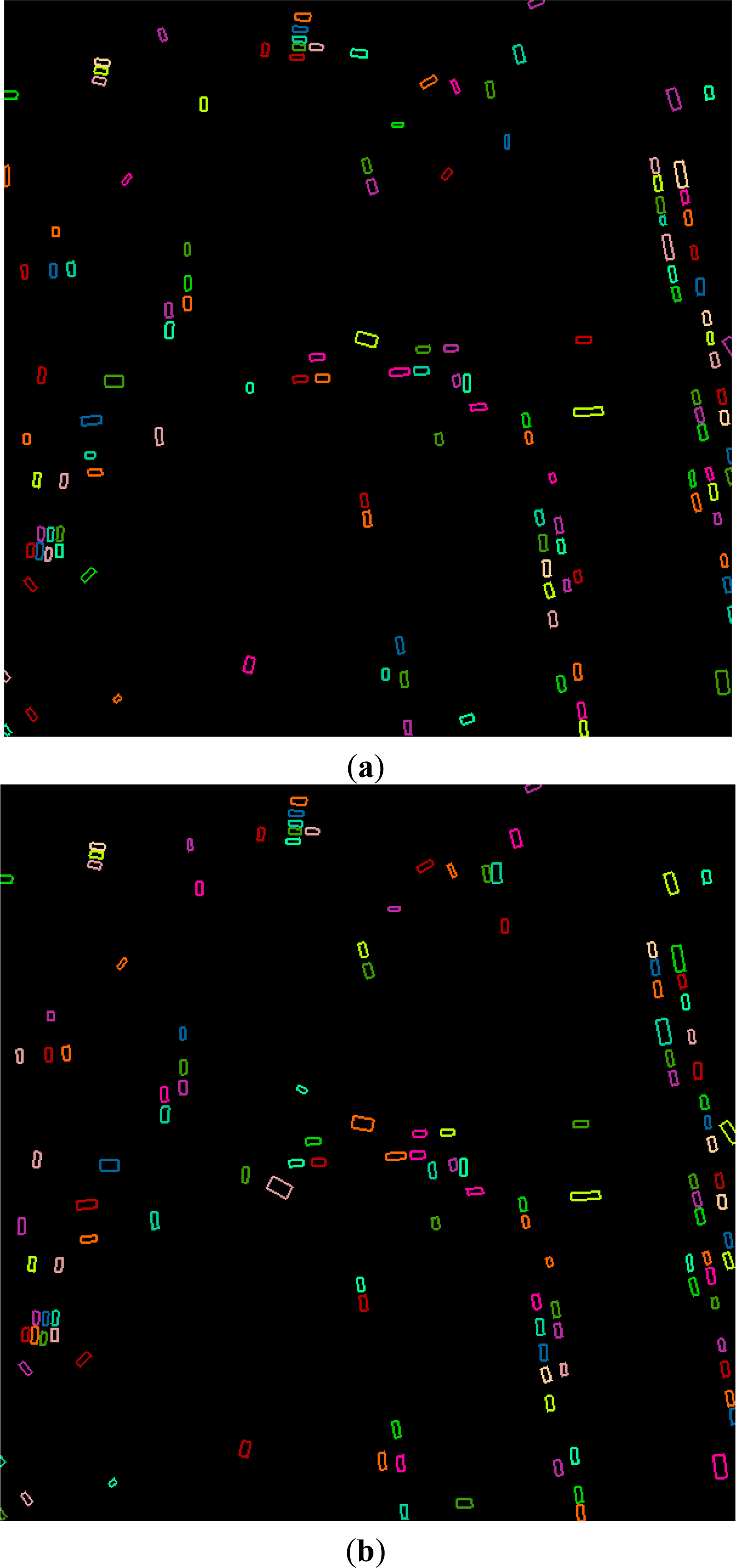
The automatically extracted vehicle from the three datasets by our proposed method is shown in Figure 6b–d. Visual inspection of the results suggest that, when the point density decreases from 40 points/m2 to 10 points/m2, there are more vehicles extracted, but there are more errors. Particularly, there are 129, 131 and 161 vehicles extracted from the dataset with a point density from highest to lowest, respectively. Among them, there are 109, 105 and 103 true vehicles, respectively. Moreover, if the vehicle is very close to low objects or the vehicles are very close to each other, errors may occur, as shown in the ellipse in Figure 6d. Additionally, rectangular objects with the same sizes and heights as the vehicles can be hardly distinguished from vehicles. In short, most of the vehicles are extracted by our proposed method, but there are some errors in the results. Moreover, the proposed method is sensitive to the point density.
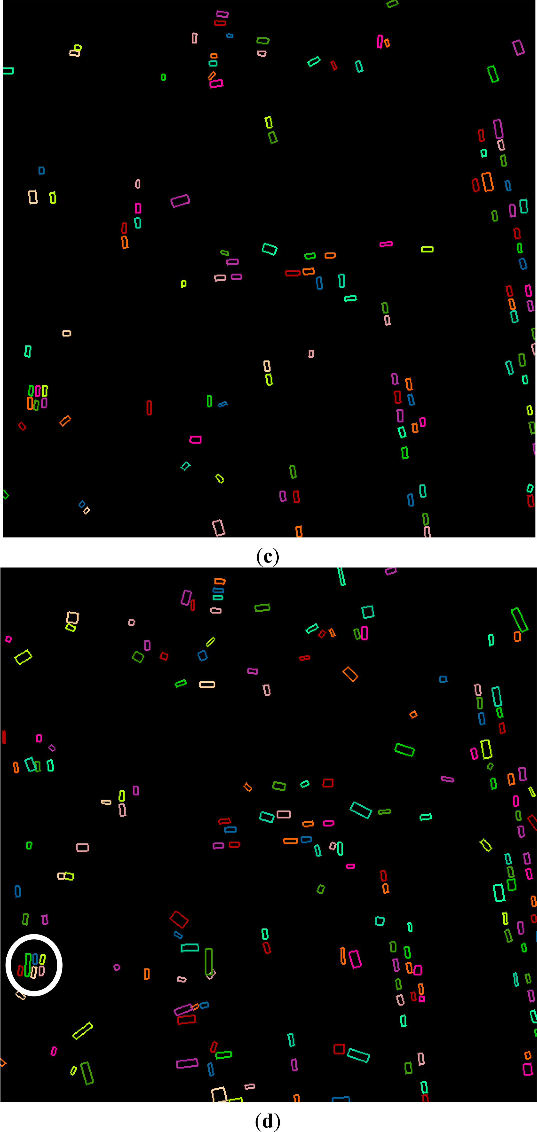
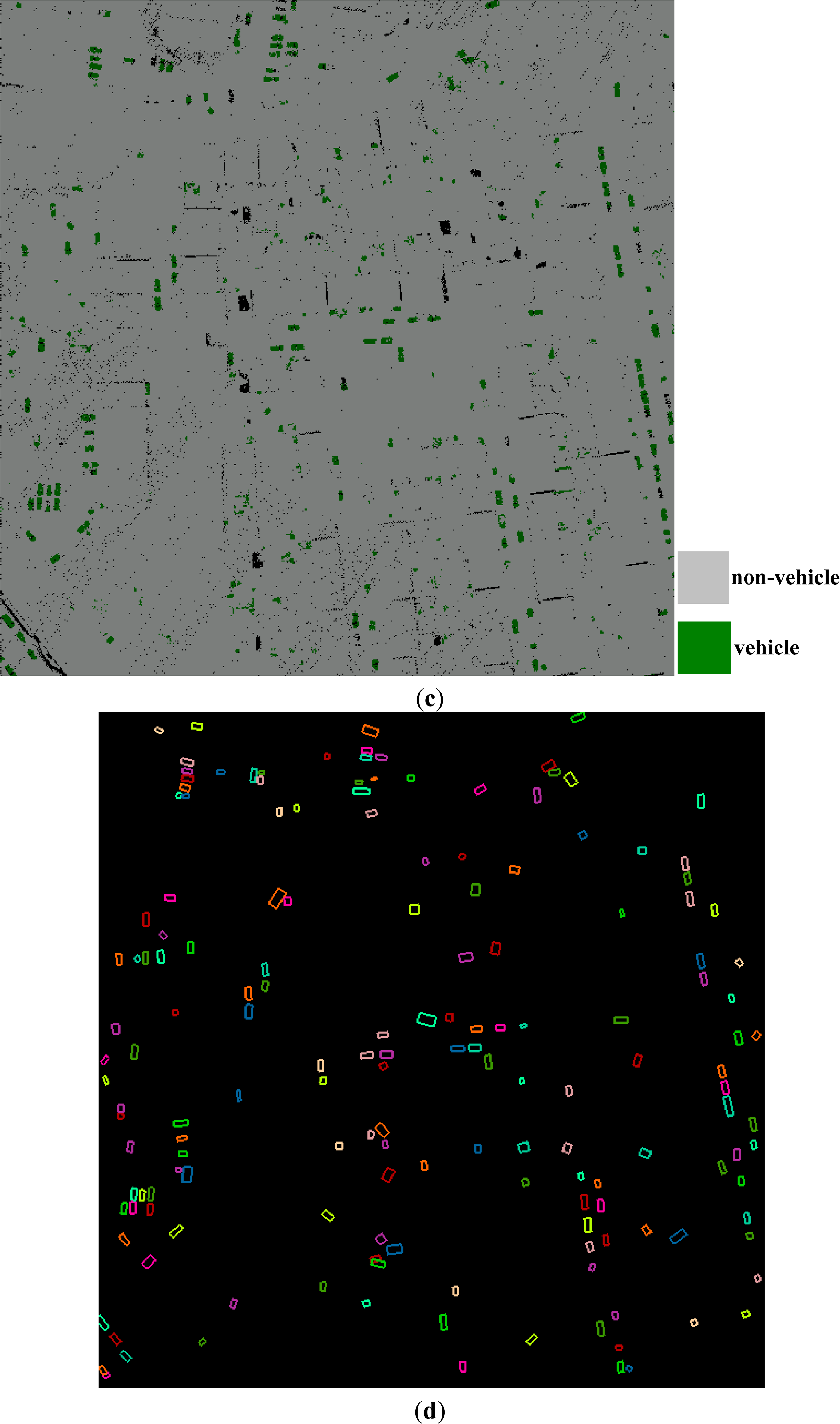
To compare our proposed method with other existing methods, the mean-shift-based vehicle extraction method [16] is also implemented and employed to extract the vehicles from the point cloud with the highest point density. For the implementation of SVM, the software package LIBSVM ( http://www.csie.ntu.edu.tw/~cjlin/libsvm/) by Chang and Lin [26] is adopted; for the implementation of k-d tree, the software package ANN ( http://www.cs.umd.edu/~mount/ANN/) by [27] is adopted; and for the implementation of mean shift, the method in [16,28] is realized. The mean-shift-based segmentation result refers to Figure 7a, and most of the points belonging to one vehicle are segmented into one segment. In the sampling step, two classes of segments, including the vehicle segments and the non-vehicle segments, are selected by a human operator. Note that the sampling progress should be repeated many times based on the SVM-based classification results until there are not many obvious classification errors. In the classification, the features for area, elongatedness, planarity, vertical position and range are employed [16]. As a matter of fact, for the first SVM-based classification, the detected vehicles are quite similar to the ones displayed in Figure 3a based on the initial training samples. Thus, we increase the samples of non-vehicles and the final training samples; see Figure 7b. The final classification result is shown in Figure 7c, and the extracted vehicles refer to Figure 7d. Visual inspection of the result suggests that most vehicles are extracted, while many vehicles are lost, and many non-vehicle objects are also mistaken as vehicles.
3.3. Evaluation
To evaluate the performance of our approach, three measures, including completeness, correctness and quality, are used. Correctness is TP/TP + FP, completeness is TP/TP + FN and quality is TP/TP + FP + FN; where TP is the sum of true positives, FP is the sum of false positives and FN is the sum of false negatives [29]. Moreover, the ground truth data are acquired by manual interpretation of both the original and the filleted point cloud, as shown in Figure 6a. Particularly, there are 136 reference vehicles in the scene.
As far as our method is concerned, the corresponding values of the correctness, completeness and quality of three datasets are shown Table 1. The statistics in Table 1 suggest that values of three measures are affected by the point density. All of the values of three measures are high if the point density is large enough. For example, when the point density is reaching approximately 40 points/m2, the correctness, completeness and quality are approximately 85%, 80% and 70%. Moreover, all of the values of three measures will decrease when the point density is lower. For example, when the point density is decreased to approximately 10 points/m2, the correctness, completeness and quality are approximately 64%, 76% and 53%. Compared with the situation when the point density is reaching approximately 40 points/m2, the correctness, completeness and quality are decreased by approximately 21%, 4% and 17%. Thus, the point density is a very key factor for the extraction of vehicles from the airborne point cloud. In a word, the above statistics suggest that our proposed method performs well if the point density is large enough.
For the mean-shift-based vehicle extraction method [16], the corresponding values of the correctness, completeness and quality of the dataset with a point density of 40 points/m2 are 64.71%, 72.79% and 52.11%. Compared with our proposed method, the correctness, completeness and quality is decreased by approximately 20%, 7% and 18%. The above statistics suggest that our proposed method performs better than the mean-shift-based vehicle extraction method [16] for the employed testing dataset.
3.4. Analysis and Discussion
The above experiments suggest that our proposed OBPCA method is sensitive to point density, and the best extraction result is acquired on the dataset with the highest point density. Table 1 shows that there are 129, 131 and 161 vehicles extracted from the dataset with a point density of 40, 20 and 10 points/m2, respectively. Correspondingly, the correctness is 84.50%, 80.15% and 63.98%, respectively. Table 1 also shows that there are 27, 31 and 33 vehicles being omitted for the corresponding three datasets. This phenomenon suggests that the detailed description of vehicles using more points is helpful to detect the vehicles and separate the vehicles from the others in terms of the state-of-the-art ALS technology. Actually, a good description and representation of any object using points needs enough points from the surface of the object; so does a vehicle. However, the vehicle is a type of smaller object compared with other types of objects, such as building roofs and tree crowns. Thus, a higher point density is needed to describe a vehicle than a building roof when ALS technology is employed. In other words, when the urban scene and the corresponding objects are fixed, more scanned points are needed to describe small objects well, such as vehicles. In our experiments, 40 points/m2 may be high enough to describe the vehicles. On the other hand, if the point density is reduced, there may not be enough points to describe the smaller objects. For example, when the point density of a point cloud is fixed to approximately 10 points/m2, there are fewer points from smaller vehicles than larger objects. In this situation, the point density may be enough for a detailed description of larger objects, but it may not be enough for a detailed description of small objects, such as vehicles. If all of the small objects cannot be well depicted by the corresponding points, some features of small objects are prone to be similar, and thus, they may be misclassified. For example, more vehicles can be extracted from the dataset with a point density of 10 points/m2 than the dataset with the highest point density, as shown in Figure 6b,d and Table 1. Thus, more points are needed for a detailed description of small objects, which means a higher point density. As a result, the higher the point density is, the more detailed the description of the vehicle is. When a vehicle is better depicted, the extraction result can be better achieved.
The above experiments also suggest that the performance of our proposed OBPCA method is better than the mean-shift-based vehicle extraction method [16]. This phenomenon is relevant to the similarity between vehicles and other objects. In urban environments, there are various types of objects, and there are many similar objects to the vehicles if only a few features are considered. As shown in Figure 3b, there are many rectangular objects in the urban point cloud, even if only the objects close to the ground are considered. Thus, it is difficult to accurately recognize the vehicles if only machine learning is employed, as done by the mean-shift-based vehicle extraction method [16]. In the result of the method in [16], there are 35% errors, as shown in Table 1. Moreover, an elaborative selection of the samples is needed for the machine learning method. However, it is hard for a human being to select the optimal samples for complex urban scenes. In our experiments, the final training samples for the mean-shifted method are determined by many rounds of selection, and they are still unsatisfying. Thus, the optimal classification result is hard to obtain using the machine learning method. Different from the method in [16], our proposed OBPCA method makes use of the context and existing knowledge, which decreases the search space, thus increasing the accuracy.
4. Conclusions
This article presents an object-based point cloud analysis method to automatically extract vehicles from an ALS point cloud. The method only relies on the 3D laser point cloud, and it needs no additional data source, such as road databases. The experiments suggest that the proposed approach is able to achieve higher accuracy than the mean-shift-based method if the point cloud is dense enough. The experiments also suggest that the larger the point density is, the better the proposed method performs. However, the proposed method is unable to separate the rectangular objects with similar areas and heights as the vehicles. In the future, enhanced results might be achieved with the aid of the pulse intensity and data fusion strategy, and vehicles under trees may be focused on. Moreover, parallel computing [30] will be adopted to speed up the efficiency.
Acknowledgments
This research was funded by: (1) the General Program sponsored by the National Natural Science Foundations of China (NSFC) under Grant 41371405; (2) the Scientific and Technological Project for National Basic Surveying and Mapping with the title, Research on Theory and Method for Object-oriented Vehicle Extraction from Airborne LiDAR Point Cloud; (3) the Basic Research Fund of Chinese Academy of Surveying and Mapping under Grant 7771413, respectively. Moreover, the Enschede data set is kindly provided by Shi Pu from the Faculty of Geo-Information Science and Earth Observation of the University of Twente.
Author Contributions
All of the authors contributed extensively to the work presented in this paper. Particularly, Jixian Zhang has made the main contribution on writing most of the manuscript. Minyan Duan has written part of the manuscript, and performed the experiments and experimental analysis. Qin Yan has proposed the original idea, supplied the hardware for coding and experiments, and provided the chance for academic exchange. Xiangguo Lin has made the contribution on the programming, and revised the manuscript.
Conflicts of Interest
The authors declare no conflict of interest.
References
- Hu, H.; Ding, Y.; Zhu, Q.; Wu, B.; Lin, H.; Du, Z.; Zhang, Y.; Zhang, Y. An adaptive surface filter for airborne laser scanning point clouds by means of regularization and bending energy. ISPRS J. Photogramm. Remote Sens 2014, 92, 98–111. [Google Scholar]
- Xiong, B.; Oude Elberink, S.; Vosselman, G. A graph edit dictionary for correcting errors in roof topology graphs reconstructed from point clouds. ISPRS J. Photogramm. Remote Sens 2014, 93, 227–242. [Google Scholar]
- Wang, R. 3D building modeling using images and LiDAR: A review. Int. J. Image Data Fusion 2013, 4, 273–292. [Google Scholar]
- Hyyppä, J.; Yu, X.; Hyyppä, H.; Vastaranta, M.; Holopainen, M.; Kukko, A.; Kaartinen, H.; Jaakkola, A.; Vaaja, M.; Koskinen, J.; et al. Advances in forest inventory using airborne laser scanning. Remote Sens 2012, 4, 1190–1207. [Google Scholar]
- Wang, C.; Menenti, M.; Stoll, M.P.; Feola, A.; Belluco, E.; Marani, M. Separation of ground and low vegetation signatures in LiDAR measurements of salt-marsh environments. IEEE Trans. Geosci. Remote Sens 2009, 47, 2014–2023. [Google Scholar]
- Richter, R.; Behrens, M.; Döllner, J. Object class segmentation of massive 3D point clouds of urban areas using point cloud topology. Int. J. Remote. Sens 2013, 34, 8408–8424. [Google Scholar]
- Meng, X.; Currit, N.; Zhao, K. Ground filtering algorithms for airborne LiDAR data: A review of critical issues. Remote Sens 2010, 2, 833–860. [Google Scholar]
- Sithole, G.; Vosselman, G. Experimental comparison of filter algorithms for bare earth extraction from airborne laser scanning point clouds. ISPRS J. Photogramm. Remote Sens 2004, 59, 85–101. [Google Scholar]
- Kraus, K.; Pfeifer, N. Determination of terrain models in wooded areas with airborne laser scanner data. ISPRS J. Photogramm. Remote Sens 1998, 53, 193–203. [Google Scholar]
- Axelsson, P.E. DEM generation from laser scanner data using adaptive TIN models. Int. Arch. Photogramm. Remote Sens 2000, 32, 110–117. [Google Scholar]
- Vosselman, G. Slope based filtering of laser altimetry data. Int. Arch. Photogramm. Remote Sens 2000, 33, 935–942. [Google Scholar]
- Zhang, K.Q.; Chen, S.C.; Whitman, D.; Shyu, M.L.; Yan, J.H.; Zhang, C.C. A progressive morphological filter for removing nonground measurements from airborne LIDAR data. IEEE Trans. Geosci. Remote Sens 2003, 41, 872–882. [Google Scholar]
- Lin, X.; Zhang, J. Segmentation-based filtering of airborne LiDAR point clouds by progressive densification of terrain segments. Remote Sens 2014, 6, 1294–1326. [Google Scholar]
- Yao, W.; Hinz, S.; Stilla, U. Automatic vehicle extraction from airborne LiDAR data of urban areas aided by geodesic morphology. Pattern Recogn. Lett 2010, 31, 1100–1108. [Google Scholar]
- Hinz, S.; Bamler, R.; Stilla, U. Theme issue: “Airborne and spaceborne traffic monitoring”. ISPRS J. Photogramm. Remote Sens 2006, 61, 135–136. [Google Scholar]
- Yao, W.; Stilla, U. Comparison of two methods for vehicle extraction from airborne LiDAR data toward motion analysis. IEEE Geosci. Remote Sens. Lett 2011, 8, 607–611. [Google Scholar]
- Yang, B.; Sharma, P.; Nevatia, R. Vehicle detection from low quality aerial LIDAR data. Proceedings of 2011 IEEE Workshop on Applications of Computer Vision (WACV), Kona, HI, USA, 5–7 January 2011; pp. 541–548.
- Börcs, A.; Benedek, C. A marked point process model for vehicle detection in aerial LIDAR point clouds. ISPRS Ann. Photogramm. Remote Sens. Spat. Inf. Sci. 2012, I-3, 93–98. [Google Scholar]
- Toth, C.; Grejner-Brzezinska, D. Extracting dynamic spatial data from airborne imaging sensors to support traffic flow estimation. ISPRS J. Photogramm. Remote Sens 2006, 61, 137–148. [Google Scholar]
- Paska, E.P. State-of-the-Art Remote Sensing Geospatial Technologies in Support of Transportation Monitoring and Management; Ph.D. Thesis, The Ohio State University, Columbus, OH, USA; 2009. [Google Scholar]
- Zhang, J.X.; Lin, X.G.; Ning, X.G. SVM-based classification of segmented airborne LiDAR point clouds in urban areas. Remote Sens 2013, 5, 3749–3775. [Google Scholar]
- Zhang, J.X.; Lin, X.G. Filtering airborne LiDAR data by embedding smoothness-constrained segmentation in progressive TIN densification. ISPRS J. Photogramm. Remote Sens 2013, 81, 44–59. [Google Scholar]
- Zhu, X.K.; Toutin, T. Land cover classification using airborne LiDAR products in Beauport, Québec, Canada. Int. J. Image Data Fusion 2013, 4, 252–271. [Google Scholar]
- Shen, J.; Liu, J.; Lin, X.; Zhao, R. Object-based classification of airborne light detection and ranging point clouds in human settlements. Sens. Lett 2012, 10, 221–229. [Google Scholar]
- Arya, S.; Mount, D.M.; Netanyahu, N.S.; Silverman, R.; Wu, A.Y. An optimal algorithm for approximate nearest neighbor searching in fixed dimensions. J. ACM 1998, 45, 891–923. [Google Scholar]
- Chang, C.C.; Lin, C.J. LIBSVM: A Library for Support Vector Machines. 2001. Available online: http://www.csie.ntu.edu.tw/~cjlin/libsvm (accessed on 15 March 2010). [Google Scholar]
- ANN: A Library for Approximate Nearest Neighbor Searching. Available online: http://www.cs.umd.edu/~mount/ANN/ (accessed on 15 March 2010).
- Huang, X.; Zhang, L. An adaptive mean-shift analysis approach for object extraction and classification from urban hyperspectral imagery. IEEE Trans. Geosci. Remote Sens 2008, 46, 4173–4185. [Google Scholar]
- Tuermer, S.; Kurz, F.; Reinartz, P.; Stilla, U. Airborne vehicle detection in dense urban areas using HoG features and disparity maps. IEEE J. Sel. Top. Appl. Earth Obs. Remote Sens 2013, 6, 2327–2337. [Google Scholar]
- Kang, X.; Liu, J.; Lin, X. Streaming progressive TIN densification filter for airborne LiDAR point clouds using multi-core architectures. Remote Sens 2014, 6, 7212–7232. [Google Scholar]


| Methods | Point Density (points/m2) | TP | FP | FN | Correctness (%) | Completeness (%) | Quality (%) |
|---|---|---|---|---|---|---|---|
| Our OBPCA method | 40 | 109 | 27 | 20 | 84.50 | 80.15 | 69.87 |
| 20 | 105 | 31 | 26 | 80.15 | 77.21 | 64.81 | |
| 10 | 103 | 33 | 58 | 63.98 | 75.74 | 53.09 | |
| The method in [16] | 40 | 99 | 37 | 54 | 64.71 | 72.79 | 52.11 |
© 2014 by the authors; licensee MDPI, Basel, Switzerland This article is an open access article distributed under the terms and conditions of the Creative Commons Attribution license (http://creativecommons.org/licenses/by/3.0/).
Share and Cite
Zhang, J.; Duan, M.; Yan, Q.; Lin, X. Automatic Vehicle Extraction from Airborne LiDAR Data Using an Object-Based Point Cloud Analysis Method. Remote Sens. 2014, 6, 8405-8423. https://doi.org/10.3390/rs6098405
Zhang J, Duan M, Yan Q, Lin X. Automatic Vehicle Extraction from Airborne LiDAR Data Using an Object-Based Point Cloud Analysis Method. Remote Sensing. 2014; 6(9):8405-8423. https://doi.org/10.3390/rs6098405
Chicago/Turabian StyleZhang, Jixian, Minyan Duan, Qin Yan, and Xiangguo Lin. 2014. "Automatic Vehicle Extraction from Airborne LiDAR Data Using an Object-Based Point Cloud Analysis Method" Remote Sensing 6, no. 9: 8405-8423. https://doi.org/10.3390/rs6098405
APA StyleZhang, J., Duan, M., Yan, Q., & Lin, X. (2014). Automatic Vehicle Extraction from Airborne LiDAR Data Using an Object-Based Point Cloud Analysis Method. Remote Sensing, 6(9), 8405-8423. https://doi.org/10.3390/rs6098405