Article

Potential of X-Band Images from High-Resolution Satellite SAR Sensors to Assess Growth and Yield in Paddy Rice

1
National Institute for Agro-Environmental Sciences, Tsukuba, Ibaraki 305-8604, Japan
2
Aomori-ITC Agricultural Research Institute, Kuroishi 036-0522, Japan
3
Department of Geography, University of South Carolina, Columbia, SC 29208, USA
*
Author to whom correspondence should be addressed.
Remote Sens. 2014, 6(7), 5995-6019; https://doi.org/10.3390/rs6075995
Submission received: 11 April 2014 / Revised: 13 May 2014 / Accepted: 5 June 2014 / Published: 27 June 2014

Abstract

:
The comprehensive relationship of backscattering coefficient (σ0) values from two current X-band SAR sensors (COSMO-SkyMed and TerraSAR-X) with canopy biophysical variables were investigated using the SAR images acquired at VV polarization and shallow incidence angles. The difference and consistency of the two sensors were also examined. The chrono-sequential change of σ0 in rice paddies during the transplanting season revealed that σ0 reached the value of nearby water surfaces a day before transplanting, and increased significantly just after transplanting event (3 dB). Despite a clear systematic shift (6.6 dB) between the two sensors, the differences in σ0 between target surfaces and water surfaces in each image were comparable in both sensors. Accordingly, an image-based approach using the “water-point” was proposed. It would be useful especially when absolute σ0 values are not consistent between sensors and/or images. Among the various canopy variables, the panicle biomass was found to be best correlated with X-band σ0. X-band SAR would be promising for direct assessments of rice grain yields at regional scales from space, whereas it would have limited capability to assess the whole-canopy variables only during the very early growth stages. The results provide a clear insight on the potential capability of X-band SAR sensors for rice monitoring.

1. Introduction

Consistent and efficient observation of crops and agroecosystems is one of the most important applications of remote sensing. Timely assessment of crop conditions (e.g., planted area, growth, productivity, damage) is critical for diagnosis and decision making for precision crop management and food security, especially under recent conditions associated with climate change [14]. The negative impacts of agriculture, such as air and water pollution by N2O, e.g., [5] and NO3, e.g., [6] from farming practices, can be minimized based on geospatial information on actual crop and farmland status, e.g., [7]. Many studies have shown that the synthetic aperture radar (SAR) sensors have great potential for a wide range of agricultural applications due to their superior ability in timely observation of land surfaces, e.g., [813]. The rain or heavy clouds would affect SAR image data, especially in high frequency bands (e.g., Ka, Ku, or X), through the disturbance in signal-propagation and/or the physical changes in land surfaces [14]. However, the certainty of image acquisition at a desired timing as well as the stability of data quality are far superior in SAR than in optical sensors.
Rice (Oryza sativa L.) is the most important staple crop in Asia. Under the cloudy weather conditions in monsoon Asia, SAR sensors are particularly useful for timely monitoring the growth and yield of rice. For classification purposes, SAR images in X and C-bands have already been used operationally for the assessment of rice-cropped areas because the extraction of rice fields is relatively robust due to the specular feature under flooded surface conditions, e.g., [1517]. Similarly, information regarding cropping systems or agricultural management practices in rice growing regions may be obtained successfully from X and C-band SAR observations, e.g., [13,1820].
However, quantitative assessments of ecophysiological or biophysical rice variables using satellite SAR signatures remain uncertain, although they are crucial for various agricultural applications. According to the review by Lopez-Sanchez and Ballester-Berman [11], various experimental studies based on ground-based scatterometers have shown the great potential of microwave remote sensing for the assessment of rice biophysical variables, e.g., [2123]. For example, Inoue et al. [23] reported comprehensive results on the potential of various frequency bands based on a unique dataset of daily backscattering coefficients (σ0) taken in all of the combinations of five frequency bands (Ka, Ku, X, C, L), four polarizations (VV, VH, HV, HH), and four incidence angles (25°, 35°, 45°, 55°) during a full growing period of paddy rice. Despite such potentials, many studies using satellite SAR images have suggested only preliminary relationships between σ0 and rice variables such as plant height, e.g., [16,24,25]. The accuracies reported in such papers seem insufficient for routine/operational applications.
One reason for such uncertainties in crop monitoring applications was the low spatial resolution of SAR images. In general, high spatial resolution (1–5 m) is required for many agricultural applications in Asian countries because of the small size of agricultural fields. SAR technology realized much higher spatial resolutions compared to real aperture radars; however, spatial resolutions in previous generation of sensors (10 m∼) were not enough for such applications and for precise biophysical investigations due to the degradation of resolution by de-speckling processes. Another limitation was the insufficient ground-based data relating to ecophysiological or biophysical status, which could lead to superficial relationships or misinterpretations. From eco-physiological aspects, the reported relationships of SAR signatures with plant variables are sometimes indirect or superficial, which implies the limited applicability. Although some polarimetric parameters such as entropy and alpha derived from multi-polarization images [19,26] may provide additional information on canopy and surface conditions, further investigations have to be based on the detailed biophysical rice measurements to achieve sufficient accuracy and robustness as well as a clear interpretation of the relationships. Moreover, physically-based backscattering models may be useful for the interpretation of measured data, e.g., [8,22,27], but they require significant improvement in structure and parameterization to retrieve biophysical variables with sufficient accuracy. Such investigations would require a more detailed sensitivity analysis based on accurate canopy biophysical measurements.
Therefore, ecophysiological investigations based on high resolution SAR signatures and accurate concurrent measurements of biophysical variables are critical. The spotlight mode of recent high-resolution satellite SAR sensors (e.g., COSMO-SkyMed: CSK, TerraSAR-X: TSX, Radarsat-2) would allow such detailed and robust analyses. For example, a recent study using Radarsat-2 sensor (spotlight mode) elucidated the ability and inability of C-band SAR for rice monitoring, e.g., [13]. However, biophysical or ecophysiological investigations on the potential of X-band SAR for rice monitoring are not sufficient. Recent studies using CSK and TSX have suggested certain relationships with vegetation parameters and soil moisture [2835], but consistent and accurate relationships are not established. In addition, some discrepancies have been recognized between σ0 values from CKS and TSX, e.g., [36,37]. Pettinato et al. [37] suggested that CSK data would be corrected against TSX (Stripmap mode) by adding about 4 dB in Ping Pong mode and about 2.5 dB in Himage mode, respectively. They also suggested that these values may vary with measurement configurations, i.e., mode, orbit, polarization, and incidence angle. Hence, the consistency of σ0 values between sensors has to be elucidated for rice monitoring applications. However, more importantly, the generality of relationships between canopy biophysical variables and σ0 values from different sensors is essential for the combined use, i.e., constellation of different satellite sensors for timely monitoring of agricultural applications. A recent preliminary analysis using CSK suggested that the X-band σ0 at VV polarization at a shallow incidence angle was closely correlated with the weight of rice panicle (ear) [12]. The study also undertook a comprehensive comparison of σ0 with a range of canopy biophysical variables during the maturing stage. However, the generality and consistency of such relationships for different sensors such as TSX are unknown.
Thus, the objectives of this study were to examine the differences and consistency of the two high-resolution X-band SAR sensors (i.e., CSK and TSX) for rice monitoring, investigate the comprehensive relationship of σ0 values from CSK and TSX with canopy biophysical variables, and explore the unique capabilities of the X-band sensors for assessment of rice growth and yield.

2. Materials and Methods
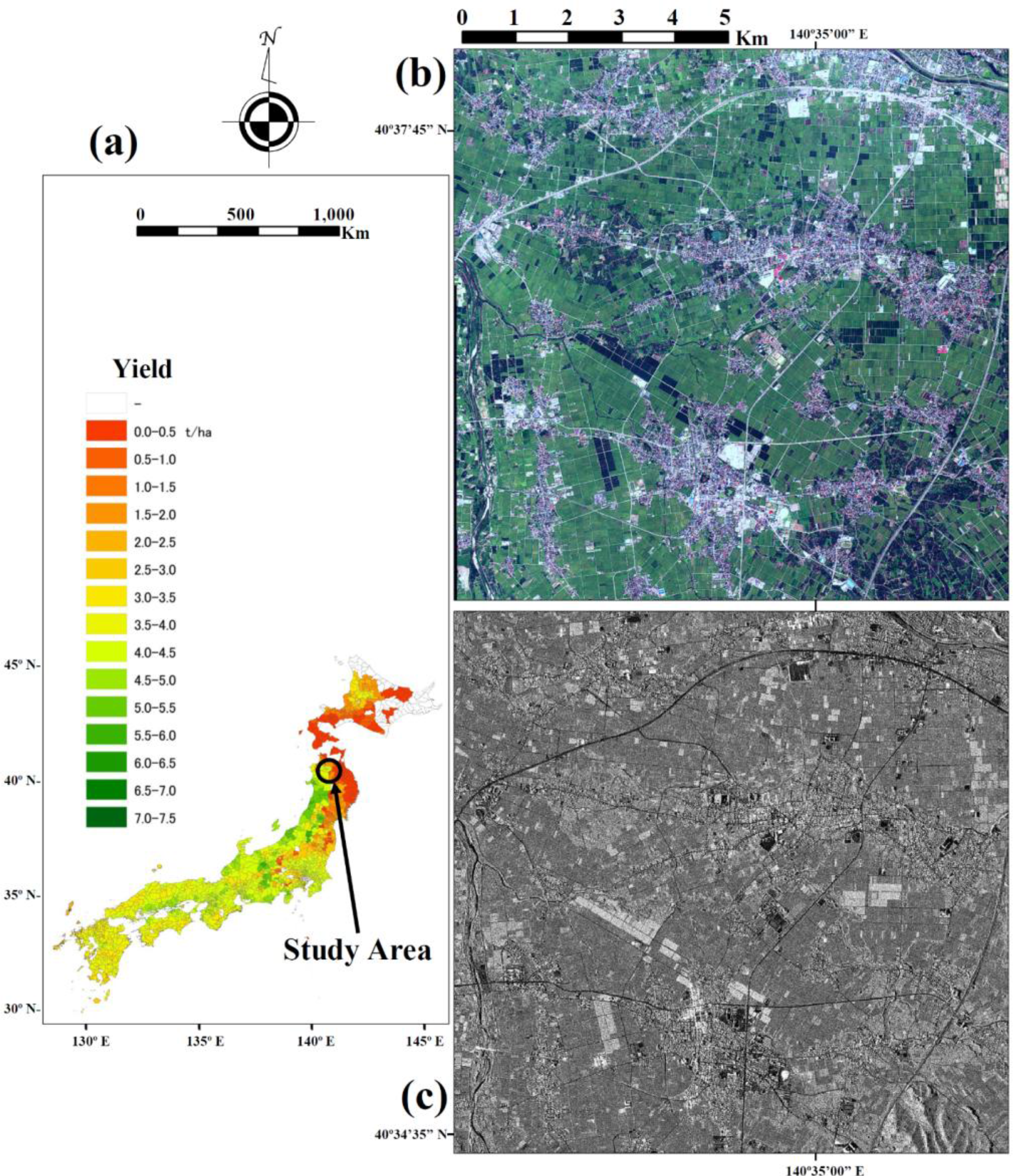
2.1. Study Site

A study site was selected in one of the major rice-growing regions in northeast Japan (Tsugaru Plain, Aomori Prefecture; center: 40°36′20.74″N, 140°33′36.02″E). Figure 1 depicts a part of the study area with an optical image (WorldView-2) and a SAR image (TSX) taken on the same day (2 September 2011). Rice yield in Japan is usually high and stable thanks to the advanced management technologies, but sometimes suffers from serious meteorological disasters as shown by a yield map in 1993 (Figure 1a) [38]. The area is flat and relatively uniform in its rice varieties grown and crop management practices. In general, rice is grown once a year during the summer season (May–September) in this region. The mean air temperature and total precipitation for the May–September period are 18.6 °C and 513 mm, respectively.
Normally, rice plants are transplanted in late May. Paddy fields are flooded several days before transplanting, and puddling/reveling is practiced one or two days before transplanting. The dates for the panicle initiation stage, heading stage, and maturing stage are mid-July, early-August, and mid-September, respectively. A single rice variety (Oryza sativa L. japonica, variety: Tsugaru Roman) is grown in the study area. In general, a bundle of 3–5 seedlings (hill) of about 15 cm long are machine planted at a spacing of around 30 cm × 15 cm under flooded conditions. Figure 2 shows the rice canopies at the early vegetative and mid-maturing stages. The maximum leaf area index (LAI) usually occurs around two weeks before heading stage. At the maturing stage, the number of panicles is equal to that of stems, so plenty of panicles are distributed at the top layer of a canopy (Figure 2b). Paddy fields are irrigated continuously until the mid-maturing stage, so the soil surface of paddy fields is under flooded conditions during most growing periods. Even in some periods without surface water, the soil surface is smooth and fully saturated with water. Although each rice field is highly homogeneous (coefficient of variation, CV for plant height <5%; Figure 2), between-field variability in growth and yield is significant because of differences in the soil condition and farming management practices. The majority of paddy fields in the study area have a size of 30 m × 100 m, but the orientation of fields (i.e., row direction) is not identical. The field size in the region is typical for Japan and most Asian countries, although it is much smaller than in the United States or European countries.

2.2. Acquisition and Processing of CSK and TSX SAR Images

Two X-band (9.65 GHz) satellite sensors, CSK and TSX, were used for the acquisition of high-resolution SAR images during four consecutive years. The main parameters of these images are summarized in Table 1. The overall information on crop conditions during each image-acquisition period is provided in the Table 1. In this study, we focused on the two specific growth stages, i.e., the transplanting period and the late maturing stage. The transplanting is one of the important events to be identified at a field scale for growth diagnosis and management from then onward. In addition, this event is useful to examine the response of X-band σ0 to a small change in paddy surfaces because transplanting causes a subtle but clear biophysical change on the surface. Accordingly, a TSX image was acquired during the transplanting season, i.e., on 26 May 2012. The late maturing stage was targeted because of two reasons; (1) it is an important growth stage for prediction of yield and/or grain quality; and (2) X-band was assumed to be effective to derive some unique information during the stage based on the previous study [23]. The second reason implies that the X-band σ0 is not suitable for estimating the whole canopy variables such as total biomass and leaf area during the most part of vegetative growth period because the volume scattering is easily saturated with a small volume of biomass, i.e., at an early growth stage [12]. In other words, from ecophysiological or agronomic points of view, acquisition of time-series images is not always useful to derive critical information for crop diagnosis. Hence, four X-band images were acquired during the late maturing stage, i.e., on 5 September 2009 (CSK), 8 September 2010 (CSK), 6 September 2011 (TSX), and 3 September 2012 (TSX), respectively.
Details of measurement configurations such as polarization and incidence angles were determined based mainly on the results of our previous study [23]. According to the results from combinations of all five frequency bands (Ka, Ku, X, C, L), four polarizations (VV, VH, HV, HH), and four incidence angles (25°, 35°, 45°, 55°), the X-band at a high incidence angle proved to have a significant relationship with canopy variables such as panicle weight. The spotlight mode was considered the most suitable mode for investigating the relationship of SAR data with canopy biophysical variables, considering the degradation of resolution due to noise-reduction processing as well as the small field size and the size of study area (100 km2; 10 × 10 km). Therefore, the spatial resolution (azimuth × ground range) for the selected mode was 1 m × 1 m for CSK, and 1.7 m × 1.48 m for TSX, respectively. The spatial resolution on the ground can be affected by the incidence angle to some extent, but the variability was small because of the small scene size. Since, in both X-band sensors, a single-polarization was selectable for the above spatial resolution and scene size, we selected the VV-polarization and shallow incidence angles, i.e., 54° (CSK) and 49.5° (TSX) for maturing period, and 44° (TSX) for transplanting period. Since the possible local time of satellite observation was limited to around 5:40 and 17:30 in both sensors, we selected the evening observations (17:30) to avoid the effects of morning dew except for the transplanting season. Potentially, the difference of pass, i.e., ascending or descending, may affect the backscattering in response to row directions of paddy fields. Nevertheless, judging from the uniform canopy surfaces during the maturing stages (e.g., in Figure 2b), we assumed the effect would be negligible at these growth stages, especially at shallow incidence angles.
All image data were converted to σ0 signatures based on the radiometric parameters provided for each dataset using Next ESA SAR Toolbox (NEST) 4B (European Space Agency, Paris, France). A 10 m resolution DEM dataset developed by the Geospatial Information Authority of Japan (GSI) was used for the basic geometric correction. To accurately identify the area of ground measurements, all images were georeferenced using high-resolution airborne images (1 m) obtained by the CASI hyperspectral sensor. A 3 × 3 enhanced Lee filter was applied to each image to reduce speckle noise because we found little difference between 3 × 3 and 5 × 5. Usually, the noise reduction sacrifices the spatial resolution, but the high-resolution capability of the sensors allowed the extraction of signatures for the area of interest (AOI) in each paddy field where the plant samples were taken. Actually, we found little difference between the average σ0 values for individual AOIs with and without noise reduction filters. The AOIs were selected carefully to ensure the homogeneity and to avoid the effects of field edge.

2.3. Ground-Based Data Acquisition

Since one of the focal points in this study is to investigate the comprehensive relationships of X-band σ0 with canopy biophysical variables, we obtained a range of ecophysiological or morphological canopy variables concurrently with the SAR observations during the four-year period. In addition, transplanting dates were identified in a large number of paddy fields by field-survey to investigate the response of σ0 to paddy surface conditions and water surfaces during the transplanting period.

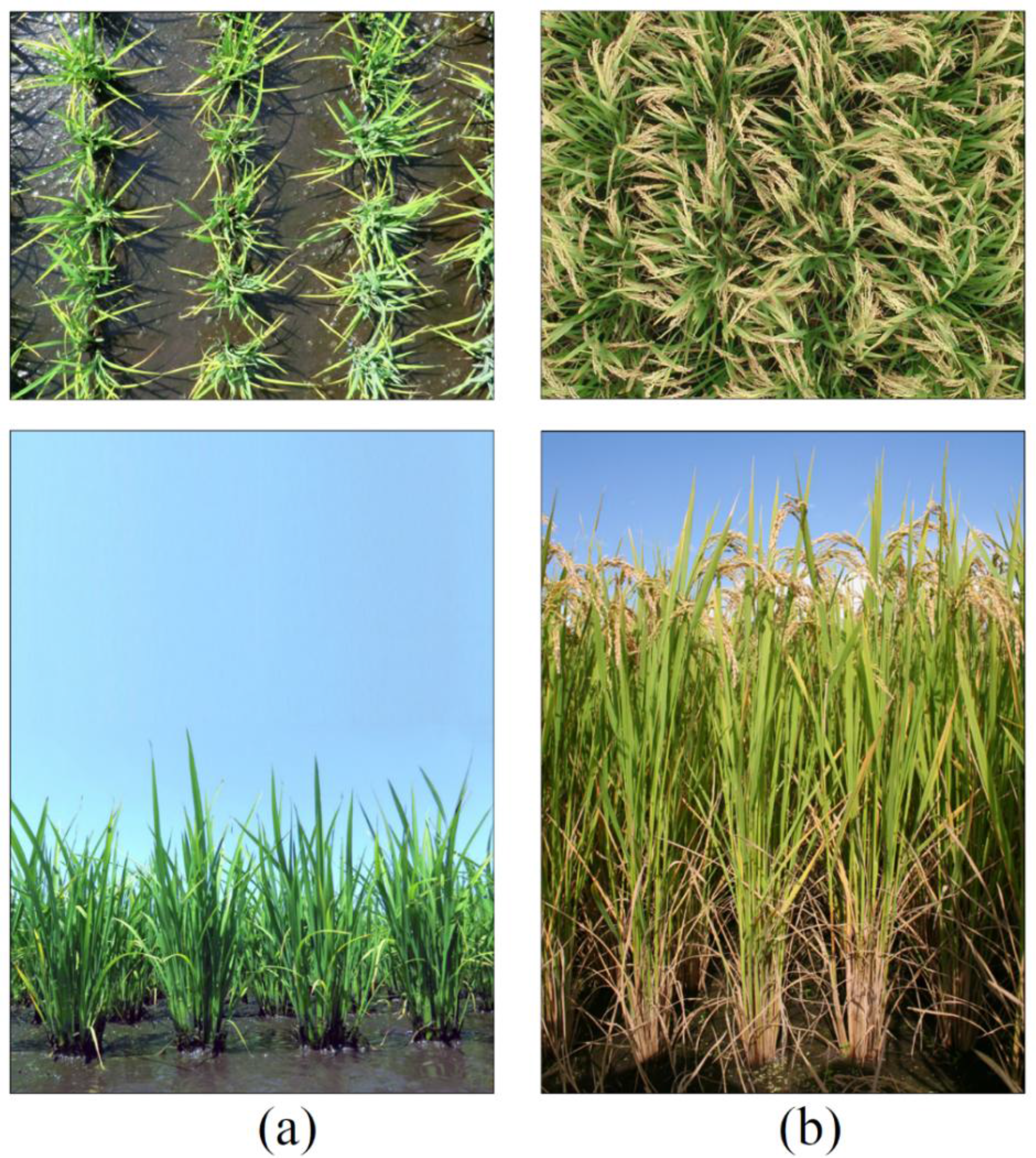
2.3.1. Biophysical Measurements of Rice Canopies

Ground-based measurements were made concurrently with the SAR observation at 36, 24, 38, and 33 paddy fields in 2009, 2010, 2011, and 2012, respectively. Hill density, plant height, and water depth were recorded for each field. Leaf chlorophyll content was estimated using a chlorophyll meter (SPAD502, Minolta). The fraction of photosynthetically active radiation (PAR) absorbed by the canopy (fAPAR) was determined based on the ascending and descending values of photosynthetic photon flux density (PPFD) measured at the top and bottom of a canopy using a line PPFD sensor (LI-191, Li-Cor).
Rice plants in individual fields were highly uniform, so five representative hills (a bundle of plants) were sampled from each paddy field to characterize the biophysical structure of the canopy. The wet and dry biomass of leaves, stems, panicles, and whole plants were determined by destructive measurements of the sampled plants. In addition, structural variables such as stem density, LAI, panicle size, leaf size (length, width, and thickness), number of leaves per stem, vertical position of panicles and leaves, and stem diameter were measured. These data were used for statistical analysis and as model inputs to a canopy backscattering model.

2.3.2. Determination of Transplanting Date in Individual Rice Paddies

Transplanting dates were identified in 640 individual paddy fields covered by the image (TSX on 26 May 2012) based on daily field-survey throughout the transplanting season. In addition, the actual paddy surface conditions of individual rice paddies before and after the transplanting event were recorded with photographs (e.g., pictures in Figures 2 and 3). The field survey enabled us to identify a variety of paddy-surface conditions within the SAR image, i.e., from plowed (dry) to transplanted conditions through flooding, puddling and transplanting. These data were given to the field-polygons as attributes on geographic information system (GIS), and used to examine the response of σ0 to water surfaces as well as to paddy surfaces with and without rice plants.

2.4. Analytical Approaches

2.4.1. Extraction of σ0 Values from SAR Images and their Statistical Analysis

In each SAR image, the σ0 values were extracted for the individual areas of interest in paddy fields (around plant-sampling point) as well as for nearby water surfaces (ponds and rivers), asphalt surfaces and urban areas. We assumed that the still-water surfaces, asphalt surfaces and urban areas would be most suitable as reference targets in image-to-image comparison because they would not be affected by vegetation, soil moisture, and wind conditions. Water and asphalt polygons were selected in uniform areas without disturbances. Urban polygons were selected in typical built areas without obvious temporal changes. The urban areas would include some asphalt surfaces, but we assumed them as another representative category of stable areas by taking much larger sizes.
In each image, more than 20 polygons were generated for each category based on the field-survey and optical satellite images. Consequently, the average size of polygons was 126,000 m2 for urban areas, whereas it was 5500 m2 for asphalt surfaces, 880 m2 for water surfaces, and 780 m2 for plant-sampling plots, respectively. These polygons were used to extract σ0 values from the four images obtained during the maturing stage. Additionally, a polygon dataset generated for all paddy fields in the study area (approximately 15,000 fields) was used to extract the field-average values of σ0 from the TSX image obtained during the transplanting season (26 May 2012).In order to avoid the edge effects as well as the possible effects of inaccuracy in polygon boundary, a 5 m buffer-area inside the polygon boundary was excluded to compute the representative field-average.
An image analyzing system (Imagine 2011, ERDAS) and a geographic information system (ArcGIS 10.0, ESRI) were used for processing of image data.
Characteristics of the σ0 values from CSK and TSX, and their relationship with biophysical variables were analyzed statistically using correlation and regression methods. The first focal point of this study, i.e., the difference and consistency of CSK and TSX, was investigated using the σ0 data extracted for water surfaces, paddy fields, asphalt surfaces and urban areas. In addition, the σ0 data for 640 individual fields with known transplanting date (see Section 2.3.2) were used to examine the basic response of X-band σ0 to rice paddies before and after the transplanting event. By this approach, a single SAR image can be used to derive the chrono-sequential response of X-band σ0 to the daily change of paddy conditions during the transplanting season, i.e., from coarse plowing to initial growth stage through flooding, puddling, leveling, and transplanting.
On the basis of these analyses, the second focal point of this study, i.e., the comprehensive relationships of X-band σ0 with the biophysical rice variables, was investigated using each dataset from CSK and TSX. Since we found a systematic bias between the σ0 values from CSK and TSX, we made a simple linear correction using an approach similar to Pettinato et al. [37] (see Section 3.3). Then, we further examined the response of X-band σ0 to biophysical variables using the combined dataset (CSK + TSX) to explore more general and robust relationships.

2.4.2. A Simple Canopy Backscattering Model in Support of Experimental Analysis

A physically-based canopy scattering model was used to simulate the backscattering coefficient of a rice canopy. In general, such simulation studies allow us to examine the signal response to the change of canopy biophysical variables and the effects of sensor configurations such as frequency, polarization and incidence angle. Accordingly, the use of physically-based model is very useful to investigate the theoretical soundness of the experimental results. Here, we examined the response of canopy σ0 under observed biophysical conditions using the model.
Details of the model structure are given in Wang et al. [27] and Karam et al. [39]. In brief, the model integrates the major scattering processes in a rice canopy with several assumptions; (1) the ground surface is a smooth surface with dielectric constant of water since paddy fields are flooded during the growing season; (2) a rice canopy consists of three layers (i.e., panicle-, leaf-, and stem-layers); (3) panicles and stems are expressed as short cylinders; (4) leaves are expressed as narrow and long ellipses; and (5) the leaf angle distribution is expressed by a specific probability distribution function with a few parameters. Accordingly, the total backscattering coefficient from a canopy (σtotal) is expressed as a linear combination of volume scattering from each component, its double bounce with ground, and ground surface scattering (in power unit):
σ total = σ leaf + σ leaf-ground + σ stem + σ stem-ground + σ panicle + σ panicle-ground + σ ground
where the σleaf, σstem, and σpanicle are volume scattering of leaves, stems, and panicles, respectively. The σleaf-ground, σstem-ground, and σpanicle-ground are double bounce between each component and ground. The σground is ground surface scattering [27].
The model has some inherent limitations due to the simplification of 3-D structure and biophysical characteristics of plant canopies. Predictive accuracies in forward simulations may not be high. Retrieval of canopy variables by model inversion may be still difficult. However, we assumed that the physically-based model would be useful to assess the relative response of σ0 components under a given configuration of SAR sensor. The necessary inputs and parameters were derived from the ground-based measurements (see Section 2.3) and default values adapted to X-band.

3. Results and Discussion

3.1. Difference and Consistency of σ0 Values from CSK and TSX

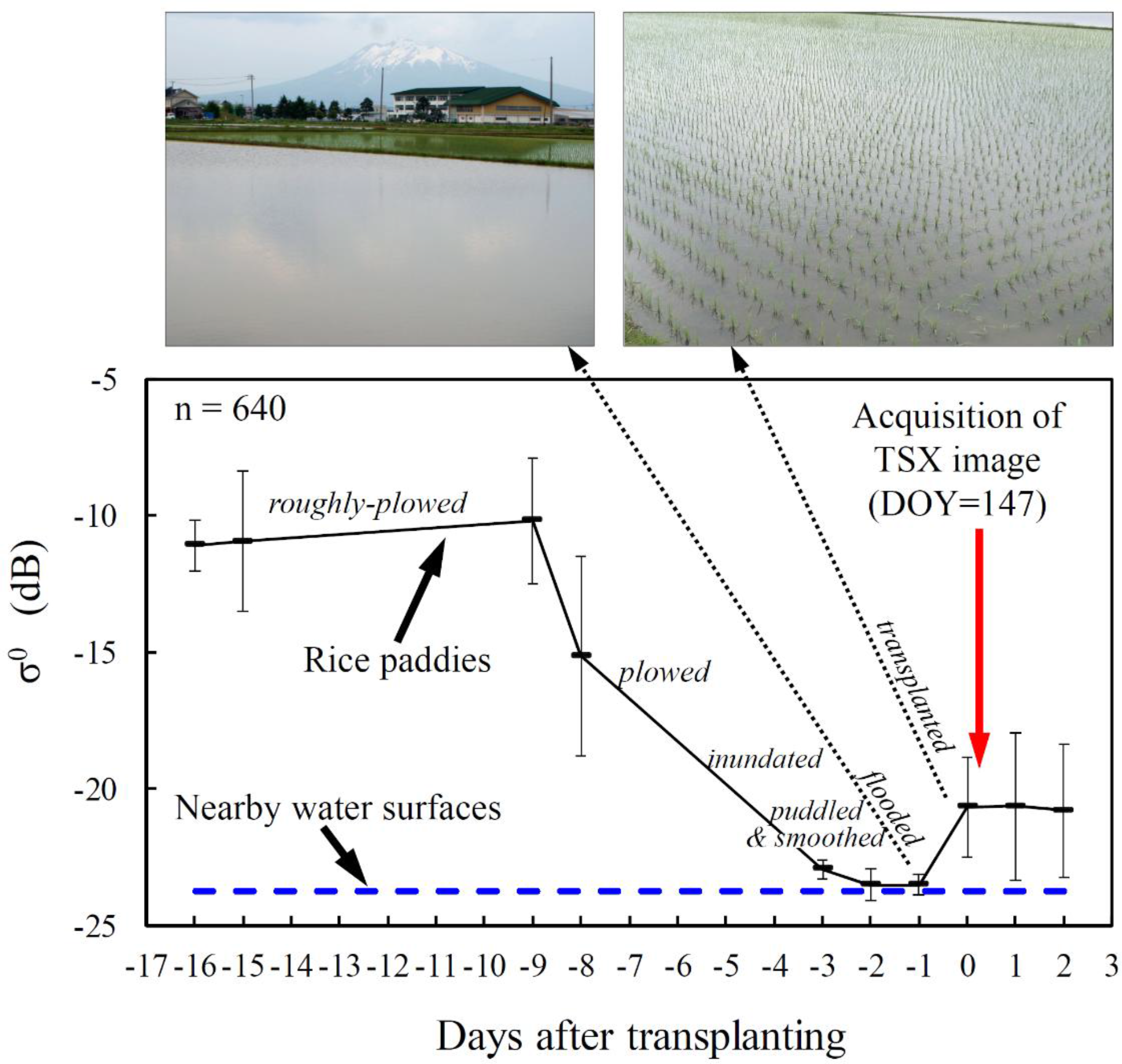
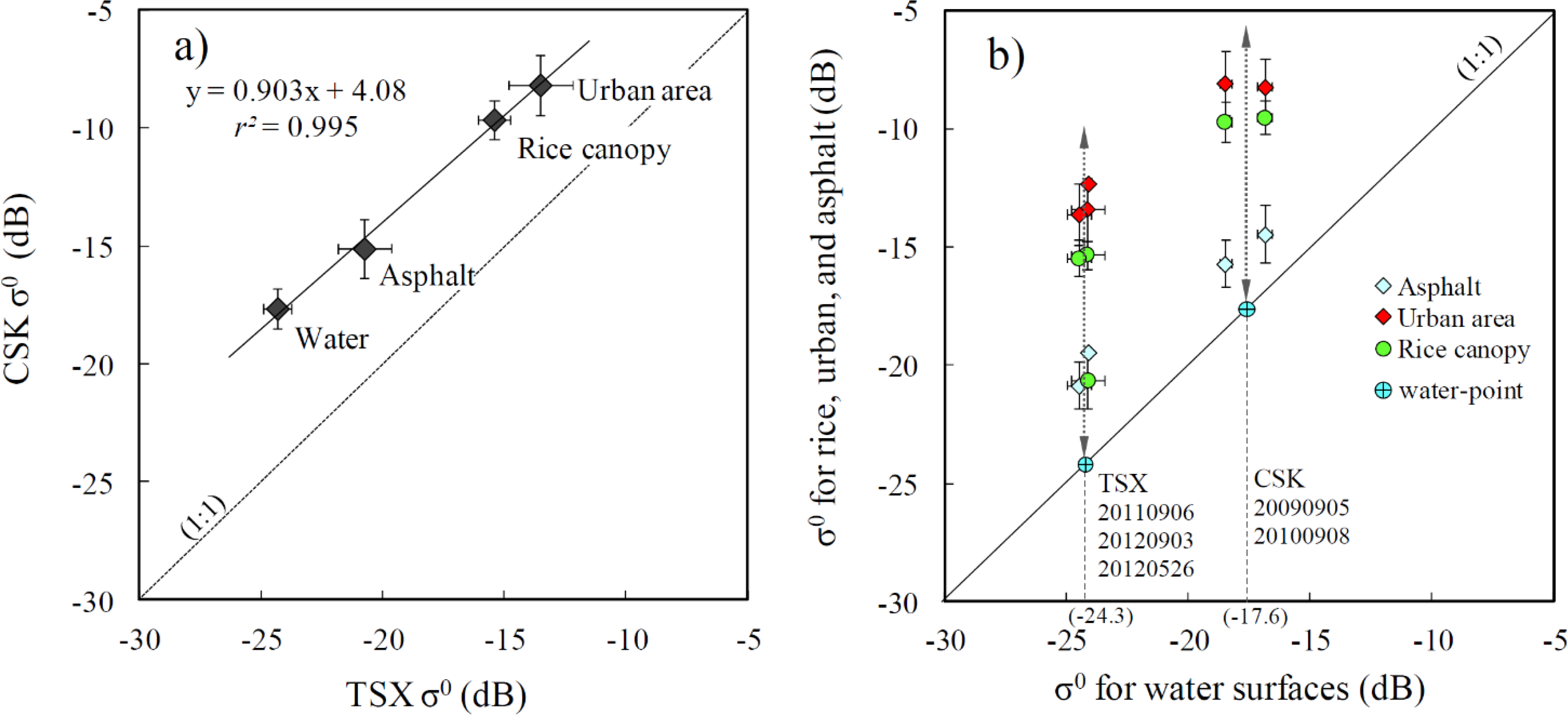
3.1.1. Response of σ0 to Transplanting and Water Surfaces

First, we investigated the chrono-sequential change of σ0 values of rice paddies extracted from the TSX image acquired during the transplanting season. The transplanting season is most suitable to examine the response of X-band σ0 to subtle amount of vegetation and to water surfaces. According to the scatterometer results by Inoue et al. [23], X-band σ0 shows a remarkable increase with transplanting, and then saturates at the early growth stage. Figure 3 shows the σ0 values of 640 rice paddies on the axis of days after transplanting (DAT). Since the TSX image was obtained in the morning of DOY 147 (26 May 2012), the DAT = +1 and DAT = −1 correspond one day after and before the transplanting, respectively. In other words, the line for rice paddies in the graph traces the chrono-sequential change of σ0 from plowed conditions (left) to transplanted conditions (right), through inundated, puddled/smoothed, and flooded conditions. The σ0 value changes significantly with transplanting by about 3 dB on average. The upper pictures show some examples of paddies before and after transplanting. This graph clearly indicates that the paddy surfaces just before transplanting have nearly the same σ0 values as the average σ0 for water surfaces (dotted line; −23.8 dB).
These results agree well with the experimental study using a ground-based scatterometer [23] showing that high frequency bands (Ka, Ku, X) can detect the subtle changes of a paddy surface due to the transplanting of thin rice seedlings (15 cm long) spaced at 30 cm × 15 cm. The subtle change is almost negligible in terms of biomass and is therefore hard to detect using optical sensors, but the X-band would be able to detect the small change with transplanting (Figure 3). The absolute change of σ0 caused by transplanting was relatively small compared to the scatterometer results (∼10 dB), but the difference may be attributable to differences in incidence angles as well as the sensitivity and noise level of the two systems. Spatial averaging may also affect the sensitivity in case of airborne or spaceborne SAR. The spatial averaging is effective in reducing the speckle noise, but would sacrifice the sensitivity. In general, the area size of spatial averaging should be balanced with the desired spatial resolution to obtain the sufficiently informative distribution of representative values of interest.
In applications of SAR images to assessment of planted area, usually a set of two SAR images obtained just after transplanting (first image) and a few months later (second image) is used to discriminate between rice and non-rice fields. Since the sensitivity of σ0 to initial growth differences depends on the frequency (Ka > Ku > X > C > L), the lower frequency bands (C, L) would need a longer time (i.e., a larger amount of growth) to discriminate the planted area. However, our results suggest that the high sensitivity of X-band SAR sensors to transplanting would make it possible to determine the date of transplanting instead of simply determining whether a field is planted if a few consecutive images are available during the transplanting season. Determination of planting date is strongly required by crop growth models for accurate assessment and prediction of growth and yield. Hence, the results obtained here would be applicable to large areas in Asia where transplanting is a common process in rice cultivation (e.g., 98.8% of rice area in Japan is by transplanting) according to the agricultural statistics [38]. However, note that, in rice production, there are several cultivation methods such as direct seeding.

3.1.2. Intercomparison of σ0 from CSK and TSX

Figure 4 compares the average σ0 values in four different types of surface (asphalt, urban area, rice canopy, and water) extracted from the CSK and TSX images during the maturing stage. This graph suggests that the σ0 values from each sensor are stable and consistent, respectively, even though all images were taken in different years. However, Figure 4a clearly shows that σ0 of CSK is higher than that of TSX. Judging from the near-parallel regression line to 1:1 line and the small error bars for all four categories, the bias between CSK and TSX would be a systematic difference. Figure 4b shows the relationship of σ0 values for rice, asphalt and urban surfaces against those for water surfaces. The average σ0 values of water surfaces from each sensor were consistent over the two years, i.e., −17.7 dB for CSK and −24.3 dB for TSX. This CSK-to-TSX difference (6.6 dB) may be specific to the configuration (spotlight mode, VV, 50°–54°) in our study, but all data in Figure 4 suggest the stability of the signatures from both sensors. The CSK-to-TSX difference here is much clearer than those reported by Pettinato et al. [37] for the other modes (Himage, Ping Pong, and Stripmap modes). They concluded that σ0 from Stripmap-TSX was higher than σ0 from Himage-CSK by 3.15 dB, and σ0 from Himage-CSK was higher than Ping Pong-CSK by 2.4 dB. These experimental results suggest that the CSK-to-TSX difference would vary significantly depending on acquisition modes and/or configurations. Some other preliminary studies on the discrepancy between the two sensors also support our insight, e.g., [36]. These differences may be attributable to some systematic differences in calibration procedures between the two sensors.
Figure 4b indicates that the distance of data points for asphalt, rice and urban areas from the 1:1 line was stable despite differences in years and sensors. Overall, the distance was approximately 3.0, 8.4, and 10.1 dB for asphalt, matured-rice, and urban areas, respectively. Note that the lowest point for rice (−21 dB) for TSX represents the average σ0 just after transplanting (Date: 26 May 2012, see Figure 3). Accordingly, we can assume that the position of σ0 for various surfaces would move along the dotted arrows (vertical lines for water surfaces) in each image. This is also supported clearly by the temporal change of σ0 derived from the different analysis (Figure 3). Note that the TSX σ0 values for water surfaces indicated in Figures 3 and 4 are very close to each other (−23.8∼−24.3 dB) despite the significant differences in season, year, and incidence angle. So, hereafter, we refer to the vertical line for water surfaces as “water-line”, and the intersection point between the water-line and 1:1 line is referred to as “water-point”.
Our results suggest that, even if the absolute σ0 values are not consistent between sensors and/or images, the difference of σ0 from the “water-point” would be used commonly for quantitative rice monitoring. Ideally, differences between sensors due to calibration problems should be solved systematically. However, this image-based approach is simple and robust, so it would be a useful approach in constellation-use of different SAR sensors towards timely and consistent crop monitoring. The “water-point” approach assumes that still-water surfaces are available within each image. This assumption may be applicable to most paddy rice-growing regions in monsoon Asia where a number of water bodies such as ponds, lakes, or rivers are found. Rippling waves due to strong wind can affect the σ0 to some extent, e.g., [11,23], but it would be possible to find still-water surfaces within each whole image as in our study. In general, vegetation and soil moisture conditions are critical confounding factors in selection of reference surfaces for image-to-image comparisons. Therefore, use of still-water surfaces as a reference for stable and minimum σ0 would be reasonable for this application. For the “water-point” method, the extraction of σ0 for still-water areas and identification of such areas in each image would be automated using the statistical frequency distribution of σ0 for the image and some indicators about the spatial extent of a specific value of σ0.

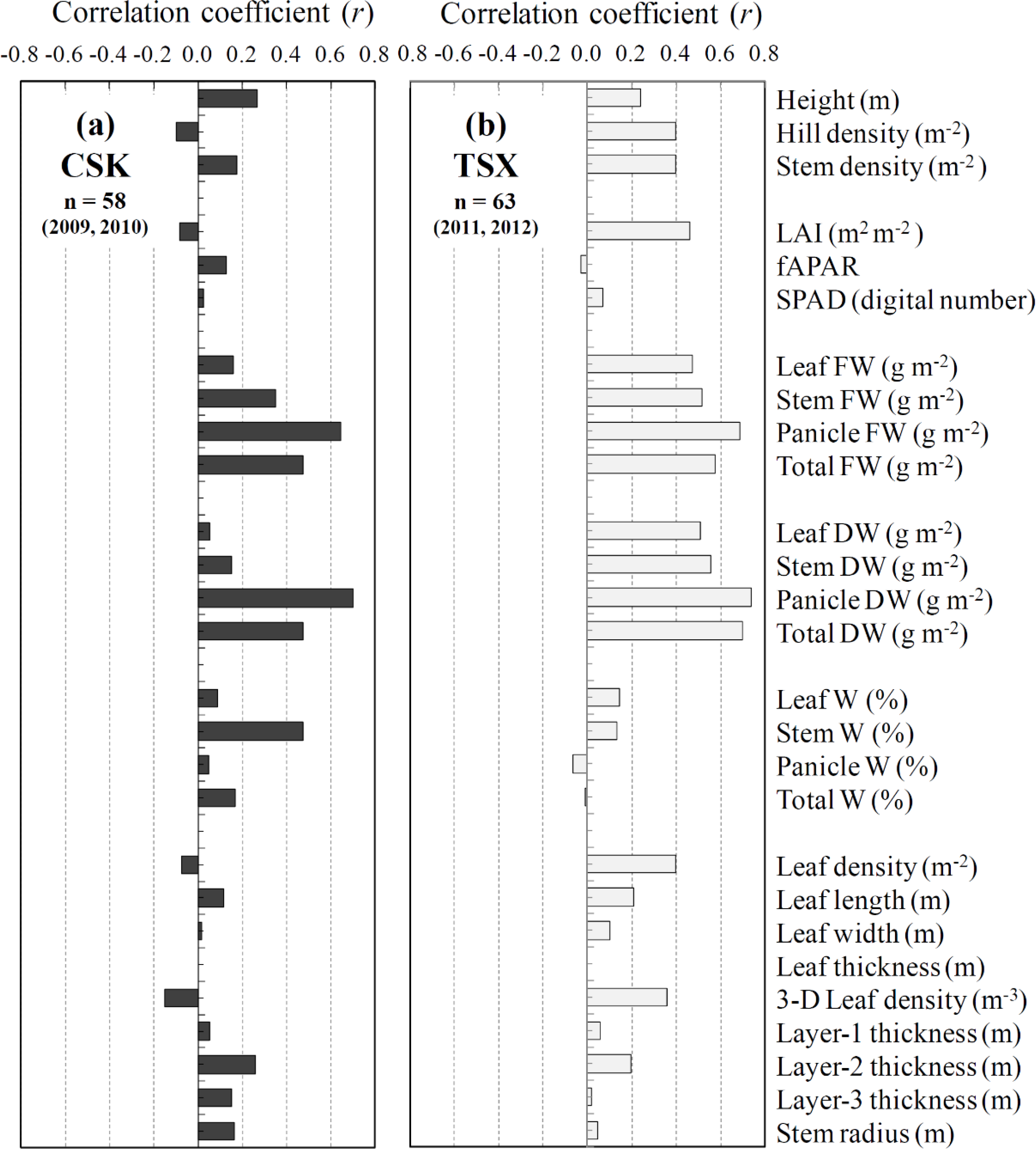
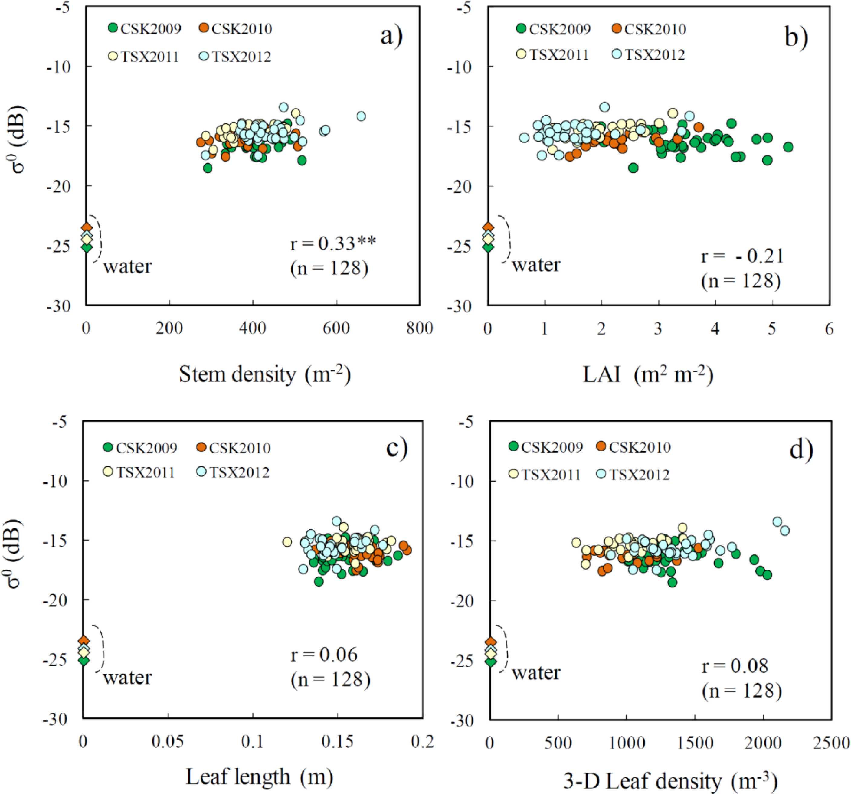
3.2. Relationships between the X-Band σ0 and Canopy Biophysical Variables

3.2.1. Analysis Using the Datasets for CSK and TSX

The results of a comprehensive statistical analysis on the relationship of the X-band σ0 with canopy biophysical variables are shown in Figure 5. The preliminary results for the CSK sensor (Figure 5a) from Inoue and Skaiya [12] are included for comparison of the two different sensors. Overall, the σ0 from TSX had a close positive relationship (at significance level of 0.01) with a larger number of canopy variables (13) than CSK σ0 (6). Among them, five variables (Stem FW, Panicle FW and DW, Total FW and DW) were common to TSX and CSK. The major target variable in this study, i.e., the panicle weight, was included in them as we presumed from the results by Inoue et al. [23]. Majority of the whole-canopy variables such as LAI, stem density, height, and fAPAR was not adequately correlated with σ0 values. The poor sensitivity of X-band σ0 to the whole-canopy variables is reasonable because it saturates at an early stage of rice growth. Ecophysiological and morphological variables such as chlorophyll content (SPAD), water content, and leaf length and width were poorly correlated with σ0. These results suggest the inherent limitation of X-band σ0 to detect the actual difference of biophysical variables because of its shallow penetration depth into a canopy. We believe that these negative results are also useful since the scientific knowledge on both ability and inability is critical for appropriate targeting in future research. Hopefully, other analytical techniques such as polarimetry, and multiangular measurements might provide useful information.
In Figure 5, we found that the most significant relationship common to CSK and TSX sensors was that between σ0 and the panicle biomass. The panicle dry weight (panicle DW) was most closely correlated with σ0, and the fresh weight (panicle FW) was the second most closely correlated. Considering the various confounding factors under field conditions such as row orientation, and soil surface and wind conditions, the correlation coefficient was considered to be high (significance level: 0.005). In general, scattering at the top layer of a canopy is dominant in the X-band, so that the X-band σ0 is strongly affected by the size and number of panicles, rachis branches, rice grains, and flag leaves within the surface layer of a canopy. This is clearer in VV than in HH owing to the difference in extinction process. The high sensitivity of X-band σ0 to panicle biomass may be explained by the fact that rachis branches with several grains have nearly the same size as the wavelength of the X-band (3 cm). This finding for satellite sensors is well supported by a detailed scatterometer study on the ground [23]. The authors demonstrated that the X-band as well as the Ka-band (1.9 cm) and Ku-band (0.9 cm) were also highly sensitive to the panicle biomass, which may be for the same reason. The water content and inclination angle of panicles may affect σ0, but the influence on the variability of σ0 may be minor because the panicles tend to be uniform at this growth stage.

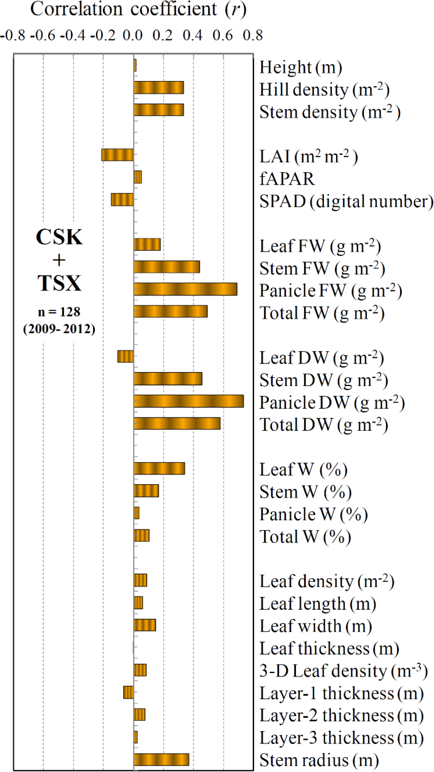
3.2.2. Analysis Using the Combined CSK and TSX Dataset

On the basis of the analysis in Figure 4, a systematic difference between CSK and TSX was corrected by subtracting the difference (6.6 dB) from the original σ0 values of CSK to create a combined dataset. Figure 6 shows the results of a comprehensive statistical analysis using the combined dataset.
Figure 7 shows scatter plots for the relationship of σ0 with four selected biophysical variables (stem density, LAI, leaf length, and 3-D leaf density). The σ0 values for the nearby water surfaces are shown on the y-axis for reference.
The results in Figures 6 and 7 provide interesting facts and useful insights. The overall tendency of the correlation coefficient in Figure 6 was similar to those for individual sensors (Figure 5). The most significant relationship was found for the panicle biomass. It is obvious that the differences in canopy height and fAPAR during the maturing stage were not detectable by σ0 because of the poor relationship between these variables. Figure 7 depicts a clear gap between the water surfaces and rice canopies even for the smallest values of stem density or LAI. These results were considered to be reasonable given that the high-frequency bands, especially at VV and shallow angle, are not able to penetrate into a rice canopy, especially during the maturing stage when large amounts of leaves, stems, and panicles are distributed near the canopy surface [23]. Accordingly, the X-band σ0 is most sensitive to the difference in the surface layer of a canopy during the maturing stage. In this stage, the most drastic change at the surface layer, i.e., grain filling, occurs without much change in the other parts.
In addition to the drastic change in panicle biomass, a significant change of 3-D geometry occurs during this period. Young panicles are near vertical at the heading stage, but bow down to the mixture of vertical and horizontal components at the full-maturity stage. However, it may be reasonable to assume that VV is more sensitive to the difference of panicle biomass compared to HH because the vertical component is dominant during the most part of maturing stage. The vertical and horizontal components are similar at the full-maturity stage, but still the difference of sensitivity between VV and HH would be minor, according to the scatterometer results by Inoue et al. (2002) [23].
The total biomass, stem density, or stem biomass had a certain positive relationship with σ0. However, their correlations would be indirect or superficial ones caused by the close ecophysiological relationship between such whole canopy variables and the panicle biomass. Interestingly, despite the no sensitivity of microwaves to the plant pigments (greenness), a negative significant correlation was found in green LAI and SPAD (Figure 6). This superficial correlation can also be explained by the negative ecophysiological relationship between the panicle growth and the leaf senescence. Both LAI and SPAD have relatively lower values in more matured canopies (larger panicle biomass).
The difference in water content cannot be detected by X-band σ0 because of the poor sensitivity (at most r = 0.35 for leaf W). Figure 6 also suggests that X-band σ0 is not sensitive to most of the other structural and morphological variables, such as leaf size and layer thickness although the sensitivity may be somewhat different for the other polarizations [26]. Above results suggest that the X-band SAR would have limited capability to assess variables related to the whole canopy only during the very early growth stages.

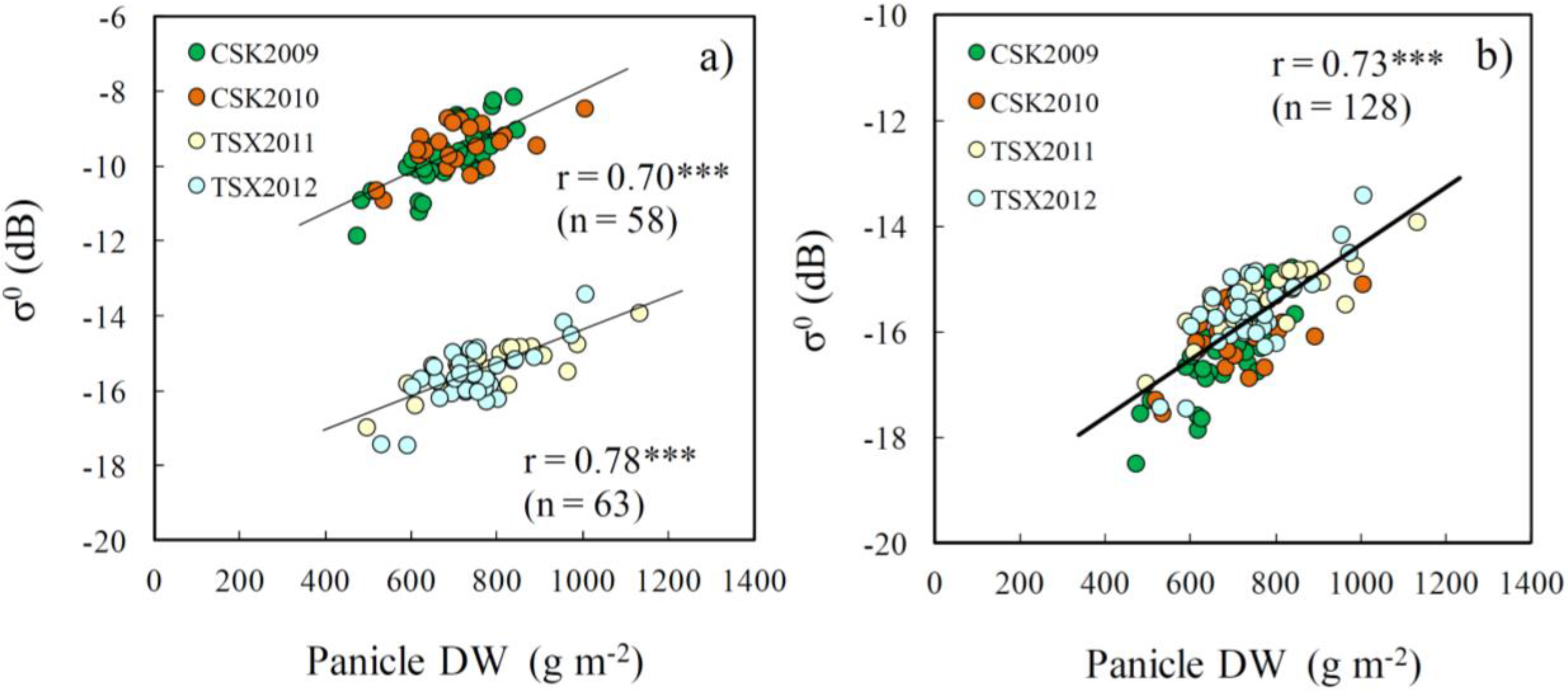
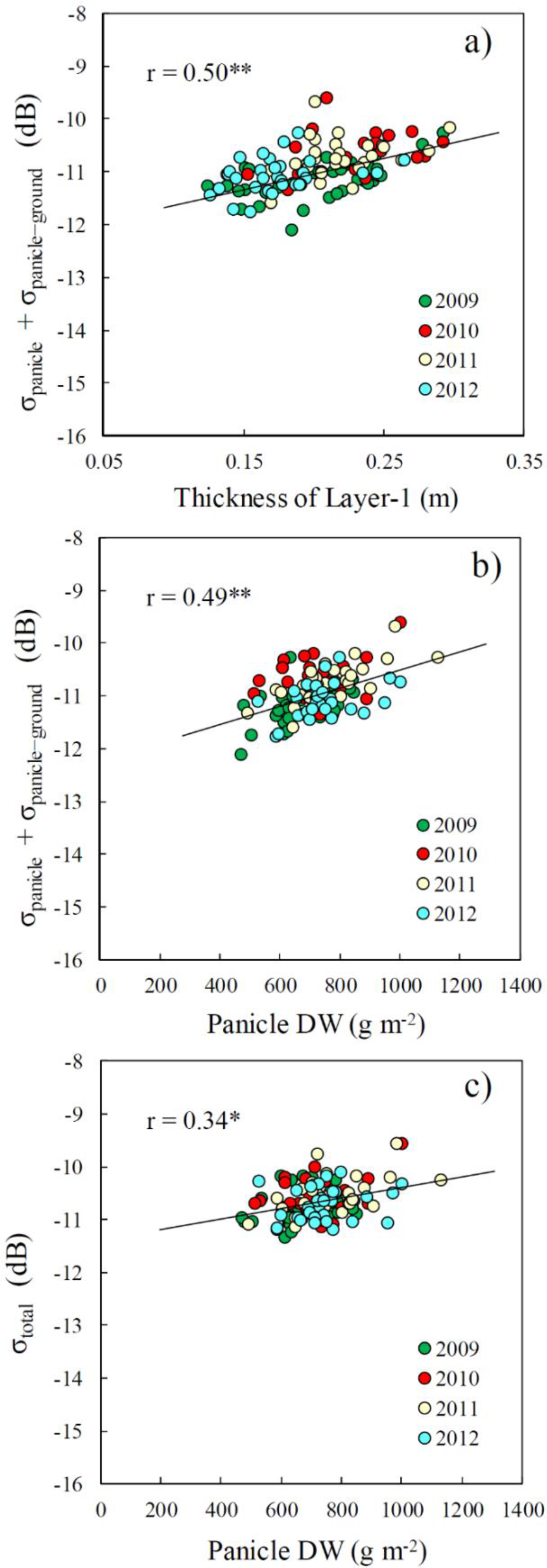
3.2.3. Examination of the Close Relationship of σ0 with Panicle Biomass

The close relationship between σ0 and the panicle dry biomass are examined based on the scatter plots for the individual CSK or TSX datasets and the combined dataset of CSK + TSX (Figure 8). This scatter plot for the two sensors over the four years strongly suggests a robust relationship between X-band σ0 and the panicle dry biomass despite the obvious difference in absolute σ0 values from the two sensors. The most important finding here is that the two regression lines for CSK and TSX (Figure 8a) are nearly parallel and accordingly the regression line for the CSK + TSX dataset (Figure 8b) keeps similar slope and correlation coefficient. The statistical probability was more than 99.5% significant.
These results strongly support the soundness of the image-based approach using the “water-point” proposed in previous Section 3.1.2, because the regression line in Figure 8b is equivalent to that for a combined CSK + TSX dataset of difference σ0 values between canopies and water surfaces in each image. Therefore, the approach based on the distance from the “water-point” along “water-line” (depicted in Figure 4) would be promising for quantitative monitoring of canopy biophysical variables using different sensors. In general, the panicle biomass (yield) had a close positive relationship with whole canopy variables such as total biomass. Accordingly, the total biomass, LAI, and fAPAR have been important targets for remote sensing studies because they are the key variables for plant productivity, e.g., [2,8,19,24]. However, from an ecophysiological point of view, yield is not always determined by the total biomass or LAI. For example, rice grain yield can be severely reduced despite the large canopy biomass or LAI because of abiotic and biotic stresses on reproductive organs. Sterility due to extreme temperatures or panicle blast sometimes causes significant yield reductions in monsoon Asia, e.g., [40]. In such cases, canopy biomass cannot be used as an effective indicator for estimating grain yield. However, even in such cases, the direct relationship found in this study may be a robust basis for estimating grain yield. Timely observation of rice canopies by X-band SAR sensors would provide an interesting opportunity to directly assess grain yield.
The relatively high correlation between the total biomass and σ0 found in this study (Figures 5 and 6) would be indirect or superficial, and attributable to the close relationship between the total biomass and panicle biomass [12], because the scattering process in the top canopy layer is dominant in the X-band, e.g., [22,23]. The sensitivity of σ0 to the panicle biomass was twice that of the sensitivity to the total biomass (5.5 and 2.5 dB·kg−1, respectively). Since a recent report clearly showed that C-band σ0 is promising for assessing LAI and fAPAR [13], a synergistic use of C- and X-bands would be more powerful for monitoring both the whole-canopy productivity and grain yield.

3.2.4. Analysis Using a Simple Canopy Scattering Model

The most interesting result, i.e., the relationship between X-band σ0 and panicle biomass, was investigated using a physically-based canopy scattering model (Equation (1)). Figure 9 shows the comparisons between simulated σ0 values (VV, 52°) and panicle-related variables. The panicle-related scattering component, σpanicle + σpanicle-ground, was moderately correlated with the depth of the panicle layer (Thickness of Layer-1; Figure 9a) and panicle biomass (Panicle DW; Figure 9b). The σtotal was also positively related with panicle biomass with somewhat lower coefficient. The difference in these correlation coefficients is reasonable because the σtotal is affected not only by panicle variables but also by many other factors such as leaves, whereas the σpanicle + σpanicle-ground is mainly determined by panicle variables. Overall, these results suggest that the experimental results obtained in Figure 8 would not contradict the backscattering processes integrated in the model. Although the absolute level of σ0 from the simulation did not agree well with the measurements, these simulation results may be useful to check the relative response of σ0 to the changes in canopy conditions.
In general, physically-based scattering models are based on many assumptions. Accordingly, the real canopy structures are greatly simplified. Moreover, it is difficult or often impossible to measure the accurate model-inputs in real canopies. Hence, we have to note that some discrepancies in absolute values and sensitivity between the experimental results in Figure 8 and the simulation results in Figure 9 suggest the limitations of the present model. The accurate measurement and modeling of 3-D distribution of rice panicles and their scattering processes would be one of the most interesting but challenging tasks in the future.

3.3. Overall Capability of X-Band σ0 and its Improvement for the Assessment of Biophysical Variables

Our experimental results based on datasets from two sensors over four years suggest a clear and consistent relationship between X-band σ0 and canopy biophysical variables. Because of the limited capability of the current sensors, the present analysis was based on the dataset at VV polarization and an incidence angle of around 50°. However, these results provide clearer insights regarding the capability of the other configurations, with the support of the comprehensive results previously obtained under a wide range of configurations [23].
The availability of multi-polarization measurement is still limited in most current satellite/modes. For this reason, the present study focused on a specific polarization (VV) considering the necessary spatial resolution and scene-size (coverage). However, full-polarimetric images will be available in high-resolution mode in the near future. More sensitive components of the signatures may then be explored for a more accurate assessment of the biophysical variables. Use of multi-polarization has proven effective for improving the accuracy of classification [13,18,19].
In this analysis, field or canopy conditions such as row orientation and ground surface conditions were not taken into consideration. Therefore, the accuracy of the assessment of biophysical variables from SAR signatures could be further improved by reducing the effects of confounding factors such as variability in incidence angle, row direction, and soil roughness.
Backscattering signals from vegetated surfaces are affected by many factors, including plant biomass, structure (e.g., leaf size, stem density, LAI), soil moisture, and roughness, as well as their interactions with sensor configurations, such as frequency, polarization, and incidence angle. Therefore, process-based models that take account of such factors are also useful for understanding and/or predicting the microwave backscattering processes in plant canopies, e.g., [22,27,39,41]. As mentioned in the previous Section (3.2.3), rice canopy structures are not incorporated sufficiently in physically-based models to examine the detailed interactions between biophysical variables and σ0. Future improvement of physically-based models would contribute to better interpretation and assessment of canopy biophysical variables.
The synergistic use of SAR and optical sensors is also effective in improving accuracy, e.g., [42,43]. For example, supplemental information for each field, such as shape, orientation, and fractional vegetation cover, can be obtained based on the segmentation of high-resolution multispectral images, e.g., [44,45]. In addition, the synergistic use of SAR sensors with different frequency such as L-, C- and X-band would be promising since they are sensitive to different canopy variables [13,20,23,26].
Although rice-cropping technologies in Japan are well modernized, the productivity of high-quality rice is still not stable, especially under recent climate change. The spatial and temporal variability is large (i.e., approximately 0–150% of the national average; e.g., Figure 1a), mainly due to adverse weather conditions. This variability is much larger in many other rice-growing countries in Asia. Hence, especially under monsoon conditions in Asia, microwave remote sensing has great potential for monitoring and predicting rice growth and yield for precision management and food security.

4. Conclusions

Our analytical results based on datasets from two satellite X-band SAR sensors (Cosmo-SkyMed and TerraSAR-X) over four years elucidate a clear and consistent relationships between the two sensors, as well as the potential of X-band σ0 sensors for monitoring rice biophysical variables.
The chrono-sequential change of σ0 in a rice paddy during the transplanting season (i.e., from plowed dry conditions to transplanted conditions through flooded and puddled/smoothed surface conditions) was revealed using a single SAR image. Results clearly indicated that paddy surfaces a few days before transplanting would have nearly the same σ0 values as water surfaces, and then the σ0 would change significantly (about 3 dB) with transplanting.
For both the CSK and TSX sensors, the backscattering coefficients σ0 in rice paddies, water surfaces, asphalt surfaces, and urban areas were stable and consistent for two consecutive years. However, a clear systematic shift (6.6 dB) was found between the two sensors. This difference would be attributable to calibration issues, and the difference would vary depending on acquisition modes. Most importantly, we found that the differences in σ0 between target surfaces and water surfaces in each image are comparable in all images from both sensors despite the obvious differences in absolute σ0 values. On average, the difference σ0 was 3.0 dB for asphalt, 8.4 dB for rice paddies, and 10.1 dB for urban areas, respectively. Accordingly, an image-based approach using the “water-point” has been proposed. This approach would be used commonly for quantitative rice monitoring, even if the absolute σ0 values are not consistent between sensors and/or images.
The X-band σ0 from both sensors were correlated with stem fresh weight, panicle biomass, and total biomass at high statistical significance. Among the various biophysical and morphological variables, the panicle biomass was found to be best correlated with X-band σ0 at VV polarization. This relationship was supported by simulations using a physically-based canopy scattering model. These results based on two different sensors clearly support the results of preliminary study by Inoue et al. [12] that X-band SAR would have potential for direct assessments of rice grain yields at regional scales from space. A close correlation was also found between the total biomass and σ0, but this may be an indirect relationship because of the close relationship between total biomass and panicle biomass. X-band σ0 did not appear to be very sensitive to most of the other structural and morphological variables, such as leaf size and layer thickness, during the maturing stage of paddy rice. These results suggest that the X-band SAR would have limited capability to assess the whole-canopy variables only during the very early growth stages.
Because of the limited capability of current sensors, the present analysis was based on a dataset at VV polarization and an incidence angle of around 50°. However, our experimental results based on detailed ground-based measurements would provide useful insights on the potential and limitations of satellite SAR sensors in general for agricultural and ecosystem applications. The constellation-use of multiple SAR sensors would greatly contribute to timely acquisition of crop information for precision farming and for decision making for food security.

Acknowledgments

This work was supported financially by the JSPS and MEXT, Japan. The authors are grateful to the efficient help by the technical staff with the National Institute for Agro-Environmental Sciences. We would like to thank Juan M. Lopez-Sanchez (University of Alicante, Spain) and Thuy Le Toan (CESBIO, France) for their helpful comments.

Author Contributions

Yoshio Inoue designed and conducted the analysis and wrote the manuscript. Yoshio Inoue and Eiji Sakaiya collected all the dataset with assistants of the technical staff. Cuizhen Wang assisted the simulation analysis using a backscattering model.

Conflicts of Interest

The authors declare no conflict of interest.

References

  1. Moran, M.S.; Inoue, Y.; Barnes, E.M. Opportunities and limitations for image-based remote sensing in precision crop management. Remote Sens. Environ 1997, 61, 319–346. [Google Scholar]
  2. Inoue, Y. Synergy of remote sensing and modeling for estimating ecophysiological processes in plant production. Plant Prod. Sci 2003, 6, 3–16. [Google Scholar]
  3. Doraiswamy, P.C.; Hatfield, J.L.; Jackson, T.J.; Akhmedov, B.; Prueger, J.; Stern, A. Crop condition and yield simulation using Landsat and MODIS. Remote Sens. Environ 2004, 92, 548–559. [Google Scholar]
  4. Becker-Reshef, I.; Justice, C.; Sullivan, M.; Vermote, E.; Tucker, C.; Anyamba, A.; Small, J.; Pak, E.; Masuoka, E.; Schmaltz, J.; et al. Monitoring global croplands with coarse resolution earth observations: The Global Agriculture Monitoring (GLAM) Project. Remote Sens 2010, 2, 1589–1609. [Google Scholar]
  5. Ishijima, K.; Sugawara, S.; Kawamura, K.; Hashida, G.; Morimoto, S.; Murayama, S.; Aoki, S.; Nakazawa, T. Temporal variations of the atmospheric nitrous oxide concentration and its δ15N and δ18O for the latter half of the 20th century reconstructed from firn air analyses. J. Geophys. Res 2007, 112, D03305. [Google Scholar]
  6. Nishio, M. Agriculture and Environmental Pollution—Technology and Policy for Soil Environment; Rural culture Association: Tokyo, Japan, 2005; p. 439. [Google Scholar]
  7. Inoue, Y.; Dabrowska-Zierinska, K.; Qi, J. Synoptic assessment of environmental impact of agricultural management: A case study on nitrogen fertilizer impact on groundwater quality, using a fine-scale geoinformation system. Int. J. Environ. Stud 2012, 69, 443–460. [Google Scholar]
  8. Le Toan, T.; Ribbes, F.; Wang, L.F.; Nicolas, F.; Ding, K.H.; Kong, J.A.; Fujita, M.; Kurosu, T. Rice crop mapping and monitoring using ERS-1 data based on experiment and modeling results. IEEE Trans. Geosci. Remote Sens 1997, 35, 41–56. [Google Scholar]
  9. Brisco, B.; Brown, R.J. Agricultural Applications with Radar. In Manual of Remote Sensing Principles and Applications Imaging Radar, 3rd ed; Henderson, F., Lewis, A., Eds.; Wiley: New York, NY, USA, 1998; pp. 381–406. [Google Scholar]
  10. Jackson, T.J. Remote Sensing Soil Moisture. In Encyclopedia of Soils in the Environment; Hillel, D., Ed.; Elsevier Ltd.: Oxford, UK, 2005; pp. 392–398. [Google Scholar]
  11. Lopez-Sanchez, J.M.; Ballester-Berman, J.D. Potentials of polarimetric SAR interferometry for agriculture monitoring. Radio Sci 2009, 44. [Google Scholar] [CrossRef]
  12. Inoue, Y.; Sakaiya, E. Relationship between X-band backscattering coefficients from high-resolution satellite SAR and biophysical variables in paddy rice. Remote Sens. Lett 2013, 4, 288–295. [Google Scholar]
  13. Inoue, Y.; Sakaiya, E.; Wang, C. Capability of C-band backscattering coefficients from high-resolution satellite SAR sensors to assess biophysical variables in paddy rice. Remote Sens. Environ 2014, 140, 257–266. [Google Scholar]
  14. Baldini, L.; Roberto, N.; Gorgucci, E.; Fritz, J.; Chandrasekar, V. Analysis of dual polarization images of precipitating clouds collected by the COSMO SkyMed constellation. Atmos. Res 2014, 144, 21–37. [Google Scholar]
  15. Kurosu, T.; Fujita, M.; Chiba, K. The identification of rice fields using multi-temporal ERS-1 C band SAR data. Int. J. Remote Sens 1997, 18, 2953–2965. [Google Scholar]
  16. Ribbes, F.; Le Toan, T. Rice field mapping and monitoring with RADARSAT data. Int. J. Remote Sens 1993, 20, 745–765. [Google Scholar]
  17. Choudhury, I.; Chakraborty, M.; Santra, S.C.; Parihar, J.S. Methodology to classify rice cultural types based on water regimes using multi-temporal RADARSAT-1 data. Int. J. Remote Sens 2012, 33, 4135–4160. [Google Scholar]
  18. Bouvet, A.; Le Toan, T.; Lam-Dao, N. Monitoring of the rice cropping system in the Mekong Delta using ENVISAT/ASAR dual polarization data. IEEE Trans. Geosci. Remote Sens 2009, 47, 517–526. [Google Scholar]
  19. Lopez-Sanchez, J.M.; Ballester-Berman, J.D.; Hajnsek, I. First results of rice monitoring practices in Spain by means of time series of TerraSAR-X dual-pol images. IEEE J. Sel. Top. Appl. Earth Obs. Remote Sens 2011, 4, 412–422. [Google Scholar]
  20. Lopez-Sanchez, J.M.; Vicente-Guijalba, F.; Ballester-Berman, J.D.; Cloude, S.R. Polarimetric response of rice fields at C-band: Analysis and phenology retrieval. IEEE Trans. Geosci. Remote Sens 2013, 52, 2977–2993. [Google Scholar]
  21. Bouman, B.A.M. Crop parameter estimation from ground-based X-band (3-cm wave) radar backscattering data. Remote Sens. Environ 1991, 37, 193–205. [Google Scholar]
  22. Prévot, L.; Champion, I.; Guyot, G. Estimating surface soil moisture and leaf area index of a wheat canopy using a dual-frequency (C and X bands) scatterometer. Remote Sens. Environ 1993, 46, 331–339. [Google Scholar]
  23. Inoue, Y.; Kurosu, T.; Maeno, H.; Uratsuka, S.; Kozu, T.; Dabrowska-Zielinska, K.; Qi, J. Season-long daily measurements of multifrequency (Ka, Ku, X, C, and L) and full-polarization backscatter signatures over paddy rice field and their relationship with biological variables. Remote Sens. Environ 2002, 81, 194–204. [Google Scholar]
  24. Shao, Y.; Fan, X.; Liu, H.; Xiao, J.; Ross, S.; Brisco, B.; Brown, R.; Staples, G. Rice monitoring and production estimation using multitemporal RADARSAT. Remote Sens. Environ 2001, 76, 310–325. [Google Scholar]
  25. Chakraborty, M.; Manjunath, K.R.; Panigrahy, S.; Kundu, N.; Parihar, J.S. Rice crop parameter retrieval using multi-temporal, multi-incidence angle Radarsat SAR data. ISPRS J. Photogramm. Remote Sens 2005, 59, 310–322. [Google Scholar]
  26. Lopez-Sanchez, J.M.; Cloude, S.R.; Ballester-Berman, J.D. Rice phenology monitoring by means of SAR polarimetry at X-band. IEEE Trans. Geosci. Remote Sens 2012, 50, 2695–2709. [Google Scholar]
  27. Wang, C.; Wu, J.; Zhang, Y.; Pan, G.; Qi, J.; Salas, W.A. Characterizing L-band scattering of paddy rice in southeast China with radiative transfer model and multitemporal ALOS/PALSAR imagery. IEEE Trans. Geosci. Remote Sens 2009, 47, 988–998. [Google Scholar]
  28. Baghdadi, N.; Zribi, M.; Loumagne, C.; Ansart, P.; Anguela, T.P. Analysis of TerraSAR-X data and their sensitivity to soil surface parameters over bare agricultural fields. Remote Sens. Environ 2008, 112, 4370–4379. [Google Scholar]
  29. Baghdadi, N.; Boyer, N.; Todoroff, P.; El Hajj, M.; Bégué, A. Potential of SAR sensors TerraSAR-X, ASAR/ENVISAT and PALSAR/ALOS for monitoring sugarcane crops on Reunion Island. Remote Sens. Environ 2009, 113, 1724–1738. [Google Scholar]
  30. Anguela, T.P.; Zribi, M.; Baghdadi, N.; Loumagne, C. Analysis of local variation of soil surface parameters with TerraSAR-X radar data over bare agricultural fields. IEEE Trans. Geosci. Remote Sens 2010, 48, 874–881. [Google Scholar]
  31. Canisius, F.; Fernandes, R. ALOS PALSAR L-band polarimetric SAR data and in situ measurements for leaf area index assessment. Remote Sens. Lett 2012, 3, 221–229. [Google Scholar]
  32. Fieuzal, R.; Baup, F.; Marais-Sicre, C. Sensitivity of TERRASAR-X, RADARSAT-2 and ALOS Satellite Radar Data to Crop Variables. Proceeding of the IEEE International Geoscience and Remote Sensing Symposium (IGARSS) 2012, Munich, Gremany, 18 July 2012; pp. 3740–3743.
  33. Gebhardt, S.; Huth, J.; Nguyen, L.D.; Roth, A.; Kuenzer, C. A comparison of TerraSAR-X Quadpol backscattering with RapidEye multispectral vegetation indices over rice fields in the Mekong Delta, Vietnam. Int. J. Remote Sens 2012, 33, 7644–7661. [Google Scholar]
  34. Santi, E.; Fontanelli, G.; Montomoli, F.; Brogioni, M.; Macelloni, G.; Paloscia, S.; Pettinato, S.; Pampaloni, P. The Retrieval and Monitoring of Vegetation Parameters from COSMO-SkyMed Images. Proceedings of the IEEE International Geoscience and Remote Sensing Symposium (IGARSS) 2012, Munich, Germany, 18 July 2012; pp. 7031–7034.
  35. Satalino, G.; Panciera, R.; Balenzano, A.; Mattia, F.; Walker, J. COSMO-SkyMed Multi-Temporal Data for Land Cover Classification and Soil Moisture Retrieval Over an Agricultural Site in Southern Australia. Proceedings of the 2002 IEEE International Geoscience and Remote Sensing Symposium (IGARSS), Munich, Germany, 18 July 2012; pp. 5701–5704.
  36. Paloscia, S.; Pampaloni, P.; Santi, E.; Pettinato, S.; Brogioni, M.; Palchetti, E.; Crepaz, A. Comparison of Cosmo-SkyMed and TerraSAR-X Data for the Retrieval of Land Hydropogical Parameters. Proceeding of the IEEE International Geoscience and Remote Sensing Symposium (IGARSS) 2012, Munich, Germany, 18 July 2012; pp. 5510–5513.
  37. Pettinato, S.; Santi, E.; Paloscia, S.; Pampaloni, P.; Fontanelli, G. The intercomparison of X-band SAR images from COSMO-SkyMed and TerraSAR-X satellites: Case studies. Remote Sens 2013, 5, 2928–2942. [Google Scholar]
  38. Ministry of Agriculture, Forestry and Fisheries of Japan (MAFF-J), Statistical Report on Agriculture and Forestry 2012; MAFF-J: Tokyo, Japan, 2012.
  39. Karam, M.A.; Amar, F.; Fung, A.K.; Mougin, E.; Lopes, A.; Le Vine, D.M.; Beaudoin, A. A microwave polarimetric scattering model for forest canopies based on vector radiative transfer theory. Remote Sens. Environ 1995, 53, 16–30. [Google Scholar]
  40. Nishiyama, I. Damage due to Extreme Temperatures. In Science of the Rice Plant; Matsuo, T., Kumazawa, K., Ishii, R., Ishihara, H., Hirata, H., Eds.; Food and Agriculture Policy Research Center: Tokyo, Japan, 1995; pp. 769–812. [Google Scholar]
  41. Ulaby, F.T.; Allen, C.T.; Eger, G.; Kanemasu, E.T. Relating the microwave backscattering coefficient to leaf area index. Remote Sens. Environ 1984, 14, 113–133. [Google Scholar]
  42. Moran, M.S.; Vidal, A.; Troufleau, D.; Qi, J.; Clarke, T.R.; Pinter, P.J., Jr.; Mitchell, T.A.; Inoue, Y.; Neale, C.M.U. Combining multifrequency microwave and optical data for crop management. Remote Sens. Environ 1997, 61, 96–109. [Google Scholar]
  43. McNairn, H.; Champagne, C.; Shang, J.; Holmstrom, D.; Reichert, G. Integration of optical and Synthetic Aperture Radar (SAR) imagery for delivering operational annual crop inventories. ISPRS J. Photogramm. Remote Sens 2009, 64, 434–449. [Google Scholar]
  44. Inoue, Y.; Kiyono, Y.; Asai, H.; Ochiai, Y.; Qi, J.; Olioso, A.; Shiraiwa, T.; Horie, T.; Saito, K.; Dounagsavanh, L. Assessing land use and carbon stock in slash-and-burn ecosystems in tropical mountain of Laos based on time-series satellite images. Int. J. Appl. Earth Obs. Geoinf 2010, 12, 287–297. [Google Scholar]
  45. Liu, D.; Xia, F. Assessing object-based classification: Advantages and limitations. Remote Sens. Lett 2010, 1, 187–194. [Google Scholar]
Figure 1. Study area. (a) A yield map of rice over Japan in a year (1993) of serious cold damage; (b) A natural color image taken by WorldView-2 on 28 August 2011; (c) A σ0 image taken by TSX on 6 September 2011.
Remotesensing 06 05995f1
Figure 2. Examples of rice canopies in the study area; nadir and side view of typical rice canopies at vegetative stage (a) and maturing stage (b). The right hand stage was targeted mainly in this study.
Remotesensing 06 05995f2
Figure 3. The σ0 values for various conditions of rice paddies plotted on the axis of days after transplanting (DAT). Date of transplanting was identified for 640 rice paddy fields within the image taken by TSX on 26 May 2012 (DOY 147). For example, fields for DAT +1 and −1 were under the conditions a day before and after transplanting, respectively. Upper pictures show the typical situation for the fields observed on DOY147.
Remotesensing 06 05995f3
Figure 4. Comparison of σ0 values in rice canopies, asphalt surfaces, urban areas, and water surfaces obtained by CSK and TSX sensors. (a) Comparison of average σ0 of the four categories in CSK and TSX images during the maturing stage; (b) Comparison of σ0 for rice, asphalt and urban areas against σ0 for water surfaces. Dates of SAR observations are indicated in yyyymmdd along the “water-line” for CSK and TSX, respectively. The water-point is the intersection point between water-line and 1:1 line.
Remotesensing 06 05995f4
Figure 5. Correlation of σ0 from CSK (a) and TSX (b) sensors with biophysical and morphological variables in rice canopies at maturing stage. SPAD: chlorophyll index by SPAD502; FW: fresh biomass; DW: dry biomass; W: water content; Layer-1, 2, 3: thickness of layers for panicles (1), leaves (2), and stems (3), respectively. The correlation coefficient (r) at significance level of 0.01 and 0.05 is 0.33 and 0.25, respectively.
Remotesensing 06 05995f5
Figure 6. Correlation of σ0 with biophysical and morphological variables in rice canopies at maturing stage using the combined CSK + TSX dataset after offset correction. Abbreviations are the same as in Figure 5. The correlation coefficients (r) at significance levels of 0.01 and 0.05 are 0.25 and 0.19, respectively.
Remotesensing 06 05995f6
Figure 7. Relationships of X-VV σ0 with (a) stem density; (b) LAI; (c) leaf length; and (d) 3-D leaf density. Combined data from the two sensors after offset correction were used. The σ0 values for the water surfaces are given on the y-axis for reference. ** indicate the statistical significance at 0.01.
Remotesensing 06 05995f7
Figure 8. Relationship of X-VV σ0 from CSK and TSX with the panicle dry biomass. (a) Comparison using the original σ0 from the two sensors; and (b) comparison using the combined data from the two sensors after offset correction. *** indicates the statistical significance at 0.005.
Remotesensing 06 05995f8
Figure 9. Simulated response of X-VV σ0 at an incidence angle of 52° to a measured panicle variables. The sum of σ0 components related to scattering of panicle is plotted against the measured layer thickness of panicle layer (a) and the panicle DW (b); respectively. The total canopy σ0 is plotted against panicle DW in (c). * and ** indicate the statistical significance at 0.05 and 0.01, respectively.
Remotesensing 06 05995f9
Table 1. Major configurations for SAR observations by the two X-band sensors: CSK and TSX. Range of canopy height, stem density and total dry biomass in plant-sampling fields are indicated for reference.
SensorModePassDate (yyyymmdd)Time LSTIncidence Angle (°)PolarizationGrowth StageRange of Major Biophysical Variables in Observed Fields
Height (m)Stem Dens. (m−2)Biomass (kgDW m−2)
1CSKSpotlightD2009090517:2954VVMaturity0.83–1.15290–5161.00–1.70
2CSKSpotlightD2010090817:3354VVMaturity0.99–1.16273–5640.87–1.88
3TSXSpotlightA2011090617:3050VVMaturity0.88–1.12285–5011.05–2.13
4TSXSpotlightA2012090317:3050VVMaturity0.87–1.15284–6581.06–1.83

5TSXSpotlightD201205265:4244VVTrans-planting0–0.150–2850–0.005

