Change Detection Algorithm for the Production of Land Cover Change Maps over the European Union Countries


Abstract
:1. Introduction
2. Materials and Methods
2.1. Study Area and Data
2.2. Change Detection Algorithm
2.2.1. Description of the Land Cover Classes
- (1)
- Urban/artificial: all areas covered by buildings, roads and artificially-surfaced areas. Includes residential, industrial, commercial and transport-related structures and surfaces (road and rail networks and associated land, airports), port areas, as well as rural settlements, excluding green areas within urban areas (parks, fields, etc.).
- (2)
- Bare ground: areas of permanently non-cultivated ground. Includes mineral extraction sites, building site wasteland, bare rocks, sand dunes, beaches, dry lake beds, intertidal mud and very sparsely vegetated areas where 90% of the land surface is covered by rock.
- (3)
- Water: includes both water courses and water bodies of both natural and artificial origin.
- (4)
- Snow and ice: land, covered by glaciers or permanent snowfields.
- (5)
- Agricultural areas: a heterogeneous agricultural class, which includes semi-permanent and non-permanent cereal, legume and root crops, as well as permanent crops, such as vineyards and orchards. It may show evidence of management in the form of irrigation infrastructure or ploughing furrows. The class also includes tree plantations (olives, almonds, oranges, etc.), managed grasslands and pastures.
- (6)
- Forest/woodland/tree: vegetation cover formed from closely-spaced deciduous and/or coniferous tree species.
- (7)
- Sparse woody vegetation: includes areas of transitional woodland/shrub; young broad-leafed and coniferous wood species, with herbaceous vegetation and dispersed solitary trees, together with areas of degenerative forest. Includes forest cut zones, as well as afforestation areas.
- (8)
- Grassland: natural grasslands with herbaceous, developed under minimum human interference (not mowed, fertilized or stimulated by chemicals, which might influence the production of biomass). These areas may include very sparse scattered trees and shrubs.
- (9)
- Other vegetation: this class contains all remaining vegetation types that are not considered in the class description provided above (e.g., moorlands, reed beds, wetlands).
- (10)
- Clouds, voids, etc.: includes clouds and deep shadows where LC interpretation is not possible.
- (1)
- Complex definition of particular classes: class definitions were highly generalized. Classes, such as agricultural areas, contain LC forms that have different spectral and textural characteristics, e.g., green fields, brown fields and tree plantations.
- (2)
- Wide area of interests: the same class in different regions of Europe may have very different spectral and textural characteristics, e.g., the spatial arrangement of built-up areas may vary significantly, depending on the country and landscape
- (3)
- Lack of consistency in the date of image acquisition: some classes (e.g., agricultural areas) may vary significantly, depending on when the image was registered (e.g., brown or green fields)
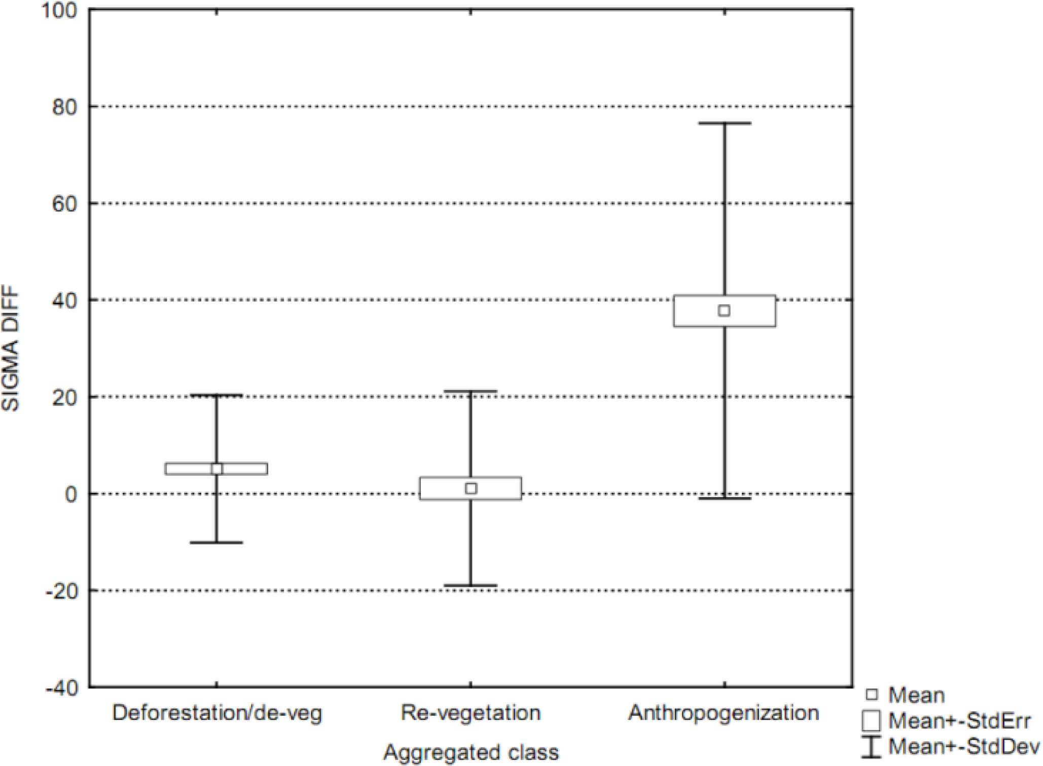
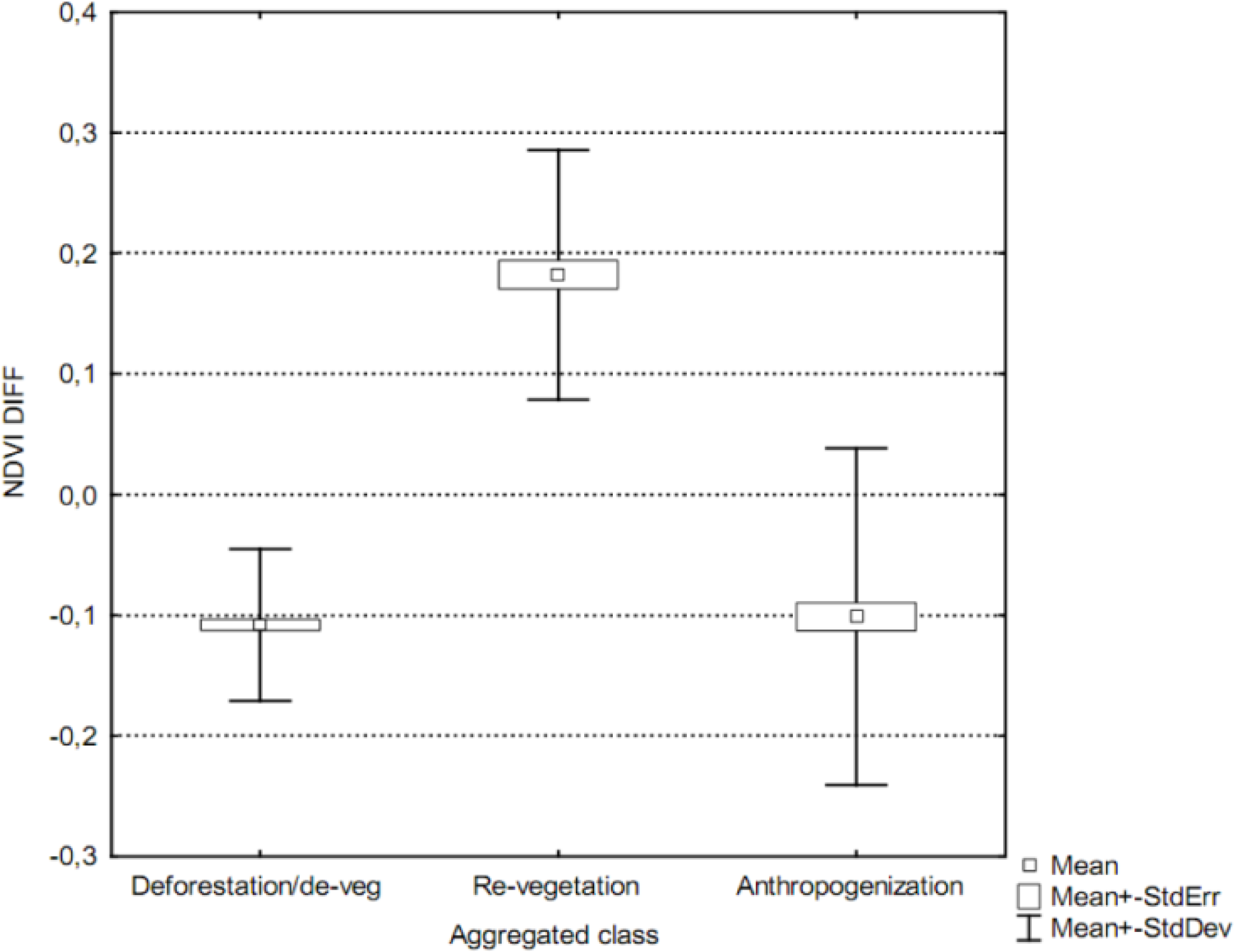
2.2.2. Evaluation of the Spectral Characteristics of Land Cover Changes
- (1)
- Revegetation: transitions of LC, where the amount of vegetation is indicated by the NDVI increase distinctly over time
- (2)
- Devegetation: transitions of LC, where the amount of vegetation is indicated by the NDVI decrease distinctly or disappears entirely over time, but is not connected witch the appearance of new artificial surfaces.
- (3)
- Artificialization: LC transitions connected to the appearance of new artificial surfaces, including buildings, roads and construction sites.
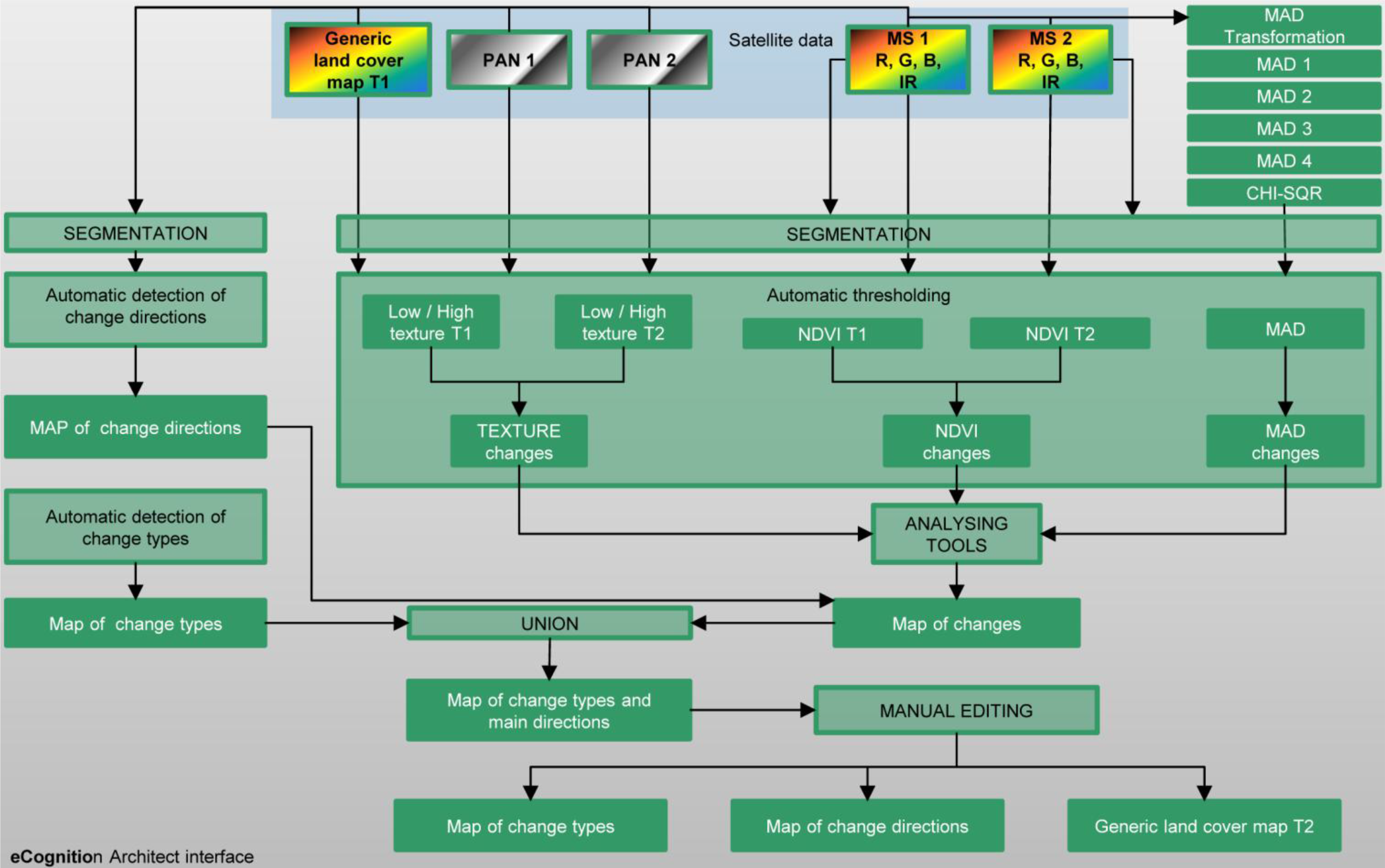
2.2.3. Description of the Algorithm
3. Experimental Section
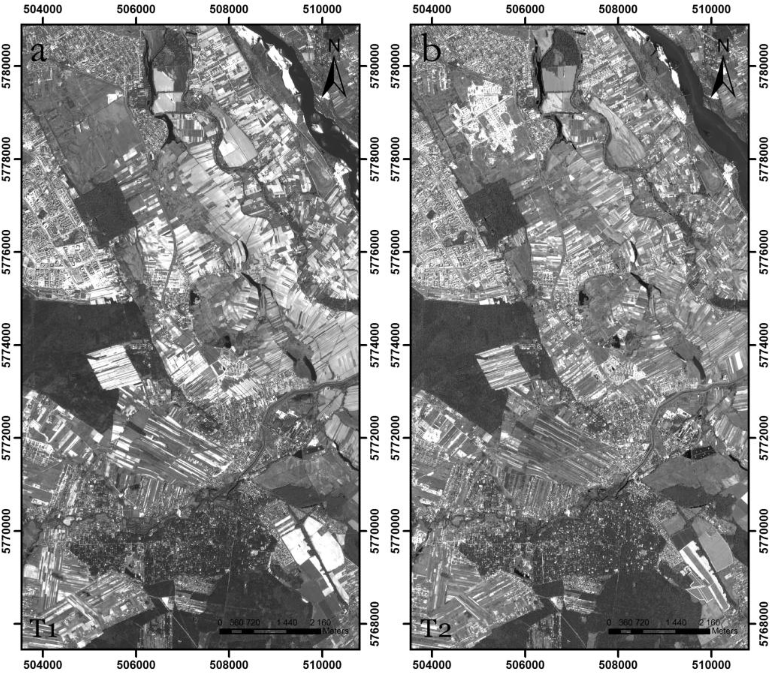
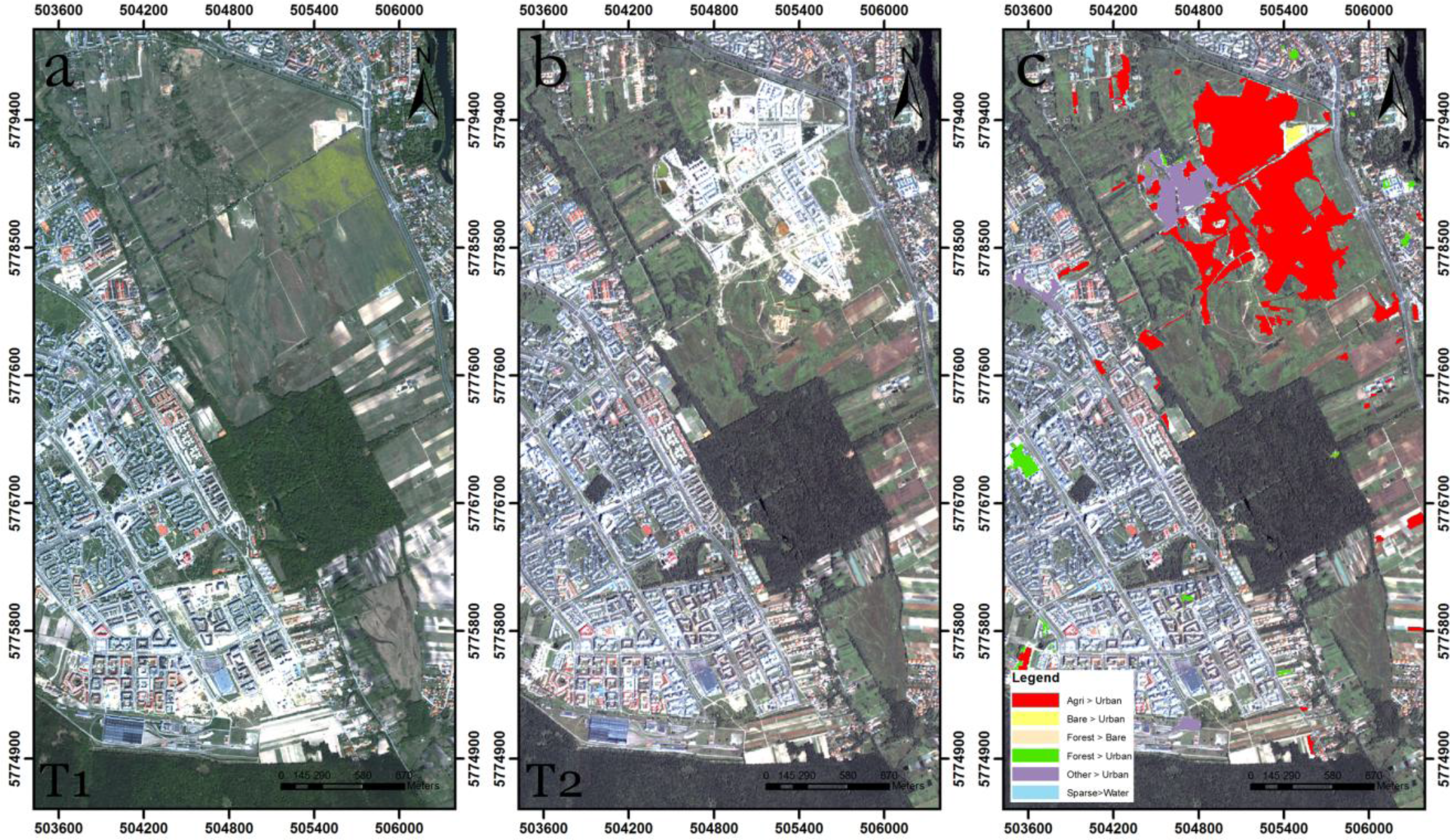
3.1. Warsaw Test Site
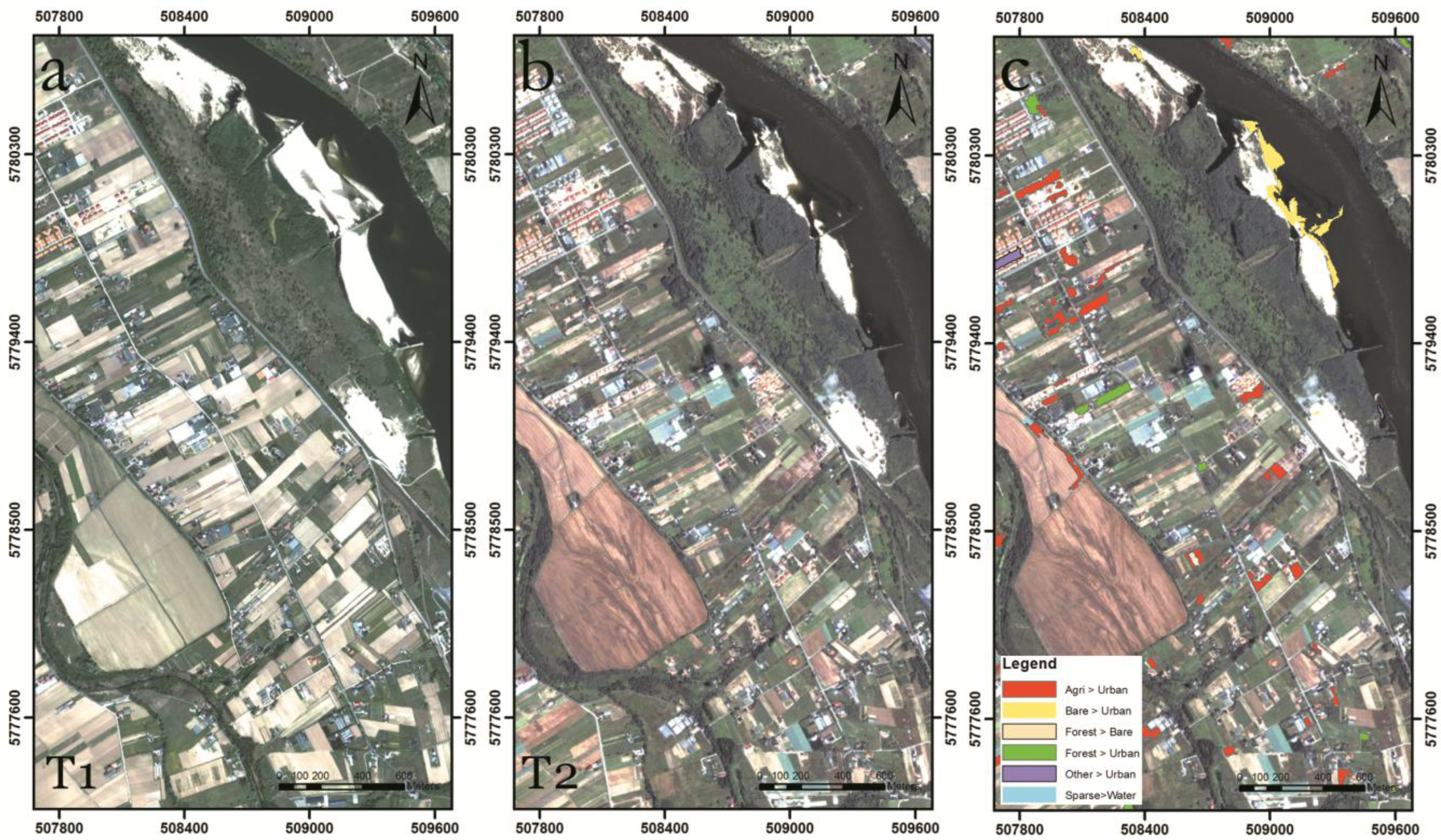
3.2. Results of the Change Detection over the Area Frame Sampling Sites
3.3. Sources of Errors and Uncertainties
4. Conclusions
Acknowledgments
Author Contributions
Conflicts of Interest
References
- Geoland2 Portal. Available online: http://www.geoland2.eu/ (accessed on 14 April 2014).
- Ingram, K.; Knapp, E.; Robinson, J. Change Detection Technique Development for Improved Urbanized Area Delineation; Technical Memorandum CSC/TM-81/6087; Computer Science Corporation: Maryland, MD, USA, 1981. [Google Scholar]
- Jensen, J.R. Introductory Digital Image Processing: A Remote Sensing Perspective; Prentice Hall: Englewood Cliff, NJ, USA, 2005. [Google Scholar]
- Coppin, P.; Jonckheere, I.; Nackaerts, K.; Muys, B.; Lambin, E. Digital change detection methods in ecosystem monitoring: A review. Int. J. Remote Sens 2004, 25, 1565–1596. [Google Scholar]
- Lunetta, R.S.; Knight, J.F.; Ediriwickrema, J.; Lyon, J.G.; Worthy, L.D. Land-cover change detection using multi-temporal MODIS NDVI data. Remote Sens. Environ 2006, 105, 142–154. [Google Scholar]
- Yuan, D.; Elvidge, C. NALC land cover change detection pilot study: Washington DC area experiments. Remote Sens. Environ 1998, 66, 166–178. [Google Scholar]
- Ardila, J.P.; Bijker, W.; Tolpekin, V.A.; Stein, A. Multitemporal change detection of urban trees using localized region-based active contours in VHR images. Remote Sens. Environ 2012, 124, 413–426. [Google Scholar]
- Richards, J.A. Thematic mapping from multitemporal image data using the principal components transformation. Remote Sens. Environ 1984, 16, 35–46. [Google Scholar]
- Coppin, P.R.; Bauer, M.E. Processing of multitemporal Landsat TM imagery to optimize extraction of forest cover change features. IEEE Trans. Geosci. Remote Sens 1994, 32, 918–927. [Google Scholar]
- Qiu, B.; Prinet, V.; Perrier, E.; Monga, O. Multi-Block PCA Method for Image Change Detection. Proceedings of the 12th International Conference on Image Analysis and Processing, Mantova, Italy, 17–19 September 2003; pp. 385–390.
- Nielsen, A.A.; Conradsen, K.; Simpson, J.J. Multivariate Alteration Detection (MAD) and maf postprocessing in multispectral, bitemporal image data: New approaches to change detection studies. Remote Sens. Environ 1998, 64, 1–19. [Google Scholar]
- Blaschke, T.; Hay, G.J.; Kelly, M.; Lang, S.; Hofmann, P.; Addink, E.; Queiroz Feitosa, R.; van der Meer, F.; van der Werff, H.; van Coillie, F.; et al. Geographic object-based image analysis—Towards a new paradigm. ISPRS J. Photogramm. Remote Sens 2014, 87, 180–191. [Google Scholar]
- Blaschke, T.; Burnett, C.; Pekkarinen, A. Image Segmentation Methods for Object-Based Analysis and Classification. In Remote Sensing Image Analysis: Including the Spatial Domain; Springer: Berlin, Germany, 2004; pp. 211–236. [Google Scholar]
- Blaschke, T. Object based image analysis for remote sensing. ISPRS J. Photogramm. Remote Sens 2010, 65, 2–16. [Google Scholar]
- Chen, G.; Hay, G.J.; Carvalho, L.M.T.; Wulder, M.A. Object-based change detection. Int. J. Remote Sens 2012, 33, 4434–4457. [Google Scholar]
- Hussain, M.; Chen, D.; Cheng, A.; Wei, H.; Stanley, D. Change detection from remotely sensed images: From pixel-based to object-based approaches. ISPRS J. Photogramm. Remote Sens 2013, 80, 91–106. [Google Scholar]
- Banaszkiewicz, M.; Smith, G.; Gallego, J.; Aleksandrowicz, S.; Lewinski, S.; Kotarba, A.; Bochenek, Z.; Dabrowska-Zielinska, K.; Turlej, K.; Groom, A.; et al. European Area Frame Sampling Based on Very High Resolution Images. In Land Use and Land Cover Mapping in Europe; Manakos, I., Braun, M., Eds.; Sringer: Berlin, Germany, 2014; pp. 75–88. [Google Scholar]
- Townshend, J.R.G.; Justice, C.O.; Gurney, C.; McManus, J. The impact of misregistration on change detection. IEEE Trans. Geosci. Remote Sens 1992, 30, 1054–1060. [Google Scholar]
- Lewinski, S.; Bochenek, Z.; Turlej, K. Application of an Object-Oriented Method for Classification of VHR Satellite Images Using a Rule-Based Approach and Texture Measures. In Land Use and Land Cover Mapping in Europe; Manakos, I., Braun, M., Eds.; Springer: Berlin, Germany; pp. 193–201.
- De Kok, R.; Wężyk, P. Principles of Full Autonomy in Image Interpretation. The Basic Architectural Design for a Sequential Process with Image Objects. In Object-Based Image Analysis; Blaschke, T., Hay, G.J., Eds.; Springer: Berlin, Germany, 2008; pp. 697–710. [Google Scholar]
- Lewiński, S.; Bochenek, Z.; Turlej, K. Application of object-oriented method for classification of vhr satellite images using rule-based approach and texture measures. Geoinf. Issues 2010, 2, 19–26. [Google Scholar]
- Nielsen, A.A. The regularized iteratively reweighted mad method for change detection in multi- and hyperspectral data. IEEE Trans. Image Process 2007, 16, 463–478. [Google Scholar]
- Canty, M.J. Image Analysis, Classification, and Change Detection in Remote Sensing: With Algorithms for Envi/idl, 2nd ed.; CRC Press: Boca Raton, FL, USA, 2009. [Google Scholar]
- Baatz, M.; Schape, A. Multiresolution Segmentation—An Optimization Approach for High Quality Multi-Scale Image Segmentation Angewandte Geographische Informations Verarbeitung XII. In Angewandte Geographische Informationsverarbeitung XII. Beiträge zum AGIT-Symposium Salzburg 2000; Karlsruhe, Herbert Wichmann Verlag: Berlin, German, 2000; pp. 12–23. [Google Scholar]
- Saba, F.; Valadanzouj, M.; Mokhtarzade, M. The optimazation of multi resolution segmentation of remotely sensed data using genetic alghorithm. Int. Arch. Photogramm. Remote Sens. Spat. Inf. Sci 2013, 1, 345–349. [Google Scholar]
- Johnson, B.; Xie, Z. Unsupervised image segmentation evaluation and refinement using a multi-scale approach. ISPRS J. Photogramm. Remote Sens 2011, 66, 473–483. [Google Scholar]
- Dragut, L.; Tiede, D.; Levick, S.R. Esp: A tool to estimate scale parameter for multiresolution image segmentation of remotely sensed data. Int. J. Geogr. Inf. Sci 2010, 24, 859–871. [Google Scholar]
- Drăguţ, L.; Csillik, O.; Eisank, C.; Tiede, D. Automated parameterisation for multi-scale image segmentation on multiple layers. ISPRS J. Photogramm. Remote Sens 2014, 88, 119–127. [Google Scholar]
- Niemeyer, I.; Bachmann, F.; John, A.; Listner, C.; Marpu, P.R. Object-based change detection and classification. 2009, 7477. [Google Scholar] [CrossRef]
- Im, J.; Jensen, J.R.; Tullis, J.A. Object-based change detection using correlation image analysis and image segmentation. Int. J. Remote Sens 2008, 29, 399–423. [Google Scholar]
- Linke, J.; McDermid, G.; Laskin, D.; McLane, A.; Pape, A.; Cranston, J.; Hall-Beyer, M.; Franklin, S. A disturbance-inventory framework for flexible and reliable landscape monitoring. Photogramm. Eng. Remote Sens 2009, 75, 981–995. [Google Scholar]
- Blaschke, T. Towards a framework for change detection based on image objects. Göttinger Geographische Abhandlungen 2005, 113, 1–9. [Google Scholar]
- Albrecht, F.; Lang, S.; Hölbling, D. Spatial accuracy assessment of object boundaries for object-based image analysis. Int. Arch. Photogramm. Remote Sens. Spat. Inf. Sci 2010, 38, C7. [Google Scholar]
- Foody, G.M. Status of land cover classification accuracy assessment. Remote Sens. Environ 2002, 80, 185–201. [Google Scholar]
- Cohen, J. A coefficient of agreement for nominal scales. Educ. Psychol. Meas 1960, 20, 37–46. [Google Scholar]
- SATChMo Satchmo Change Layers. Available online: http://panufnik.cbk.waw.pl/data/ChangeLayers/ (accessed on 14 April 2014).


| To | Urban/Artificial | Agricultural Areas | Bare Ground | Water | Snow and Ice | Forest/Woodland/Trees | Sparse Woody Vegetation | Grass-land | Other Vegetation | Clouds, Voids, etc. |
|---|---|---|---|---|---|---|---|---|---|---|
| From | ||||||||||
| Urban/artificial | X | 1 | 1 | 1 | 0 | 0 | 0 | 0 | 0 | X |
| Agricultural areas | 2 | X | 2 | 2 | 0 | 0 | 1 | 2 | 1 | X |
| Bare ground | 2 | 2 | X | 2 | 1 | 0 | 1 | 2 | 1 | X |
| Water | 1 | 1 | 2 | X | 1 | 0 | 1 | 2 | 2 | X |
| Snow and Ice | 0 | 0 | 1 | 1 | X | 0 | 0 | 0 | 1 | X |
| Forest/woodland/trees | 2 | 2 | 2 | 2 | 0 | X | 2 | 1 | 1 | X |
| Sparse woody vegetation | 2 | 2 | 2 | 2 | 0 | 2 | X | 2 | 1 | X |
| Grassland | 2 | 2 | 2 | 2 | 0 | 0 | 2 | X | 2 | X |
| Other vegetation | 2 | 2 | 2 | 2 | 1 | 2 | 2 | 2 | X | X |
| Clouds, voids, etc. | X | X | X | X | X | X | X | X | X | X |
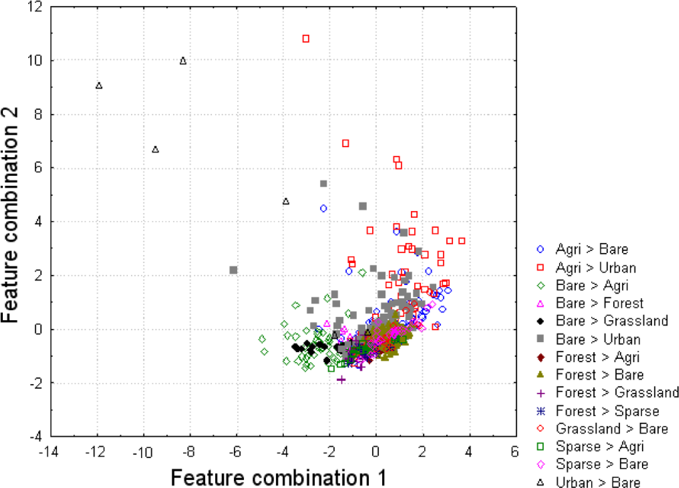
| Type of Land Cover Change | Name of Change Direction |
|---|---|
| Agriculture > urban | Artificialization |
| Bare land > urban | Artificialization |
| Forest > urban | Artificialization |
| Sparse vegetation > urban | Artificialization |
| Agriculture > bare land | Devegetation |
| Forest > agriculture | Devegetation |
| Forest > bare land | Devegetation |
| Grassland > bare land | Devegetation |
| Sparse vegetation > bare land | Devegetation |
| Agriculture > grassland | Revegetation |
| Forest > grassland | Revegetation |
| Sparse vegetation > grassland | Revegetation |
| Urban > agriculture | Revegetation |
| Urban > grassland | Revegetation |
| Classification | ||||
|---|---|---|---|---|
| Change | No Change | Sum | ||
| Reference | Change | 403 | 13 | 416 |
| No change | 97 | 487 | 584 | |
| Sum | 500 | 500 | 1000 | |
| Overall | 0.89 | |||
| Kappa | 0.78 | |||
| Time Span | Total Area (km2) | Change | No Change | Change Direction | Area (km2) | ||
|---|---|---|---|---|---|---|---|
| (km2) | (%) | (km2) | (%) | ||||
| 2009–2010 | 3789.97 | 9.85 | 0.26 | 3780.1 | 99.74 | Devegetation | 8.06 |
| Revegetation | 1.46 | ||||||
| Artificialization | 0.33 | ||||||
| 2010–2011 | 785.01 | 4.41 | 0.56 | 780.59 | 99.44 | Devegetation | 3.57 |
| Revegetation | 0.66 | ||||||
| Artificialization | 0.19 | ||||||
© 2014 by the authors; licensee MDPI, Basel, Switzerland This article is an open access article distributed under the terms and conditions of the Creative Commons Attribution license (http://creativecommons.org/licenses/by/3.0/).
Share and Cite
Aleksandrowicz, S.; Turlej, K.; Lewiński, S.; Bochenek, Z. Change Detection Algorithm for the Production of Land Cover Change Maps over the European Union Countries. Remote Sens. 2014, 6, 5976-5994. https://doi.org/10.3390/rs6075976
Aleksandrowicz S, Turlej K, Lewiński S, Bochenek Z. Change Detection Algorithm for the Production of Land Cover Change Maps over the European Union Countries. Remote Sensing. 2014; 6(7):5976-5994. https://doi.org/10.3390/rs6075976
Chicago/Turabian StyleAleksandrowicz, Sebastian, Konrad Turlej, Stanisław Lewiński, and Zbigniew Bochenek. 2014. "Change Detection Algorithm for the Production of Land Cover Change Maps over the European Union Countries" Remote Sensing 6, no. 7: 5976-5994. https://doi.org/10.3390/rs6075976
APA StyleAleksandrowicz, S., Turlej, K., Lewiński, S., & Bochenek, Z. (2014). Change Detection Algorithm for the Production of Land Cover Change Maps over the European Union Countries. Remote Sensing, 6(7), 5976-5994. https://doi.org/10.3390/rs6075976