Experiments are conducted for each feature extraction method paired together with the aforementioned clustering methods. For the clustering methods, a number of clusters are chosen to be equal to the number of classes, except for the 2D-SOM, where a higher number of clusters is constructed. In the literature, clustering performance evaluation without ground truth is carried out by cluster validation measures, whereas with ground truth information, accuracy calculation after cluster labeling can be used as a performance measure. In 2D-SOM, each cluster is labeled with the majority of the sample labels, whereas in the rest of the methods labeling is carried out by maximizing the overall accuracy in a one-to-one correspondence manner. Kappa values together with the clustering accuracies according to known labels are given as performance measures.
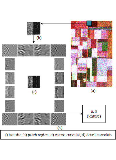
Curvelet subband GD parameter estimation feature extraction is carried out for window size 33 × 33, number of scales 2 and number of orientations 16 (as a result 17 subbands per coherency matrix element). Thus, the number of features per pixel can be given as 204 (17 subbands × 6 elements of coherency matrix × 2 features) for curvelet subband GD parameter estimation. This method is denoted in the tables as μ, σ. It should also be noted that curvelet subband features are normalized feature-wise prior to being fed to clustering methods.
Experimental results are presented in two forms based on clustering accuracies and clustering maps. Clustering accuracies are given according to overall accuracies and Kappa values are able to assess the performance of the proposed feature extraction method compared with standard benchmark features. Clustering accuracies are also further analyzed for higher number of clusters for clustering methods (k-means, FCM, sFCM) that practically use the same number of clusters as class labels. Clustering maps are given in order to be able to provide visual comparison between feature extraction methods on each clustering method.
4.1. Accuracies and Errors
K-means clustering accuracies are given in
Table 1 for the average of 20 runs for each feature extraction method. The best clustering accuracy is achieved for SRAD features with
k-means algorithm up to 65.41% with the experiments.
FCM clustering overall accuracies are given in
Table 2 for the average of 20 runs. It can be seen from
Table 2 that clustering overall accuracies can be increased compared to hard membership
k-means, with the introduction of fuzzy cluster memberships. It should also be noted that as the
m value increases, the threshold constraint is met at a small number of iterations. Feature extraction methods can be ordered with respect to clustering accuracies as SRAD, μ, σ features, original data and H/A/α for FCM method.
sFCM clustering method results are calculated for a fixed fuzzy membership value (
m = 2), various feature-space and spatial fuzzy membership values (
p,
q ∈ {0,1,2,4,8}) and different window sizes (
w ∈ {5,11,21}). sFCM results of the 20-run averages for best clustering accuracy yielding parameters are given in
Table 3. Compared to
k-means and FCM, it can be said that the introduction of spatial information through clustering iterations with sFCM, enhanced clustering accuracy for H/A/α more than the curvelet subband μ, σ features. The best clustering accuracy for sFCM is achieved by SRAD features up to 85.11%.
2D-SOM clustering results are calculated for 7 × 7, 9 × 9, 11 × 11 and 13 × 13-sized hexagonal grid networks and 3, 4, 5 and 6 initial neighborings respectively. 2D-SOMs run for 1000 iterations and resulting clusters are labeled as the majority label they contain. In
Table 4, overall clustering accuracies are given together with the number of unique labels assigned in parenthesis. SRAD features with 7 × 7 and 9 × 9 SOM networks have better clustering accuracies compared to μ, σ features, whereas as the network grows μ, σ features presents better accuracies. It can be inferred from the results in
Table 4 that SRAD extracts similar features and curvelet subband GD parameter estimation extracts discriminating features. Thus with SRAD as the network grows, 2D-SOM cannot set previously clustered together samples apart clearly. On the other hand, with μ, σ features, as the network grows and the number of clusters increases, the use of discriminating features results in labeled samples falling into similar clusters.
The confusion matrices results from 2D-SOM with 13 × 13 topology for SRAD and curvelet subband μ, σ features are given in
Tables 5 and
6, respectively.
The most confused labels and the number of confusions for SRAD with 13 × 13 2D-SOM can be listed as (label1–label2: sum of # of mislabeled samples): 2–7:864 (670 + 194), 2–6:205, 3–8:192, 5–6:177. The most confused labels and the number of confusions for curvelet subband μ, σ features with 13 × 13 2D-SOM can be listed as (label1–label2: sum of # of mislabeled samples): 2–7:393, 3–7:182, 1–2:96. The most mislabeling occurs with labels 2 (grass) and 7 (lucerne), which can be considered alike by means of vegetation structure and therefore by SAR backscattering mechanism. This result can also be seen in 2D-SOM spatial node labels, where almost the only neighbors for Lucerne-labeled clusters are grass-labeled clusters.
Kappa values for the best clustering accuracies are given in
Table 7. Kappa value can be considered as differentiation from the expected value of random labeling accuracies and is given as
Equation (28), where
P(
a) is the confusion matrix accuracy probability and
P(
e) is the probability of random labeling. Overall the best Kappa value as 0.9382 is reached with the use of μ, σ features in 13 × 13 topology 2D-SOM. SRAD features again with 13 × 13 topology-SOM are placed second with Kappa value 0.9009.
Overall evaluation of feature extraction methods on
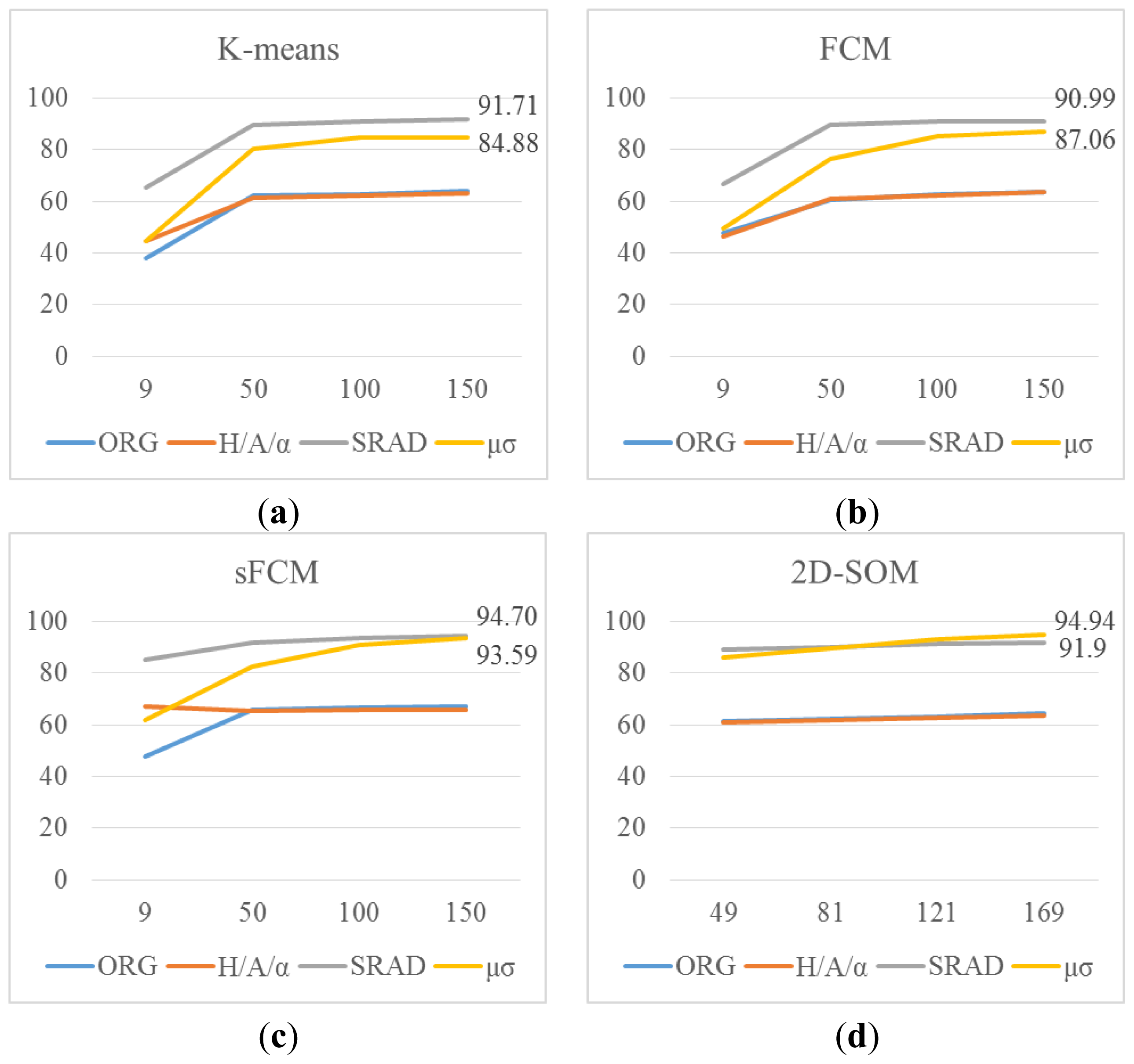
k-means, FCM and sFCM together with 2D-SOM is also carried out with higher number of clusters for 20 runs. That is
k-means, FCM, sFCM are evaluated with 50, 100 and 150 clusters and labels are given the same way as in 2D-SOM. FCM is run for
m = 2, sFCM is run for
m = 2,
p = 1,
q = 1 and
w = 21. The results are given in graphical form with x-axis showing number of clusters and y-axis showing accuracies as in
Figure 5.
It can be seen from the graphs in
Figure 5 that curvelet subband μ, σ features starts with slightly lower accuracy compared to SRAD in all clustering methods; however, with the increasing number of clusters curvelet subband μ, σ features reach up to the SRAD accuracies. In 2D-SOM clustering curvelet subband μ, σ features gives even better accuracies compared to SRAD. The sFCM method is also run with 169 clusters for SRAD and curvelet subband μ, σ features, and accuracies of 94.82% and 94.67% are obtained respectively. The best accuracy overall is obtained by 13 × 13 2D-SOM with curvelet subband μ, σ features with 94.94%. These results are also consistent with nine cluster results of
k-means, FCM and sFCM.
Practically, feature extraction in SAR images is conducted following a speckle noise reduction step. However, the proposed feature extraction method can be carried out without speckle reduction, as it utilizes spatial features naturally by curvelet transform. Moreover as the curvelet subband features are extracted on averages and standard deviations the disturbing effect of speckle noise can be eliminated to some extent. Results from
Table 1–
Table 4 and graphs from
Figure 5 suggest that the proposed method is as accurate as SRAD features or even better at some experimental setups thereby demonstrating that the proposed method is robust against speckle noise.
4.2. Clustering Maps
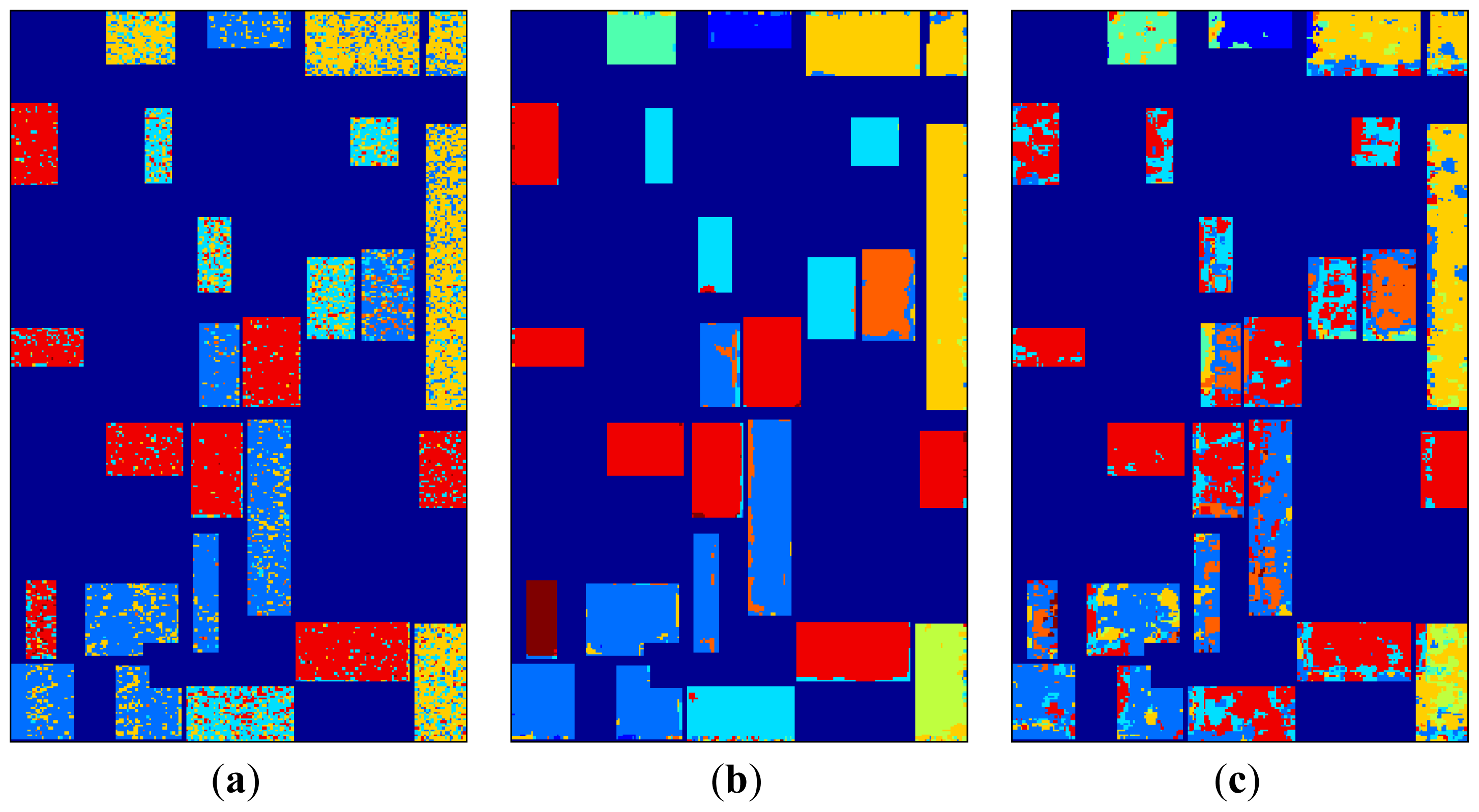
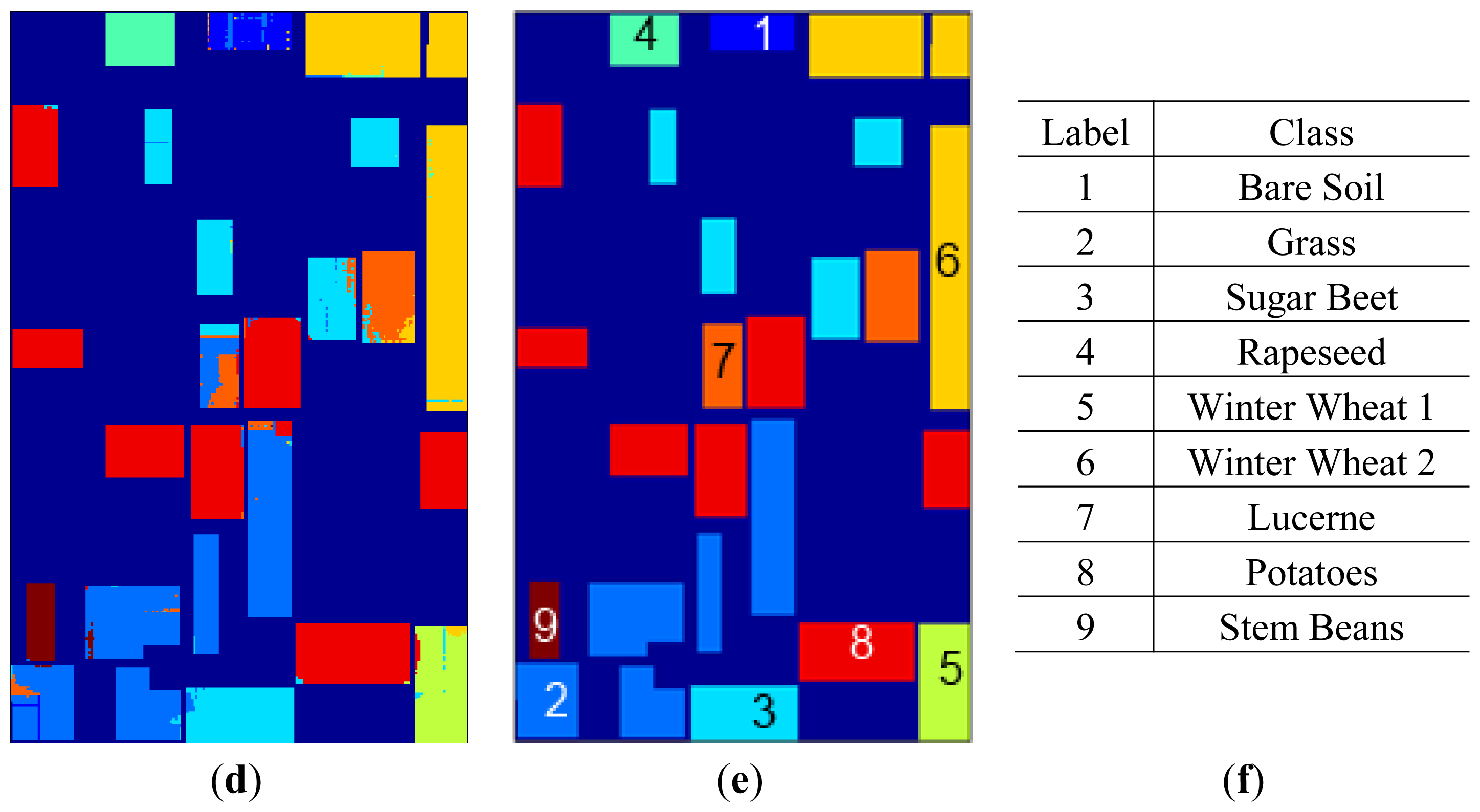
K-means clustering maps are given in
Figure 6 together with labels and the label map. Using only feature space hard memberships and similarity measures to cluster centers,
k-means clustering mappings result in cluttered small regions for original data and H/A/α, whereas bigger homogeneous regions can be seen for SRAD and μ, σ features where spatial information is diffused through feature extraction.
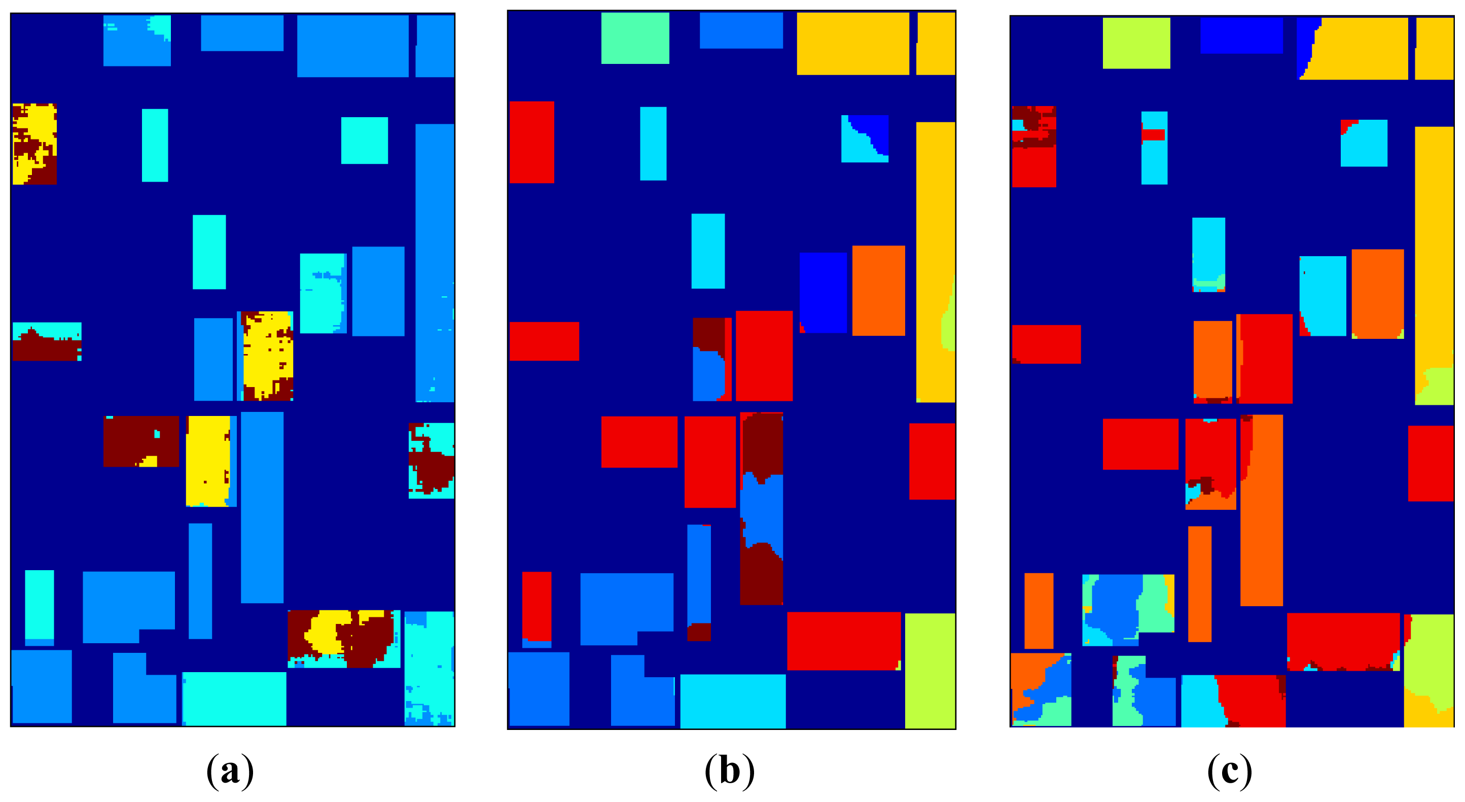
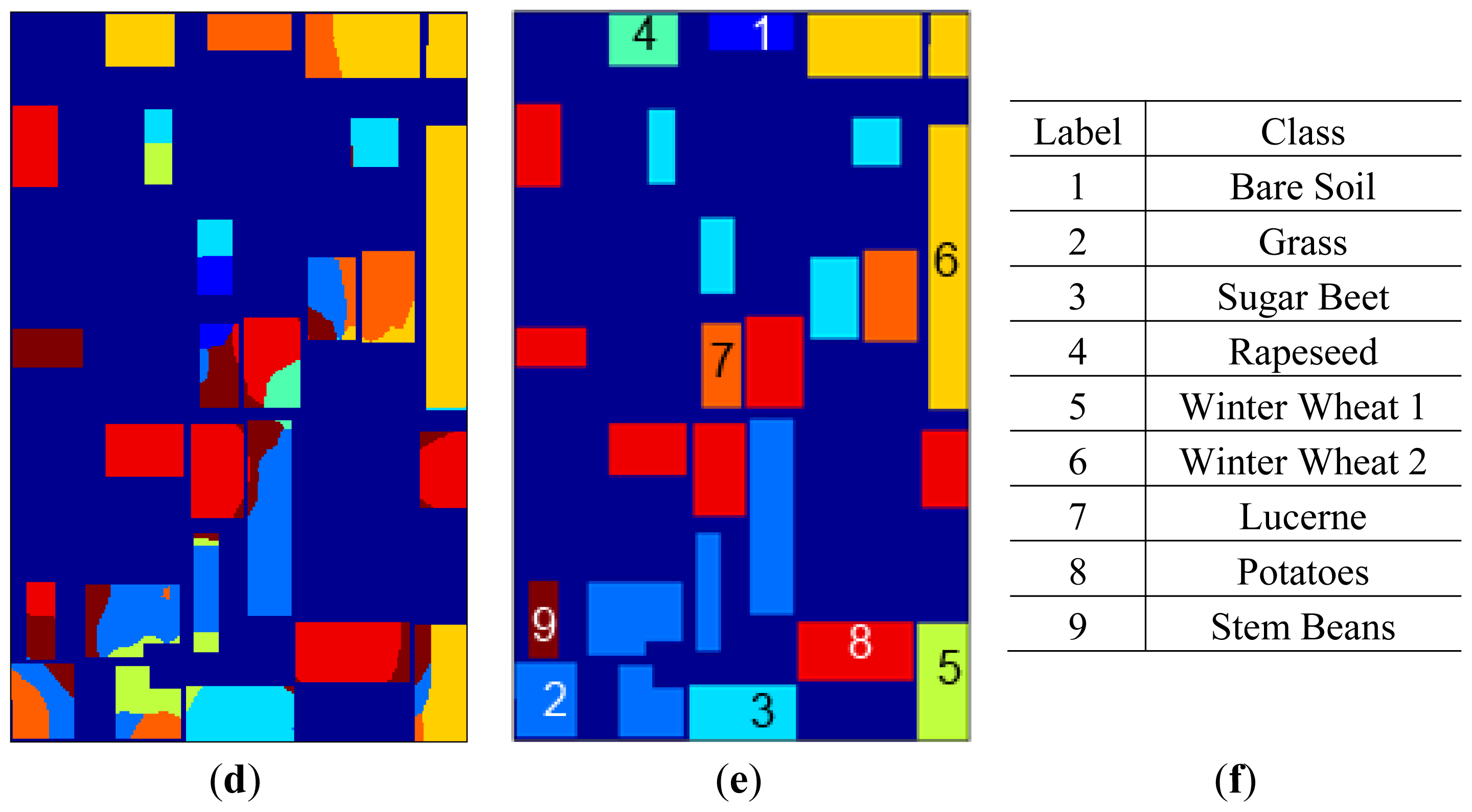
FCM clustering maps for the best clustering accuracy yielding
m values are given in
Figure 7 together with labels and the label map. In
Figure 7, clustering maps are given for original data with
m = 16, SRAD with
m = 1.2, H/A/α features with
m = 16 and curvelet subband GD μ, σ parameter estimation features with
m = 1.4.
sFCM clustering maps for the best clustering accuracy yielding parameters are given in
Figure 8 together with labels and the label map. Apart from spatial information being diffused by feature extraction in SRAD and curvelet μ, σ features, the introduction of spatial information through sFCM clustering steps also enables bigger homogeneous-labeled regions for all feature extraction methods.
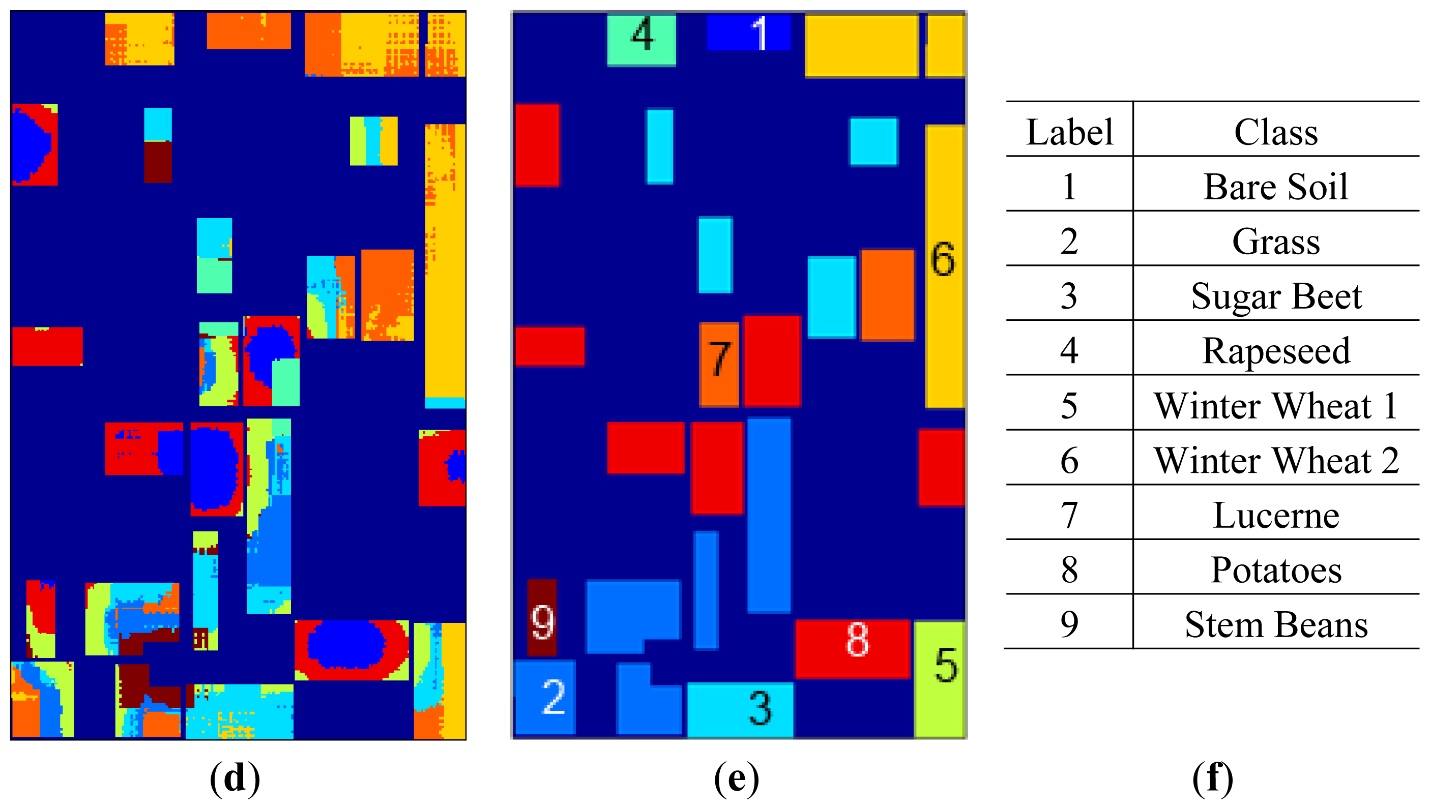
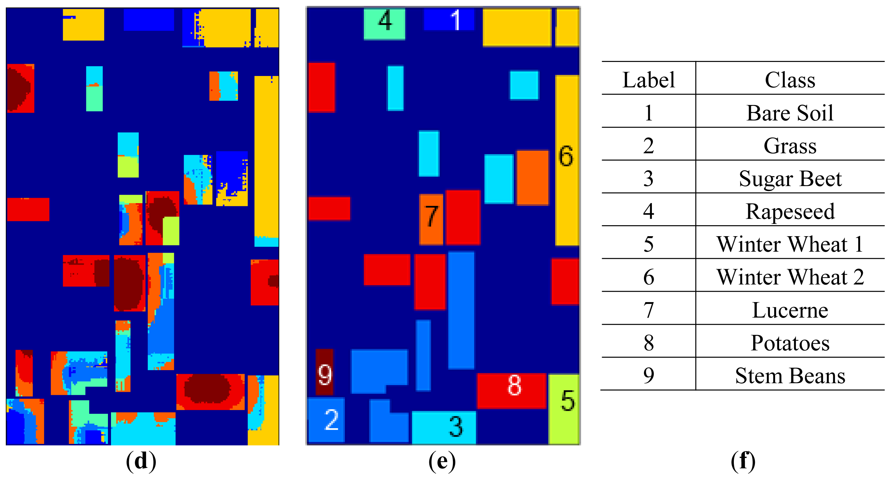
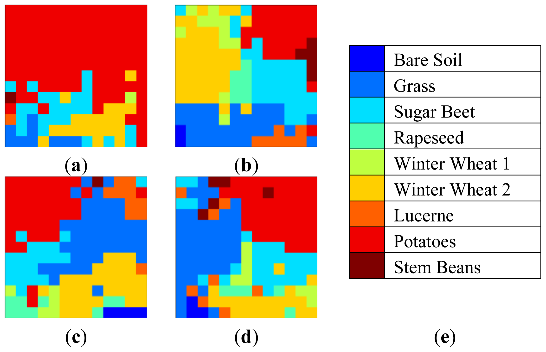
2D-SOM classification maps for 13 × 13 topologies are given in
Figure 9. In analyzing 2D-SOM cluster mapping for SRAD, it can be seen that confusions in the labeling mostly occur at edges of the regions. This situation can be explained with SRAD preserving edges by definition. Cluster confusion can also be seen due to feature diffusion in neighboring regions both in SRAD and μ, σ features.
2D-SOM nodes labeled as their majority labels are given in
Figure 10 for 13 × 13 topology with consistent coloring from cluster mappings. This figure illustrates 2D-SOM node label neighborhood and gives insight for cluster label confusion.


