Article

FAO-56 Dual Model Combined with Multi-Sensor Remote Sensing for Regional Evapotranspiration Estimations

1
CESBIO/UMR 5126, 18 av. Edouard Belin, bpi 2801, 31401 Toulouse Cedex 9, France
2
GREF, Université de Carthage/INAT, 43, Avenue Charles Nicolle 1082-Tunis-Mahrajène, Tunisia
3
CNRM-GAME, Météo-France, CNRS, URA 1357, 42 avenue Gaspard Coriolis, 31057 Toulouse Cedex 1, France
*
Author to whom correspondence should be addressed.
Remote Sens. 2014, 6(6), 5387-5406; https://doi.org/10.3390/rs6065387
Submission received: 27 January 2014 / Revised: 3 June 2014 / Accepted: 4 June 2014 / Published: 11 June 2014
(This article belongs to the Special Issue Earth Observation for Water Resource Management in Africa)

Abstract

:
The main goal of this study is to evaluate the potential of the FAO-56 dual technique for the estimation of regional evapotranspiration (ET) and its constituent components (crop transpiration and soil evaporation), for two classes of vegetation (olives trees and cereals) in the semi-arid region of the Kairouan plain in central Tunisia. The proposed approach combines the FAO-56 technique with remote sensing (optical and microwave), not only for vegetation characterization, as proposed in other studies but also for the estimation of soil evaporation, through the use of satellite moisture products. Since it is difficult to use ground flux measurements to validate remotely sensed data at regional scales, comparisons were made with the land surface model ISBA-A-gs which is a physical SVAT (Soil–Vegetation–Atmosphere Transfer) model, an operational tool developed by Météo-France. It is thus shown that good results can be obtained with this relatively simple approach, based on the FAO-56 technique combined with remote sensing, to retrieve temporal variations of ET. The approach proposed for the daily mapping of evapotranspiration at 1 km resolution is approved in two steps, for the period between 1991 and 2007. In an initial step, the ISBA-A-gs soil moisture outputs are compared with ERS/WSC products. Then, the output of the FAO-56 technique is compared with the output generated by the SVAT ISBA-A-gs model.

1. Introduction

In semi-arid regions, and the Mediterranean basin in particular, agricultural productivity and water resources regularly suffer from serious crises, as a consequence of limited levels of precipitation, combined with the occurrence of long periods of drought, which are typical features of the Mediterranean climate [1]. In this context, the accurate monitoring of vegetation cover and hydric stress can be a valuable tool, especially for areas which rely on rainfed agriculture in water-limited environments. A second challenge for the well-adapted management of this agriculture is to accurately determine the level of evapotranspiration, in order to quantify the soil water stock. In recent years, a variety of physical surface models have been proposed at regional and global scales [2]. The most accurate of these are the SVAT models [36].
On the other hand, the initial FAO-56 model is the most commonly used and practical approach for the estimation of crop water requirements and local scale evapotranspiration [7], and is based on a simple combination of a reference evapotranspiration value (ET0) and crop coefficients. The FAO-56 dual model distinguishes between the respective contributions of plant transpiration (Kcb) and soil evaporation (Ke) [8]. In recent years, various attempts have been made to combine the latter model with remote sensing data for operational applications [914]. These studies were motivated, in particular, by the need to retrieve vegetation cover dynamics from vegetation indices derived from optical satellite observations [9,10,15,16]. Most applications of this model are related to the study of irrigated areas, for the effective planning and use of irrigation water.
In recent years, sustained scientific activity based on the interpretation of remotely sensed data has made it possible to develop various methodologies for the characterization of the spatio-temporal variability of continental surface parameters (vegetation characteristics and soil moisture), on both local and global scales. In the case of vegetation cover, various indices based on the use of optical data have been proposed for the retrieval of vegetation characteristics (e.g., leaf area index, vegetation fraction, NDVI (Normalized Difference Vegetation Index), etc.). The NDVI is the most commonly used index, and is expressed by the ratio: NDVI = (RNIR − RRED)/(RNIR + RRED), where RNIR is the near-infrared (NIR) reflectance and RRED is the red reflectance. This index is sensitive to the presence of green vegetation [17,18], and has been used in various studies dealing with the estimation of the potential photosynthetic activity of vegetation [10,1922]. As a consequence of its formulation, the NDVI is able to robustly characterize green vegetation, despite varying atmospheric conditions in the red and NIR bands [23,24]. Nevertheless, in the case of high levels of vegetation density, the NDVI can suffer from saturation effects [25], which bias the estimated levels of evapotranspiration. In semi-arid regions, this behavior is rarely observed. Several different methodologies based on the interpretation of microwave sensor data have also been developed for the determination of soil moisture [2631]. A large number of studies have demonstrated the potential of low-resolution spaceborne (active microwave) scatterometers for land surface characterization, in particular for the estimation of soil moisture [3237].
In this context, the aim of the present study is to illustrate the ability of the FAO-56 dual approach to estimate evapotranspiration at regional scales, without making use of complex physical surface models requiring large quantities of input data. In an initial step, the effectiveness of the FAO-56 dual approach, which is commonly used for irrigation management [9,10], is evaluated. Then, the combination of this model with data generated by remote sensing is considered, not only for the study of vegetation as proposed in other studies [912,14], but also for the purposes of soil moisture analysis. Under such conditions, the spatio-temporal variations of these two fundamental parameters can be taken into account in the transpiration and evaporation estimations.
In Section 2, the studied site and the remotely sensed and ground databases are presented. In Section 3, the FAO dual model is introduced, and the concurrent use of remotely sensed data is discussed. In Section 4, the proposed approach is compared with the outputs of a physical SVAT model: the ISBA-A-gs. Finally, the authors’ conclusions are presented in Section 5.

2. Database and Processing
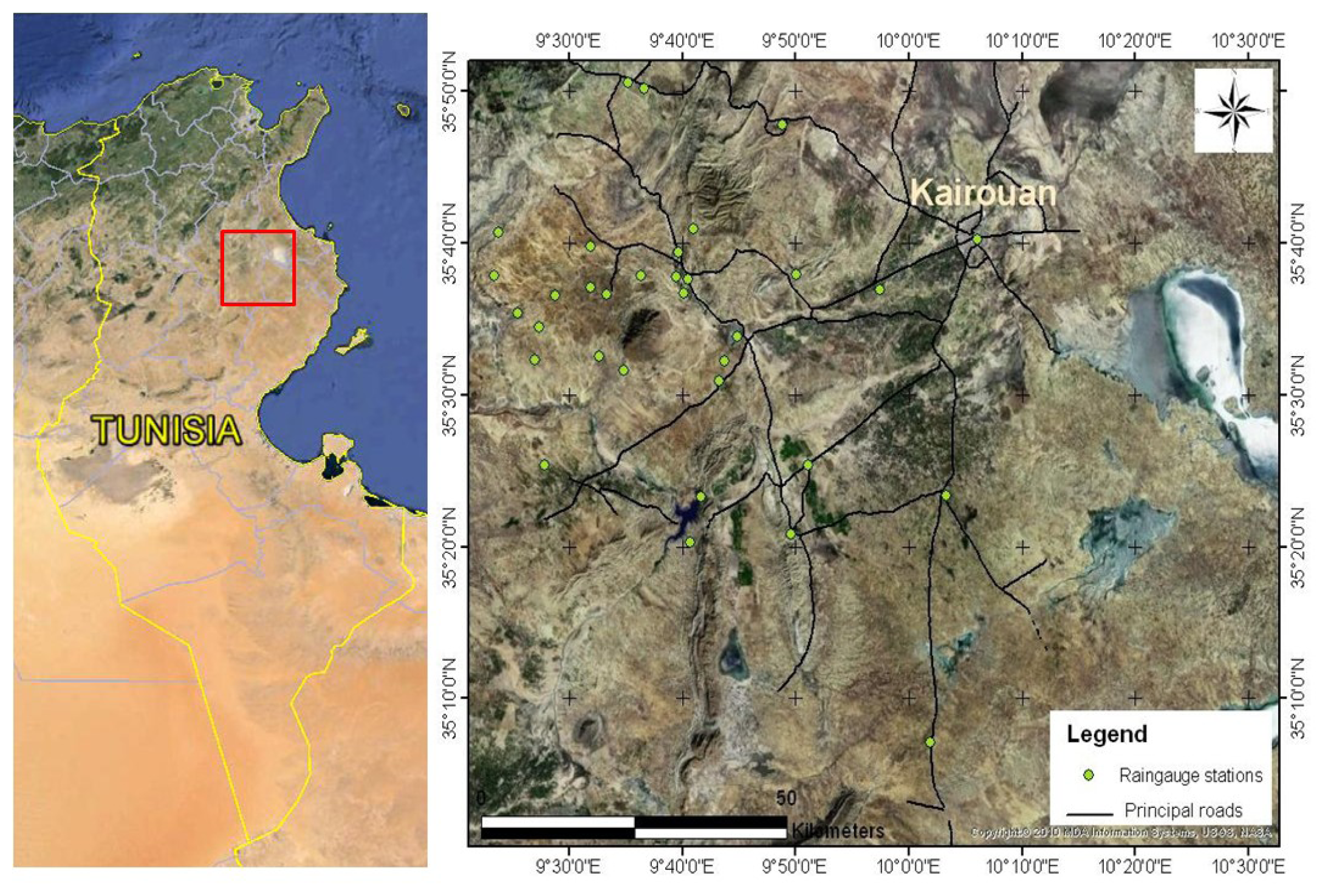
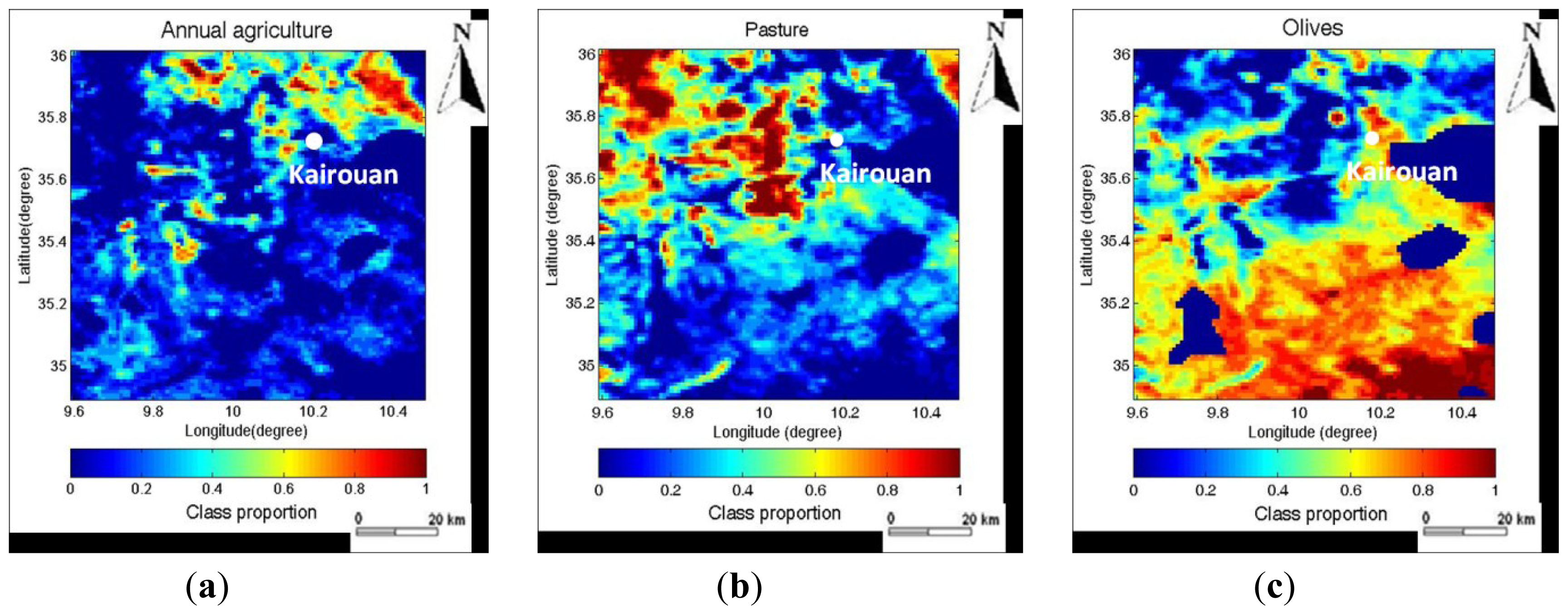
2.1. Studied Site

The studied site is the Kairouan plain, which is situated in central Tunisia (35°–35°45′N; 9°30′–10°15′E) (Figure 1) and is characterized by a semi-arid climate [38]. The average annual rainfall is approximately 300 mm per year, with a rainy season lasting from October to May. The rainfall patterns in this semi-arid area are highly variable in time and space. The mean daily temperature in Kairouan City ranges between a minimum of 10.7 °C in January and a maximum of 28.6 °C in August, with a mean value equal to 19.2 °C. The mean annual potential evapotranspiration (Penman) is close to 1600 mm. The landscape has no relief and land use is dominated by agriculture, with two main types of vegetation cover: annual agriculture and olive trees. A ground campaign carried out over more than 20 test fields revealed that the mean soil texture is composed of 45% sand, 32% clay and 23% loam. Sandy soils are more commonly observed in the areas characterized by olive tree cultivation.

2.2. Satellite Products

2.2.1. ERS/WSC Moisture Products

The scatterometers carried by ESA’s dual ERS satellites (launched in 1991 and 1995, the dual ERS satellite mission was finally decommissioned in September 2011) are operated in the C-band (5.3 GHz) in the vertical polarization. Over land, the measured radar backscatter coefficient is sensitive to surface parameters (soil moisture, surface roughness, vegetation characteristics) and the emission characteristics of the radar (incidence angle, polarization and frequency). A change detection approach developed by the Institute of Photogrammetry and Remote Sensing (IPF), Vienna University of Technology (TU-Wien), has been applied to the estimation of soil moisture, based on radar measurements [31,32,39,40]. The proposed moisture products have been validated in different regions of the globe, such as the Canadian Prairies [32], the Iberian Peninsula [35], Western Africa [34,41], France [37] and Australia [42]. The TU-Wien algorithm is based on scaling of the normalized backscattering coefficient to a value corresponding to a 40° incidence angle, lying between the lowest value which occurs during the driest conditions, and the highest value which occurs during the wettest conditions. The retrieved moisture index, referred to as the “surface soil moisture” (SSM), can range between 0% and 100% and represents the water content present in the first 5 cm of soil. Based on the interpretation of cells approximately 50 × 50 km in size, the TU-Wien products have a grid spacing of 25 km, and a temporal resolution of approximately two to three measurements per week. In order to compare SSM values with ground measurements on the same study site [43] or modeled surface moisture values, these products were converted to physical units of m3·m−3, using the method described by Pellarin et al. [36]. The TU-Wien Soil Water Index (SWI), which provides the water content along a 1 m deep profile, is derived from the SSM values measured on different successive dates. These products have already been validated and used in various hydrological studies [29,3537,44]. Amri et al. [43] discussed the validation of ERS and ASCAT products, through the use of continuous thetaprobe recordings of ground soil moisture in the Kairouan plain. These authors revealed a strong correlation between the ground measurements recorded between 2010 and 2011, and satellite products corresponding to the same period, with an RMSE (the root mean square error) equal to 0.06 cm3/cm3 for surface moisture and 0.039 cm3/cm3 for the SWI.

2.2.2. SPOT-VGT NDVI Products

The 10-day synthesis (S10) products derived from SPOT-VGT (SPOT-VEGETATION) data are available at full resolution (1 km), and include 10-day NDVI data [45]. For these products, top-of-atmosphere corrections were applied using the SMAC (Simplified Method for Atmospheric Corrections) algorithm [46], which corrects for molecular and aerosol scattering, water vapor, ozone and other gas absorption effects. The parameters taken into account in the atmospheric corrections are the aerosol optical depth (AOD), the atmospheric water vapor and ozone, and a Digital Elevation Model used for atmospheric pressure estimation [47]. The water vapor parameter is obtained once every six hours from Météo-France with a 1.5° × 1.5° grid cell resolution. Although the AOD is currently retrieved from B0 data (blue spectral band of SPOT-VGT, 0.43–0.47 μM), combined with the NDVI [47], prior to 2001 it was a static data set which varied as a function of latitude only. Different systematic errors (misregistration of the different channels, calibration of the linear array detectors for each spectral band) are corrected in the final P product, which is re-sampled to a Plate carrée geographic projection. The S10 products are available [48].

2.3. Ground Measurements

2.3.1. Precipitation Data

Precipitation estimations were based on a network of 30 rain gauges, distributed over the entire site (Figure 1). The Inverse Distance Weighting (IDW) interpolation algorithm was used to derive daily precipitation maps. This algorithm estimates values at non-sampled points, by computing the weighted average of data observed at nearby points [49,50]. The landscape is mainly flat in the validation areas, and there is no mountainous terrain able to influence the spatial distribution of rainfall. The precipitation time series and the NDVI data set are thus available with a spatial resolution of 1 km.

2.3.2. Meteorological Data

Meteorological data, including air temperature, humidity, wind speed, net radiation and rainfall measurements, have been recorded over the last 20 years by an automatic weather station located in the Kairouan Plain. Daily averaged climatic parameters were computed in order to determine the daily reference evapotranspiration ET0 (mm/day), in accordance with the FAO-56 Penman-Monteith parameterization [51].
The global radiation was determined from Météosat data [52] retrieved from the SoDa server (Solar radiation Databases for environment [53]), established by the Mines ParisTech graduate school. In this database, global radiation data is available from January 1985 to December 2005, at temporal intervals of one day and a spatial resolution of 20 km.

2.4. Land Use Mapping

Low spatial resolution SPOT Vegetation NDVI images were used to map the land into three characteristic classes: olive trees, annual agriculture and pastures. It is important to note that these classes were labeled: “Olive trees”, “Annual Agriculture” corresponding to cereals and “Pastures”. Later, for the purposes of estimating regional evapotranspiration, only two principal classes were considered: Olive trees and annual agriculture.
In recent years, several approaches have focused on the disaggregation of low resolution mixed pixels in different land cover classes [54]. A linear mixing theory is generally used, in which it is assumed that the reflectance (respectively NDVI) of a mixed pixel is given by the sum of the mean reflectance (respectively NDVI) values of the different land cover classes within the pixel, weighted by their corresponding fractional cover. The identification of typical NDVI profiles, representative of each of these land cover classes, is the first step in the disaggregation methodology. These pixels are identified by making use of information related to the class composition of each pixel, retrieved from a high-resolution land-cover map.
The general expression is given by Equation (1), and the RMS of this quantity is given by Equation (2):
Y i ( t ) = j = 1 p π ij × ρ j ( t ) + ɛ i ( t )
R M S E i = 1 T × t = 1 T ( ɛ i ( t ) )
where: Yi(t) is the average signal observed at pixel i and time t, and is estimated from the NDVI time series produced by SPOT-VGT; πij is the area occupied by the jth class in the ith pixel: the unknown term in Equation (1); ρj(t) is the signal assigned to the jth class at time t, and is calculated for each class (pure pixels are considered) from the NDVI time series produced by SPOT-VGT; ɛi is the error term; p is the number of classes, T is the number of observations, i is the pixel index, and j is the class index.
The error term defined in Equation (2) is the square of the differences between the NDVI signature assigned to each class, and the NDVI profile observed in the ith pixel.
Disaggregation techniques are designed to estimate the proportion (between 0 and 1) of specific classes occurring within each pixel. The result is a certain number of fraction images, each corresponding to the relevant land-cover class. While this information describes the composition of the class, it does not provide any indication as to how the classes are spatially distributed within the pixel. The outcome is thus quite different from that obtained with conventional classification algorithms, in which a single “crisp” land cover map, containing all classes, is produced. Figure 2 shows a land-use map for two classes. The pixels having low proportions (dark blue areas) for all 3 classes of land use correspond to areas covered by water (sebkhas, dams). These areas are masked in all of the maps used in the following analysis.

3. Proposed Approach for the Retrieval of Evapotranspiration

3.1. Description of the Basic FAO-56 Model

The algorithm used in the present study is based on the FAO-56 dual crop coefficient model developed by [7], which describes the relationship between crop evapotranspiration under non-standard conditions (ET) and a reference level of evapotranspiration (ET0). The crop coefficient (Kc) is separated into two components: the basal crop coefficient (Kcb) and the soil water evaporation coefficient (Ke):
E T = ( K s · K c b + K e ) * E T 0
where ET0 is estimated at 24 h intervals using the FAO Penman-Monteith equation [7]; Kcb: the basal crop coefficient, KS is the stress coefficient and Ke: the soil water evaporation coefficient.
The daily reference evapotranspiration ET0 is determined with a spatial resolution of 20 km, allowing ET0 maps to be derived at daily intervals, for each growing season (from September of one year to August of the following year), with the same resolution as the SoDa data. The cumulative annual ET0 values are consistent with the observed levels of ET in this region (approximately 1600 mm/year).

3.2. Application with a Dual Vegetation Cover

In the present study, two types of vegetation cover are considered for each pixel: cereals (annual agriculture) and olive trees. For each pixel, the evapotranspiration ET under non-standard conditions is estimated using:
E T = [ F r c e r e a l s [ ( f c - c K c b - c K s + ( 1 - f c - c ) K e ) ] + F r o l i v e [ ( f c - o K c b - o K s + ( 1 - f c - o ) K e ) ] ] * E T 0
where: fc is the fractional cover; Fr is the cover percentage per pixel, for each class, KS is the stress coefficient and the indices “o” and “c” denote the cereal and olive tree classes, respectively.
The parameters (Kcb and Ke) used in Equation (4) are derived from the remotely sensed SPOT-VGT NDVI index, and ERS/WSC soil moisture products, respectively.
Ks describes the effect of water stress on crop transpiration.
K s = T A W - D r ( 1 - p ) T A W
  • Dr: root zone depletion (mm). The equation number 86 of the FAO No. 56 guidelines [7] is used to calculate this parameter.
  • TAW: Total available soil water in the root zone (mm), estimated using the equation number 82 of the FAO No. 56 guidelines [7].
  • p: fraction of TAW that a crop can extract from the root zone without suffering water stress. This parameter is derived for each class from table 22 of the FAO No. 56 guidelines [7].

3.2.1. Computing the Values of Kcb and fc

Further details of the proposed annual agriculture (cereals) estimations can be found in Er-raki et al. [9]. The calibrations made at the Tensift site in Morocco Er-raki et al. [9] were also applied to the studied site, due to their similarities in terms of climate and cereal yields.
Kcb is defined as:
K c b = 1.07 × [ 1 - ( N D V I - N D V I min N D V I max - N D V I min ) 0.84 0.54 ]
where NDVImin and NDVImax are the minimum and maximum values of the NDVI associated with bare soil and dense vegetation, respectively. The values retrieved from the SPOT-VGT NDVI index time series, used in the present study, are 0.1 and 0.6.
fc is the vegetation cover fraction defined by Er-raki et al. [9]:
f c = 1.18 * ( N D V I - N D V I min )
In the case of olive trees, the crop coefficients proposed in the FAO Bulletin No. 56 [7] for the estimation of the water requirements of olive trees are not applicable to the present case study, due to the low percentage of coverage corresponding to this culture. In a recent study, Testi, et al. [55] established a relationship between the ET and the cover fraction, which is used to determine the value of Kcb applicable in the present study.
In the case of olive trees, a tree spacing of approximately 20 m and a tree diameter of approximately 4 m area were considered. This leads to a value of fc value equal to 8%.

3.2.2. Computation of the Parameter Ke

In recent years, various different approaches have been proposed to relate soil resistance to soil moisture [5658]. Chanzy and Bruckler [57] proposed an empirical method relating soil evaporation to soil moisture and climate demand, for different types of soil texture. In arid and semi-arid regions, the soil evaporation which occurs after a rainfall event is a process of major importance, whenever the local agriculture is characterized by a low density vegetation cover. When this term is determined accurately, it allows a reliable estimation to be made of the stock of water available for use by the vegetation. In this section, a simple approach is used for the estimation of soil evaporation, which is equal to the ET0 whenever the surface layer is saturated. A method developed by Merlin et al. [58] was used, allowing soil evaporation to be related to the surface soil moisture (0–5 cm) estimated from radar satellite measurements. The parameter Ke can then be written as:
K e = [ 1 2 - 1 2 · cos ( π · θ L / θ max ) ] P For  θ L θ max
where θL is the soil water content in the soil layer of thickness L, θmax is the soil moisture at saturation, and P is a parameter given by the following expression:
P = ( 1 2 + A 3 L - L 1 L 1 ) L E p B 3
In this expression, L1 is the thinnest layer of soil represented (here 0–5 cm), and A3 (unit-less) and B3 (W·m−2) are a priori the two best-fit parameters, which depend on the soil’s texture and structure.
θmax was estimated from continuous ground thetaprobe measurements, acquired over a period of three years.
θL was considered to be equal to the remotely sensed surface soil moisture products produced by the ERS and ASCAT scatterometers. As described above, these products were converted to physical units of m3·m−3, using the method described by Pellarin et al. [36].
Soil evaporation is assumed to reach its maximum value in the case of saturated soils, with a value defined as being equal to ET0, which is close to zero for very dry surfaces.

3.3. Description of the ISBA Model Used to Evaluate the FAO Dual Approach

Since it would not be realistic to use local flux measurements made at the field scale to validate the FAO-56 dual approach for applications involving low spatial resolution data (0.5° × 0.5°, i.e., regional scale), the validation used in the present study was based on comparisons made with the operational ISBA model developed by Météo France. This model uses the force-restore method proposed by Deardoff [59] to compute the corresponding variations in soil surface energy and water budget [5]. The model uses three layers to represent the soil’s hydrology: the upper surface layer, the root-zone layer and the deep soil layer [60], and water interception storage and snow pack variations are also taken into account [61]. Within each grid, the heterogeneity of infiltration, precipitation, topography and vegetation are accounted for, and the conversion of precipitation into runoff over saturated surfaces is based on the TOPMODE approach [62,63]. Within each grid cell, the heterogeneity of land cover and soil depths is taken into account through the use of a tile approach, in which the cell is divided into a series of sub-grid patches. For each tile in a grid cell, distinct energy and water budgets are calculated. The multiplicative model developed by Jarvis [64] is used to determine the stomatal resistance of the vegetation. ISBA-A-gs is a variant of the ISBA model [5], which takes photosynthesis and its coupling with leaf-level stomatal conductance into account, and in which a biochemical soil–vegetation–atmosphere transfer representation is used to model the diurnal cycle of photosynthesis [65]. Then, the canopy conductance to water vapor is computed by integrating the photosynthesis model over the vegetation canopy, using a one-dimensional radiative transfer model within the vegetation. The canopy conductance is then used in the original ISBA model [66] to calculate plant transpiration. The other components of evapotranspiration (soil evaporation and evaporation of intercepted rain) are simulated in the same manner as in the original ISBA model. In addition to meteorological variables and surface temperature, soil evaporation depends on surface soil moisture and the vegetation coverage fraction. The interception reservoir is assumed to evaporate at the potential rate and depends on the LAI and the vegetation coverage fraction. The ECOCLIMAP look-up tables are used to generate the LAI (Leaf Area Index) inputs used by the ISBA model. ISBA-A-gs also implements a new representation for soil moisture stress, in which two different drought responses can be applied: one is used for herbaceous vegetation [67], and the other for forests [68].

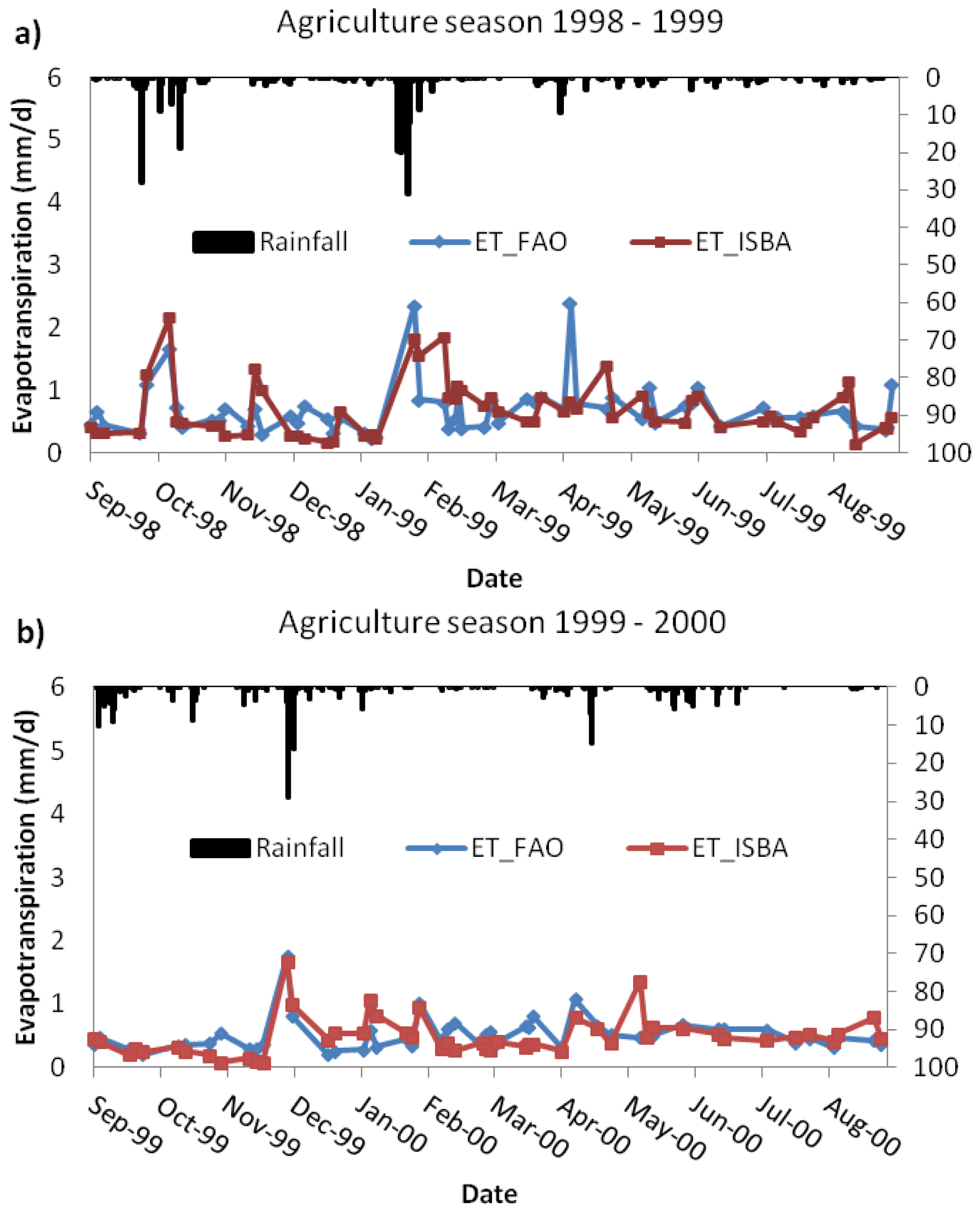
4. ISBA-A-gs Model Inter-Comparison with the FAO-56 Approach

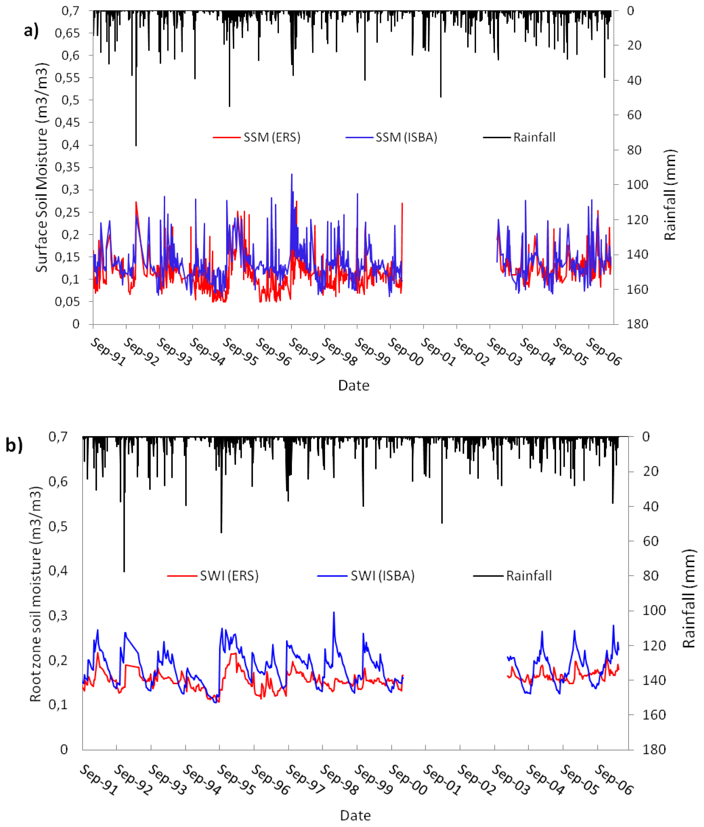
4.1. Analysis of the ISBA-A-gs Soil Moisture Output

In Figure 3, the ERS/WSC soil moistures, validated by Amri et al. [43] over the studied site and described in Section 2.2, are compared with the output generated by the ISBA model, and are plotted together with the precipitation time series. Three statistical parameters: RMSE (the root mean square error), R2 (the coefficient of determination), and the bias are used to compare the ERS and ISBA datasets.
The satellite data products are compared with two ISBA-A-gs outputs; the modeled top layer (the first five centimeters of soil) and the soil moisture profiles (down to a depth of 100 cm), for the 16-year period from 1991–2007. It should be noted that the ERS measurements and the corresponding remotely sensed moisture products are not available for the period from 2001–2003. As can be seen in Figure 3a, local variations in the ERS surface moisture products are not completely retrieved by the ISBA outputs. In fact, the latter corresponds to the first 10 centimeters of soil, which are less strongly influenced by atmospheric conditions (rain, wind and solar radiation) than the first five centimeters of soil, which affect the ERS/WSC radar measurements. Despite the strong heterogeneity of the moisture profile in the first centimeters, the statistics of the resulting comparison are good: RMSE = 0.04 m3·m−3, bias = 0.02, and R2 = 0.52.
In Figure 3b, the monthly SWI ISBA-A-gs outputs (0.5 m depth) are compared with the ERS estimations, showing that these two products have a good degree of coherence. In general, a delay of several days is observed between significant rainfall events and the corresponding increase in water soil content, determined using the ERS measurements.
The statistics of the compared data are good: RMSE equal to 0.03 m3·m−3, R2 = 0.5, and a low bias equal to 0.008. A change in behavior can be observed in 1997: before this date, less than one data point (determined using the ERS1 scatterometer only) was available per week, from which the algorithm could be developed. After 1997, the ERS1 and ERS2 scatterometers were both able to provide a combined two to three data points per week, for use in the SWI estimations, and there is thus a difference in the product’s accuracy between these two periods. Although the SWI itself is not used in the evaporation estimation, comparisons made with this product are used to validate the ISBA-A-gs model over the studied site.

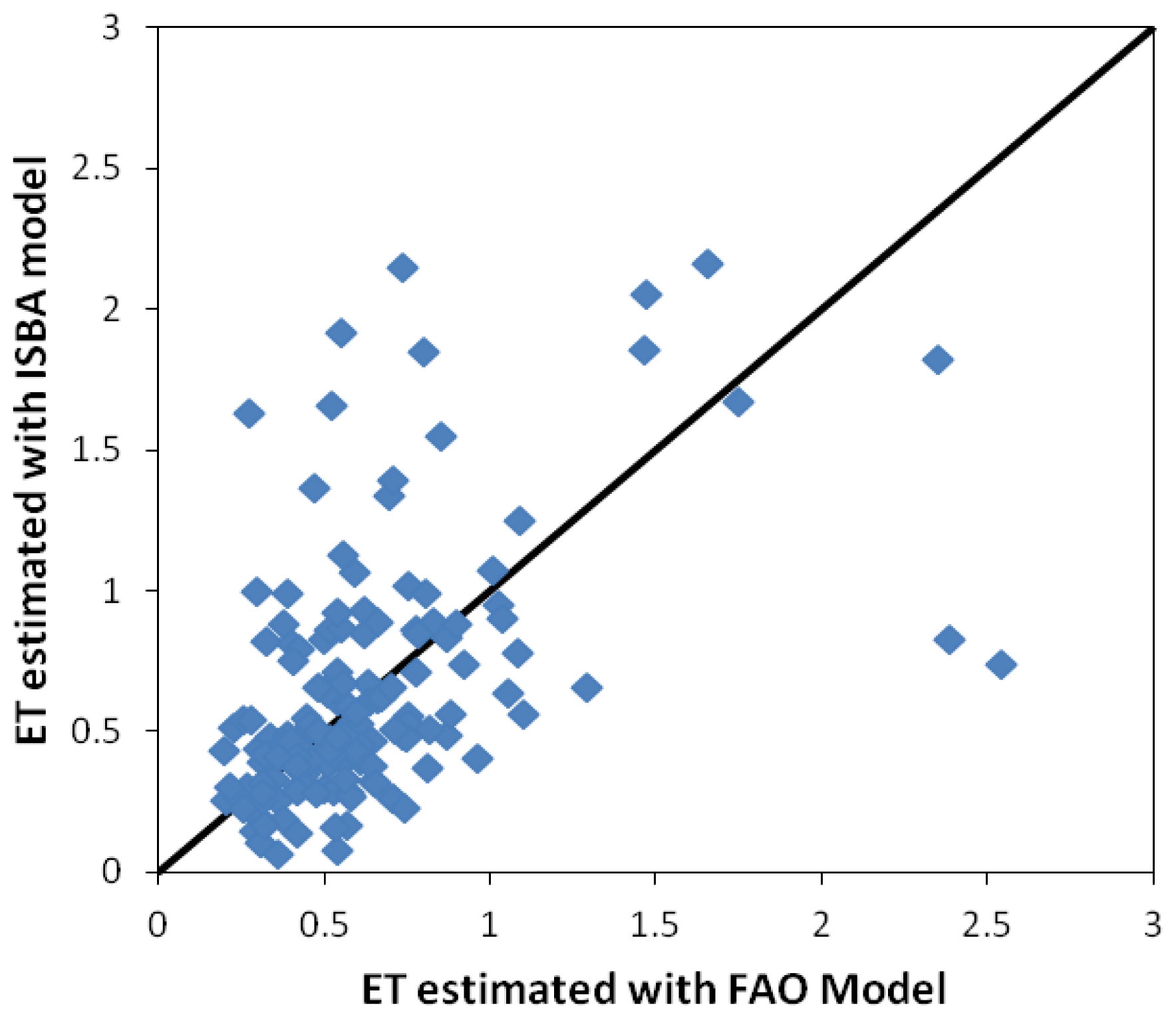
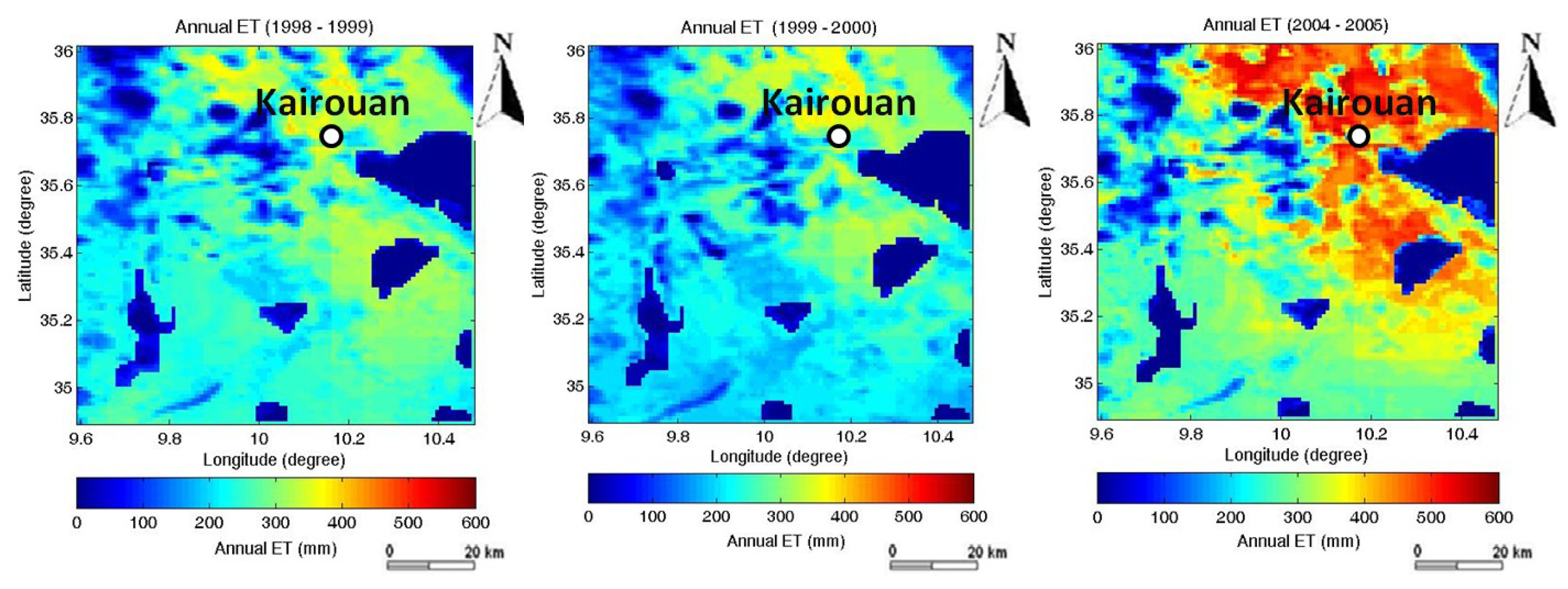
4.2. Inter-Comparison between ISBA-A-gs and FAO-56 Approaches

Figure 4 compares the ISBA and FAO model evapotranspiration simulations over the studied area, for a single ISBA pixel with a spatial resolution corresponding to 0.5° in latitude and 0.5° in longitude, for the periods between 1998 and 2000 and between 2004 and 2005. These two products are compared only on dates for which ERS/WSC-based determinations of the Ke evaporation parameter are available. The two products are found to be in good agreement, and the statistical parameters derived from the FAO simulation are reasonable: RMSE = 0.36 mm/day, with a correlation R2 = 0.55. The discrepancies observed at some points in this figure are related, in particular, to the soil evaporation component, and to the occurrence (or not) of a precipitation event: all of the data points characterized by a strong discrepancy between the two models involve a precipitation event, which was taken into account by one of the models, but not the other. This is mainly due to the input used in the ISBA-Ags model. In the case of the present study, the ISBA model was driven by the ERA-Interim atmospheric forcing, corresponding to the ERA-Interim global ECMWF atmospheric reanalysis, projected onto a 0.5° grid. Since precipitation is underestimated by the latter product [69], the monthly Global Precipitation Climatology Centre (GPCC) precipitation product was used to correct the precipitation bias in the 3-hourly ERA-Interim estimates [70]. The availability of a smaller number of GPCC precipitation observations for northern Africa, than for Europe, thus provides an explanation for the reduced robustness of the Tunisian precipitation series. The retrieved levels of FAO approach are in coherency with other studies realized over other semi-arid regions [9,71].
The FAO model values for the ISBA pixel (0.5° × 0.5°) correspond to the mean value of 1 km pixel estimations. In order to evaluate the scale effect, the FAO model is computed directly at the ISBA pixel scale, by considering the mean NDVI values at this scale, for vegetation fractions and Kcb estimations, and for two types of vegetation cover (olive trees and cereals). The intercomparison between FAO model levels, calculated at two different scales, reveals an rms error of 0.2 mm/day and a correlation coefficient equal to 0.85, for the period (1991–2007). This result indicates that the FAO dual model has only a limited scaling effect.
Figure 5a compares the ET simulated by the ISBA-A-gs model with that predicted by the FAO-56 model, for the 1998–1999 agricultural season during which the total precipitation was approximately 280 mm. A good degree of consistency is observed for the results obtained with these two models. However, on some dates, large differences are observed between FAO-56 estimates and ISBA-A-gs outputs, probably as a consequence of the rainfall events taken into account in the ISBA-A-gs model. The statistical parameters derived from the simulation are reasonable: RMSE equal to 0.39 mm/day, correlation strength given by R2 = 0.55, and a low bias equal to 0.009 mm/day.
The second example, illustrated in Figure 5b, corresponds to the 1999–2000 agricultural season, characterized by a relatively dry growing season and a total annual precipitation of approximately 250 mm. During this season, the results given by the two models are found to be more consistent. The FAO-56 model retrieves almost the same trends as the ISBA-A-gs model, for both high and low values of ET. The statistical parameters from the comparison are good: RMSE = 0.25 mm/day, correlation strength R2 = 0.61, and a low bias equal to 0.01. This comparison shows that the models are more consistent during the driest period of the season (from June to August). This is mainly due to the very limited number of rainfall events at this time of the year. Under these conditions, it is easier for the FAO dual model to retrieve the evaporation dynamics corresponding to small temporal variations in moisture, caused for example by a single rainfall event during a period of drought.
For both of these agricultural seasons, the two models are found to be well correlated with the rainfall events, with a clear increase in the level of evapotranspiration following strong precipitation events. However, some distinct inconsistencies can be observed between the two simulations. As an example, the FAO-56 model retrieves a high level of ET, due to a 10 mm precipitation event in April 1999, which was not detected by the ISBA-A-gs simulations. Conversely, in May 2000, a rise in the level of ET is predicted by the ISBA-A-gs model, whereas this is not predicted by the FAO-56 model. Prior to the May 2000 peak observed in the ISBA-A-gs model, one small (1 mm) rainfall event occurred, which probably had a very small influence on the real level of ET. It is thus likely that the discrepancy observed between the two models results from an exaggeration of this event, at the precipitation input of the ISBA-A-gs model.
Finally, the cumulative seasonal water requirement maps for the 1998–1999, 1999–2000 and 2004–2005 agricultural seasons, estimated by the FAO-56 dual crop coefficient model combined with satellite data, are shown in Figure 6. It should be noted that these maps are well matched with the land-use maps. As an example, during the 1998–1999 agricultural season the water requirements were slightly greater for annual crops (400 mm) than for olive trees (200 mm). The very low ET areas generally correspond to olive trees with a low vegetation cover fraction, as can be seen in Figure 2. All of the areas covered by water (dams, sebkhas) were masked, and were not taken into account in the ET calculations.
By comparing the water requirements of annual crops with the average annual rainfall in the Kairouan plain (300 mm), an initial estimation is made of the hydric deficit, which should be offset through the use of irrigation.

5. Conclusions

The FAO-56 dual approach, which is commonly used for irrigation management, is applied to the simulation of evapotranspiration at the regional scale. This is combined with remotely sensed, multi-sensor data. Two main types of vegetation cover, cereals and olive trees, are considered in this analysis. The vegetation fractions represented by these two classes of vegetation are retrieved by means of a multi-temporal classification of SPOT-VGT time series images. The evapotranspiration is computed over the studied area for two vegetation classes, weighted by their respective vegetation fractions.
The cereal crop coefficient and vegetation fraction estimations are based on NDVI SPOT-VGT data, through the use of an empirical relationship. Soil evaporation is estimated by a simple approach developed by Merlin, et al. [58] established between this quantity and surface soil moisture, using ERS/WSC radar products developed by the TU-Wien. Saturated soils are associated with the highest level of evaporation, and the driest soils have approximately zero evaporation.
The ISBA-A-gs SVAT model is compared to the FAO approach, using simulations covering the period between 1991 and 2007. The ISBA soil moisture outputs are validated using ERS/WSC products developed by the TU-Wien. A good degree of coherence is observed for surface moisture, with an RMSE equal to 0.04 m3·m−3, R2 equal to 0.52 and a bias equal to 0.002. The soil moisture profiles are also in good agreement, with an RMSE equal to 0.03 m3·m−3, R2 equal to 0.5, and a bias equal to 0.008. When the ISBA and FAO models are compared for the same study area, they are found to be strongly coherent. In the case of daily comparisons, an RMSE equal to 0.36 mm/day is found, which is low by comparison with the mean ET values, estimated at approximately 2 mm/day. The soil moisture profiles are well correlated, with R2 equal to 0.5. These results illustrate the strong potential of this simple approach, in which the FAO-56 model is combined with several satellite observations (optical and microwaves), to retrieve evapotranspiration levels particularly in semi-arid regions.

Acknowledgments

This study was funded by two sources: the French national MISTRALS program, and the ANR AMETHYST “ANR-12-TMED-0006-01”. The authors extend their thanks to VITO for kindly providing them with its SPOT-VEGETATION NDVI products, and to the ISIS program for providing them with the SPOT images used in this study. They would also like to thank the Tunisian Ministry of Agriculture for providing the precipitation data used in this study, as well as the technical teams of the IRD, INAT, CTV-Chebika and INGC for their strong collaboration and support with the implementation of ground-truth measurements.

Conflicts of Interest

The authors declare no conflict of interest.
  • Author ContributionsRim Amri and Mehrez Zribi proposed modifications and application of FAO-56 model and discussions of results. Gilles Boulet helps on analysis and interpretation of the use of FAO-56 model. Zohra Lili-Chabaane participates to ground measurements and analysis of correlation between results and the site climate. Camille Szczypta and Jean-Christophe Calvet proposed simulations of ISBA-A-gs model and participate to interpretation of comparison between FAO-56 and ISBA-Ags.

References

  1. Amri, R.; Zribi, M.; Lili-Chabaane, Z.; Duchemin, B.; Gruhier, C.; Chehbouni, A. Analysis of vegetation behavior in a north African semi-arid region, using SPOT-Vegetation NDVI data. Remote Sens 2011, 3, 2568–2590. [Google Scholar]
  2. Mueller, B.; Hirschi, M.; Jimenez, C.; Ciais, P.; Dirmeyer, P.A.; Dolman, A.J.; Fisher, J.B.; Jung, M.; Ludwig, F.; Maignan, F.; et al. Benchmark products for land evapotranspiration: LandFlux-EVAL multi-data set synthesis. Hydrol. Earth Syst. Sci 2013, 17, 3707–3720. [Google Scholar]
  3. Braud, I.; Dantas Antonio, A.C.; Vauclin, M.; Thony, J.L.; Ruelle, P. A. Simple Soil Plant Atmosphere Transfer Model (SisPAT): Development and field verification. J. Hydrol 1995, 166, 213–250. [Google Scholar]
  4. Mahfouf, J.-F.; Manzi, O.; Noilhan, J.; Giordani, H.; Déqué, M. The land surface scheme ISBA within the Météo-France climate model ARPEGE. Part I: Implementation and preliminary results. J. Clim 1995, 8, 2039–2057. [Google Scholar]
  5. Calvet, J.C.; Noilhan, J.; Roujean, J.L.; Bessemoulin, P.; Cabelguenne, M.; Alioso, A.; Wigneron, J.P. An interactive vegetation SVAT model tested against data from six contrasting sites. Agric. For. Meteorol 1998, 92, 92–95. [Google Scholar]
  6. Saux-Picart, S.; Ottlé, C.; Perrier, A.; Decharme, B.; Coudert, B.; Zribi, M.; Boulain, N.; Cappelaere, B.; Ramier, D. SEtHyS_Savannah: A multiple source land surface model applied to sahelian landscapes. Agric. For. Meteorol 2009, 149, 1421–143. [Google Scholar]
  7. Allen, R.G.; Pereira, L.S.; Raes, D.; Smith, M. Chapter 5. In Crop Evapotranspiration-Guidelines for Computing Crop Water Requirements, Irrigation and Drain; Paper No. 56; Food and Agriculture Organization: Rome, Italy, 1998; p. 300. [Google Scholar]
  8. Allen, R.G. Using the FAO-56 dual crop coefficient method over an irrigated region as part of an evapotranspiration intercomparison study. J. Hydrol 2000, 229, 27–41. [Google Scholar]
  9. Er-Raki, S.; Chehbouni, G.; Guemouria, N.; Duchemin, B.; Ezzahar, J.; Hadria, R. Combining FAO-56 model and ground-based remote sensing to estimate water consumptions of wheat crops in a semi-arid region. Agric. Water Manag 2007, 87, 41–54. [Google Scholar]
  10. Er-Raki, S.; Chehbouni, A.; Boulet, G.; Williams, D.G. Using the dual approach of FAO-56 for partitioning ET into soil and plant components for olive orchards in a semi-arid region. Agric. Water Manag 2010, 97, 1769–1778. [Google Scholar] [Green Version]
  11. Belaqziz, S.; Khabba, S.; Er-Raki, S.; Jarlan, L.; le Page, M.; Kharrou, M.H.; El Adnani, M.; Chehbouni, A. A new irrigation priority index based on remote sensing data for assessing the networks irrigation scheduling. Agric. Water Manag 2013, 119, 1–9. [Google Scholar]
  12. Campos, I.; Villodre, J.; Carrara, A.; Calera, A. Remote sensing-based soil water balance to estimate Mediterranean holm oak savanna (dehesa) evapotranspiration under water stress conditions. J. Hydrol 2013, 494, 1–9. [Google Scholar]
  13. Conrad, M.; Rahmann, M.; Machwitz, M.; Stulina, G.; Paeth, H.; Dech, S. Satellite based calculation of spatially distributed crop water requirements for cotton and wheat cultivation in Fergana Valley, Uzbekistan. Glob. Planet. Chang 2013, 110, 88–98. [Google Scholar]
  14. Mateos, L.; González-Dugo, M.P.; Testi, L.; Villalobos, F.J. Monitoring evapotranspiration of irrigated crops using crop coefficients derived from time series of satellite images. I. Method validation. Agric. Water Manag 2013, 125, 81–91. [Google Scholar]
  15. González-Piqueras, J. Crop Evapotranspiration by Means of Remote Sensing Determination of the Crop Coefficient. Regional Scale Application: 08-29 Mancha Oriental Aquifer; Universitat de València: Valencia, Spain, 2006. [Google Scholar]
  16. Purevdorj, T.; Tateishi, R.; Ishiyama, T.; Honda, Y. Relationships between percent vegetation cover and vegetation indices. Int. J. Remote Sens 1998, 19, 3519–3535. [Google Scholar]
  17. Sellers, P.J. Canopy reflectance, photosynthesis and transpiration. Int. J. Remote Sens 1985, 6, 1335–1372. [Google Scholar]
  18. Deblonde, G.; Cihlar, J. A multiyear analysis of the relationship between surface environmental variables and NDVI over the Canadian landmass. Remote Sens. Rev 1993, 7, 151–177. [Google Scholar]
  19. Delbart, N.; Kergoat, L.; Toan, T.L.; Lhermitte, J.; Picard, G. Determination of phenological dates in boreal regions using normalized difference water index. Remote Sens. Environ 2005, 97, 26–38. [Google Scholar]
  20. Myneni, R.B.; Los, S.O.; Asrar, G. Potential gross primary productivity of terrestrial vegetation from 1982 to 1990. Geophyis. Res. Lett 1995, 22, 2617–2620. [Google Scholar]
  21. Propastin, P.; Kappas, M. Modeling net ecosystem exchange for grassland in Central Kazakhstan by combining remote sensing and field data. Remote Sens 2009, 1, 159–183. [Google Scholar]
  22. Laurila, H.; Karjalainen, M.; Kleemola, J.; Hyyppä, J. Cereal yield modeling in Finland using optical and radar remote sensing. Remote Sens 2010, 2, 2185–2239. [Google Scholar]
  23. Fraser, R.S.; Kaufman, Y.J. The relative importance of aerosol scattering and absorption in remote sensing. IEEE Trans. Geosci. Remote Sens 1985, 23, 625–633. [Google Scholar]
  24. Holben, B.N.; Kaufaman, Y.J.; Kendall, J.D. NOAA-11 AVHRR visible and near-IR inflight calibration. Int. J. Remote Sens 1990, 11, 1511–1519. [Google Scholar]
  25. Simonneaux, V.; Duchemin, B.; Helson, D.; Er-Raki, S.; Olioso, A.; Chehbouni, A.G. The use of high resolution image time series for crop classification and evapotranspiration estimate over an irrigated area in central Morocco. Int. J. Remote Sens 2008, 29, 95–116. [Google Scholar]
  26. Jackson, T.J.; Schmugge, J.; Engman, E.T. Remote sensing applications to hydrology: Soil moisture. Hydrol. Sci. J 1996, 41, 517–530. [Google Scholar]
  27. Ulaby, F.T.; Dubois, P.C.; van Zyl, J. Radar mapping of surface soil moisture. J. Hydrol 1996, 184, 57–84. [Google Scholar]
  28. Paris Anguela, T.; Zribi, M.; Baghdadi, N.; Loumagne, C. Analysis of local variation of soil surface parameters with TerraSAR-X radar data over bare agricultural fields. IEEE Trans. Geosci. Remote Sens 2010, 48, 874–881. [Google Scholar]
  29. Calvet, J.C.; Wigneron, J.P.; Walker, J.; Karbou, F.; Chanzy, A.; Albergel, C. Sensitivity of passive microwave observations to soil moisture and vegetation water content: L-Band to W-Band. IEEE Trans. Geosci. Remote Sens 2011, 49, 1190–1199. [Google Scholar]
  30. Das, N.N.; Entekhabi, D.; Njoku, E.G. An algorithm for merging SMAP radiometer and radar data for high-resolution soil-moisture retrieval. IEEE Trans. Geosci. Remote Sens 2011, 49, 1504–1512. [Google Scholar]
  31. Kolassa, J.; Aires, F.; Polcher, J.; Prigent, C.; Jimenez, C.; Pereira, J.M. Soil moisture retrieval from multi-instrument observations: Information content analysis and retrieval methodology. J. Geophys. Res.: Atmos 2013, 118, 4847–4859. [Google Scholar]
  32. Wagner, W.; Noll, J.; Borgeaud, M.; Rott, H. Monitoring soil moisture over the Canadian Prairies with the ERS scatterometer. IEEE Trans. Geosci. Remote Sens 1999, 37, 206–216. [Google Scholar]
  33. Zribi, M.; Le Hegarat-Mascle, S.; Ottlé, C.; Kammoun, B.; Guerin, C. Surface soil moisture estimation from the synergistic use of the (multi-incidence and multi-resolution) active microwave ERS Wind Scatterometer and SAR data. Remote Sens. Environ 2003, 86, 30–41. [Google Scholar]
  34. Zribi, M.; André, C.; Decharme, B. A method for soil moisture estimation in Western Africa based on the ERS scatterometer. IEEE Trans. Geosci. Remote Sens 2008, 46, 438–448. [Google Scholar]
  35. Ceballos, A.; Scipal, K.; Wagner, W.; Martinez-Fernandez, J. Validation of ERS scatterometer-derived soil moisture data in the central part of the Duero Basin, Spain. Hydrol. Process 2005, 19, 1549–1566. [Google Scholar]
  36. Pellarin, T.; Calvet, J.C.; Wagner, W. Evaluation of ERS scatterometer soil moisture products over a half-degree region in southwestern France. Geophys. Res. Lett 2006, 33. [Google Scholar] [CrossRef] [Green Version]
  37. Paris Anguela, T.; Zribi, M.; Hasenauer, S.; Habets, F.; Loumagne, C. Analysis of surface and root-zone soil moisture dynamics with ERS scatterometer and the hydrometeorological model SAFRAN-ISBA-MODCOU at Grand Morin watershed (France). Hydrol. Earth Syst. Sci 2008, 12, 1415–1424. [Google Scholar] [Green Version]
  38. Zribi, M.; Chahbi, A.; Shabou, M.; Lili-Chabaane, Z.; Duchemin, B.; Baghdadi, N.; Amri, R.; Chehbouni, A. Soil surface moisture estimation over a semi-arid region using ENVISAT ASAR radar data for soil evaporation evaluation. Hydrol. Earth Syst. Sci 2011, 15, 345–358. [Google Scholar] [Green Version]
  39. Naeimi, V.; Bartalis, Z.; Wagner, W. ASCAT soil moisture: An assessment of the data quality and consistency with the ERS scatterometer heritage. J. Hydrometeorol 2008. [Google Scholar] [CrossRef]
  40. Albergel, C.; Dorigo, W.; Balsamo, G.; Muñoz-Sabater, J.; de Rosnay, P.; Isaksen, L.; Brocca, L.; de Jeu, R.; Wagner, W. Monitoring multi-decadal satellite earth observation of soil moisture products through land surface reanalyses. Remote Sens. Environ 2013, 138, 77–89. [Google Scholar]
  41. Wagner, W.; Scipal, K. Large scale soil moisture mapping in western Africa using the ERS scatterometer. IEEE Trans. Geosci. Remote Sens 2000, 38, 1777–1782. [Google Scholar]
  42. Su, C.; Ryu, D.; Young, R.; Western, A.; Wagner, W. Inter-comparison of microwave satellite soil moisture retrievals over the Murrumbidgee Basin, southeast Australia. Remote Sens. Environ 2013, 134, 1–11. [Google Scholar]
  43. Amri, R.; Zribi, M.; Lili-Chabaane, Z.; Wagner, W.; Hauesner, S. Analysis of ASCAT-C band scatterometer estimations derived over a semi-arid region. IEEE Trans. Geosci. Remote Sens 2012, 50, 2630–2638. [Google Scholar]
  44. Loew, A.; Stacke, T.; Dorigo, W.; de Jeu, R.; Hagemann, S. Potential and limitations of multidecadal satellite soil moisture observations for selected climate model evaluation studies. Hydrol. Earth Syst. Sci 2013, 17, 3523–3542. [Google Scholar]
  45. Holben, B.N. Characteristics of maximum-value composite images from temporal AVHRR data. Int. J. Remote Sens 1986, 7, 1417–1434. [Google Scholar]
  46. Rahman, H.; Dedieu, G. SMAC: A simplified method for the atmospheric correction of satellite measurements in the solar spectrum. Int. J. Remote Sens 1994, 15, 123–143. [Google Scholar]
  47. Maisongrande, P.; Duchemin, B.; Dedieu, G. VEGETATION/SPOT: An operational mission for the Earth monitoring; Presentation of new standard products. Int. J. Remote Sens 2004, 25, 9–14. [Google Scholar]
  48. Teegavarapu, R.; Chandramouli, V. Improved weighting methods, deterministic and stochastic data-driven models for estimation of missing precipitation records. J. Hydrol 2005, 312, 191–206. [Google Scholar]
  49. SPOT-VEGETATION Images. Available online: http://free.vgt.vito.be (accessed on 27 January 2014).
  50. Shepard, D. A Two Dimensional Interpolation Function for Regularly Spaced Data. Proceedings of the National Conference of the Association for Computing Machinery, Princeton, NJ, USA, 30 April–2 May 1968; pp. 517–524.
  51. Monteith, J.L. Evaporation and Environment. In Symposia of the Society for Experimental Biology Number XIX the State and Movement of Water in Living Organisms; Cambridge University Press: Cambridge, UK, 1965; pp. 205–234. [Google Scholar]
  52. Olseth, J.A.; Skartveit, A. Solar irradiance, sunshine duration and daylight illuminance derived from METEOSAT data at some European site. Theor. Appl. Climatol 2001, 69, 239–252. [Google Scholar]
  53. Solar Radiation Databases for Environment. Available online: http://www.soda-is.com (accessed on 27 January 2014).
  54. Settle, J.J.; Drake, N.A. Linear mixing and the estimation of ground cover proportions. Int. J. Remote Sens 1993, 14, 1159–1177. [Google Scholar]
  55. Testi, L.; Villalobos, F.J.; Orgaz, F. Evapotranspiration of a young irrigated olive orchard in southern Spain. Agric. For. Meteorol 2004, 121, 1–18. [Google Scholar]
  56. Mahfouf, J.F.; Noilhan, J. Comparative study of various formulations of evaporation from bare soil using in situ data. J. Appl. Meteorol. Climatol 1991, 30, 1354–1365. [Google Scholar]
  57. Chanzy, A.; Bruckler, L. Significance of soil surface moisture with respect to daily bare soil evaporation. Water Resour. Res 1993, 29, 1113–1125. [Google Scholar]
  58. Merlin, O.; Al Bitar, A.; Rivalland, V.; Beziat, P.; Ceschia, E.; Dedieu, G. An analytical model of evaporation efficiency for unsaturated soil surfaces with an arbitrary thickness. J. Appl. Meteorol. Climatol 2011, 50, 457–471. [Google Scholar]
  59. Deardorff, J.W. Efficient prediction of ground surface temperature and moisture, with inclusion of a layer of vegetation. J. Geophys. Res 1978, 83, 1889–1903. [Google Scholar]
  60. Douville, H.; Royer, J.-F.; Mahfouf, J.-F. A new snow parameterization for the Meteo-France climate model. Part 1: Validation in stand-alone experiments. Clim. Dyn 1995, 12, 21–35. [Google Scholar]
  61. Boone, A.; Calvet, J.-C.; Noilhan, J. Inclusion of a third soil layer in a land surface scheme using the force restore method. J. Appl. Meteorol 1999, 38, 1611–1630. [Google Scholar]
  62. Beven, K.; Kirkby, M.J. A physically based variable contributing area model of basin hydrology. Hydrol. Sci. Bull 1979, 24, 43–69. [Google Scholar]
  63. Decharme, B.; Douville, H.; Boone, A.; Habets, F.; Noilhan, J. Impact of an exponential profile of saturated hydraulic conductivity within the ISBA LSM: Simulations over the Rhône basin. J. Hydrometeorol 2006, 7, 61–80. [Google Scholar]
  64. Jarvis, P.G. The interpretation of the variations in the leaf water potential and stomatal conductance found in canopies in the field. Philos. Trans. R. Soc. Lond 1976, 273, 593–610. [Google Scholar]
  65. Arora, V.K. Modeling vegetation as a dynamic component in soil-vegetationatmosphere transfer schemes and hydrological models. Rev. Geophys 2002, 40. [Google Scholar] [CrossRef]
  66. Noilhan, J.; Mahfouf, J.-F. The ISBA land surface parameterization scheme. Glob. Planet. Chang 1996, 13, 145–159. [Google Scholar]
  67. Calvet, J.-C. Investigating soil and atmospheric plant water stress using physiological and micrometeorological data. Agric. For. Meteorol 2000, 103, 229–247. [Google Scholar]
  68. Calvet, J.-C.; Rivalland, V.; Picon-Cochard, C.; Guehl, J.-M. Modelling forest transpiration and CO2 fluxes—Response to soil moisture stress. Agric. For. Meteorol 2004, 124, 143–156. [Google Scholar]
  69. Szczypta, C.; Calvet, J.-C.; Albergel, C.; Balsamo, G.; Boussetta, S.; Carrer, D.; Lafont, S.; Meurey, C. Verification of the new ECMWF ERA-Interim reanalysis over France. Hydrol. Earth Syst. Sci 2011, 15, 647–666. [Google Scholar] [Green Version]
  70. Szczypta, C.; Decharme, B.; Carrer, D.; Calvet, J.-C.; Lafont, S.; Faroux, S.; Somot, S.; Martin, E. Impact of precipitation and land biophysical variables on the simulated discharge of European and Mediterranean rivers. Hydrol. Earth Syst. Sci 2012, 16, 3351–3370. [Google Scholar]
  71. Benhadj, I. Observation Spatial de L’Irrigation D’Agrosystèmes Semi-Arides et Gestion Durable de la Ressource en Eau en Plaine de Marrakech. In Thèse de Doctorat; Université Paul Sabatier-Toulouse III: Toulouse, France, 2008; Volume Chapter 4, p. 296. [Google Scholar]
Figure 1. Satellite imagery of the studied area, indicating the locations of the rainfall and climate network stations present on the Kairouan plain.
Remotesensing 06 05387f1
Figure 2. Land use map for the 2008–2009 agricultural season at 1 km spatial resolution, showing (on a scale ranging from 0–1) the proportion of coverage represented by each of three different classes of vegetation present in this area: (a) annual agriculture; (b) pastures; (c) olive trees.
Remotesensing 06 05387f2
Figure 3. Inter-comparison between ISBA-A-gs soil moisture outputs and ERS/WSC products during the period from 1991–2007 (no data for 2001–2003): (a) surface soil moisture (SSM); (b) Soil Water Index (SWI) corresponding to the root zone moisture.
Remotesensing 06 05387f3
Figure 4. Evapotranspiration (ET) simulated by the ISBA-A-gs model as a function of the ET levels simulated by the FAO-56 model over a single ISBA pixel, during the period from 1991–2007, and on dates when remotely sensed ERS/WSC observations were recorded.
Remotesensing 06 05387f4
Figure 5. Inter-comparison between ET outputs from the FAO-56 and ISBA-A-gs models, on dates when remotely sensed ERS/WSC observations were recorded: (a) 1998–1999 agricultural season; (b) 1999–2000 agricultural season.
Remotesensing 06 05387f5
Figure 6. Total annual evapotranspiration maps: (a) 1998–1999 agricultural season; (b) 1999–2000 agricultural season; (c) 2004–2005 agricultural season.
Remotesensing 06 05387f6

