Modeling In-Use Steel Stock in China’s Buildings and Civil Engineering Infrastructure Using Time-Series of DMSP/OLS Nighttime Lights

Abstract
:1. Introduction
2. Data and Methodologies
2.1. Time-Series Dataset of Provincial In-Use Steel Stock in China
2.2. Multi-Temporal Nighttime Light Dataset
2.3. Empirical Regression Model for In-Use Steel Stock at Provincial Level
3. Results
3.1. Regression Analysis for Individual Year
3.2. Regression Analysis for Individual Province
3.3. Development of In-Use Steel Stock Estimation Model
3.4. Model Validation
4. Discussion
5. Conclusions
Supplementary Information
remotesensing-06-04780-s001.pdfAcknowledgments
Appendix

| Province | ||
|---|---|---|
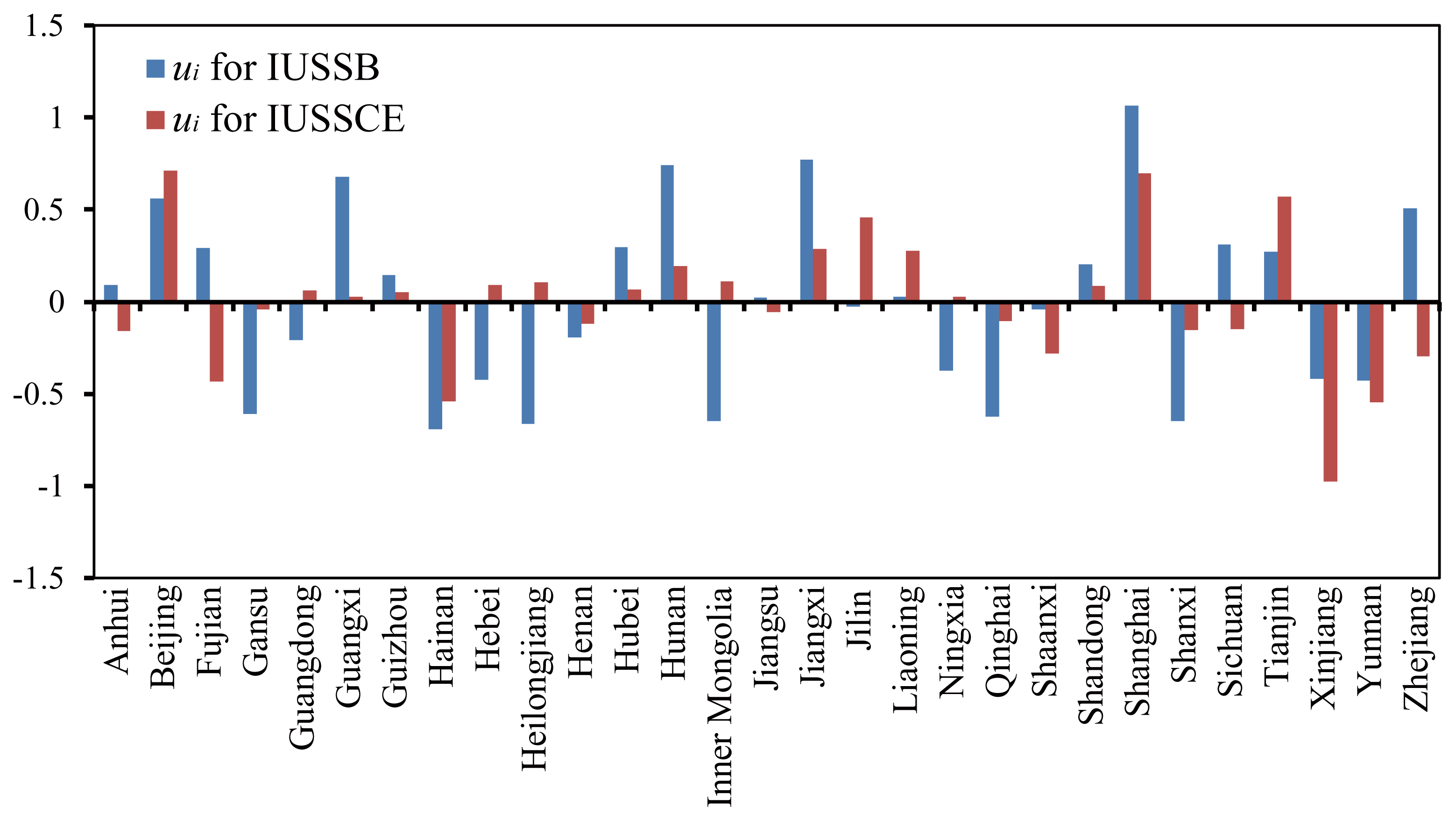
| Anhui | 0.092 | −0.156 |
| Beijing | 0.561 | 0.712 |
| Fujian | 0.289 | −0.433 |
| Gansu | −0.609 | −0.040 |
| Guangdong | −0.210 | 0.063 |
| Guangxi | 0.678 | 0.029 |
| Guizhou | 0.143 | 0.054 |
| Hainan | −0.693 | −0.539 |
| Hebei | −0.421 | 0.091 |
| Heilongjiang | −0.661 | 0.106 |
| Henan | −0.192 | −0.117 |
| Hubei | 0.298 | 0.068 |
| Hunan | 0.744 | 0.197 |
| Inner Mongolia | −0.649 | 0.110 |
| Jiangsu | 0.023 | −0.054 |
| Jiangxi | 0.771 | 0.286 |
| Jilin | −0.027 | 0.459 |
| Liaoning | 0.026 | 0.279 |
| Ningxia | −0.371 | 0.027 |
| Qinghai | −0.623 | −0.105 |
| Shaanxi | −0.041 | −0.281 |
| Shandong | 0.205 | 0.090 |
| Shanghai | 1.067 | 0.698 |
| Shanxi | −0.647 | −0.154 |
| Sichuan | 0.309 | −0.149 |
| Tianjin | 0.270 | 0.573 |
| Xinjiang | −0.415 | −0.973 |
| Yunnan | −0.427 | −0.543 |
| Zhejiang | 0.508 | −0.297 |
Conflicts of Interest
- Author ContributionsHanwei Liang collected and processed the long-term nighttime lights data, performed the regression analysis, results interpretation, manuscript writing, and coordinated the revision activities. Hiroki Tanikawa and Yasunari Matsuno outlined the research topic and assisted with developing the research design, and results interpretation. Liang Dong assisted with refining the research design, interpretation of results and manuscript revision.
References and Notes
- Wong, H.L.; Luo, R.; Zhang, L.; Rozelle, S. Providing quality infrastructure in rural villages: The case of rural roads in China. J. Dev. Econ 2013, 103, 262–274. [Google Scholar]
- Yu, N.; De Jong, M.; Storm, S.; Mi, J. The growth impact of transport infrastructure investment: A regional analysis for China 1978–2008. Policy Soc 2012, 31, 25–38. [Google Scholar]
- Hu, M.; Pauliuk, S.; Wang, T.; Huppes, G.; van der Voet, E.; Müller, D.B. Iron and steel in Chinese residential buildings: A dynamic analysis. Resour. Conserv. Recy 2010, 54, 591–600. [Google Scholar]
- Fernández, J.E. Resource consumption of new urban construction in China. J. Ind. Ecol 2007, 11, 99–115. [Google Scholar]
- Dong, L.; Zhang, H.; Fujita, T.; Ohnishi, S.; Li, H.; Fujii, M.; Dong, H. Environmental and economic gains of industrial symbiosis for Chinese iron/steel industry: Kawasaki’s experience and practice in Liuzhou and Jinan. J. Clean. Prod 2013, 59, 226–238. [Google Scholar]
- World Steel Association, Steel Statistical Yearbook 2013; World Steel Committee on Economic: Brussels, Belgium, 2013.
- Zhu, J.; Lee, K.-K. China steel—Embracing a new age. SCout. 2012. Available online https://research.standardchartered.com/researchdocuments/Pages/ResearchArticle.aspx?&R=98278 (accessed on 19 May 2014).
- Liu, H.; Gallagher, K.S. Catalyzing strategic transformation to a low-carbon economy: A CCS roadmap for China. Energ. Policy 2010, 38, 59–74. [Google Scholar]
- Yang, W.; Kohler, N. Simulation of the evolution of the Chinese building and infrastructure stock. Build. Res. Inf 2008, 36, 1–19. [Google Scholar]
- Hatayama, H.; Daigo, I.; Matsuno, Y.; Adachi, Y. Outlook of the world steel cycle based on the stock and flow dynamics. Environ. Sci. Technol 2010, 44, 6457–6463. [Google Scholar]
- Gordon, R.B.; Bertram, M.; Graedel, T. Metal stocks and sustainability. Proc. Natl. Acad. Sci. USA 2006, 103, 1209–1214. [Google Scholar]
- Müller, D.B.; Wang, T.; Duval, B.; Graedel, T.E. Exploring the engine of anthropogenic iron cycles. Proc. Natl. Acad. Sci. USA 2006, 103, 16111–16116. [Google Scholar]
- Sutton, P.; Roberts, D.; Elvidge, C.; Baugh, K. Census from Heaven: An estimate of the global human population using night-time satellite imagery. Int. J. Remote Sens 2001, 22, 3061–3076. [Google Scholar]
- Doll, C.H.; Muller, J.-P.; Elvidge, C.D. Night-time imagery as a tool for global mapping of socioeconomic parameters and greenhouse gas emissions. AMBIO 2000, 29, 157–162. [Google Scholar]
- Sutton, P.C.; Costanza, R. Global estimates of market and non-market values derived from nighttime satellite imagery, land cover, and ecosystem service valuation. Ecol. Econ 2002, 41, 509–527. [Google Scholar]
- Cao, X.; Wang, J.; Chen, J.; Shi, F. Spatialization of electricity consumption of China using saturation-corrected DMSP-OLS data. Int. J. Appl. Earth Obs 2014, 28, 193–200. [Google Scholar]
- Rauch, J.N. Global mapping of Al, Cu, Fe, and Zn in-use stocks and in-ground resources. Proc. Natl. Acad. Sci. USA 2009, 106, 18920–18925. [Google Scholar]
- Zhang, Q.; Schaaf, C.; Seto, K.C. The Vegetation Adjusted NTL Urban Index: A new approach to reduce saturation and increase variation in nighttime luminosity. Remote Sens. Environ 2013, 129, 32–41. [Google Scholar]
- Hsu, F.C.; Elvidge, C.D.; Matsuno, Y. Exploring and estimating in-use steel stocks in civil engineering and buildings from night-time lights. Int. J. Remote Sens 2013, 34, 490–504. [Google Scholar]
- Matsuno, Y.; Takahashi, K.I.; Adachi, Y.; Nakamura, J.; Elvidge, C. Caluculation of the In-Use Stock of Materials in Urban with Nocturnal Light Image. Proceedings of 2009 Joint Urban Remote Sensing Event, Shanghai, China, 20–22 May 2009; pp. 1–5.
- Hsu, F.C.; Daigo, I.; Matsuno, Y.; Adachi, Y. Estimation of steel stock in building and civil construction by satellite images. ISIJ Int 2011, 51, 313–319. [Google Scholar]
- Hattori, R.; Horie, S.; Hsu, F.-C.; Elvidge, C.D.; Matsuno, Y. Estimation of in-use steel stock for civil engineering and building using nighttime light images. Resour. Conserv. Recy 2013. [Google Scholar] [CrossRef]
- Taguchi, G.; Hsu, F.C.; Tanikawa, H.; Matsuno, Y. Estimation of steel use in buildings by night time light image and GIS. Tetsu-to-Hagane 2012, 98, 450–456. [Google Scholar]
- Hsu, F.C.; Elvidge, C.D.; Matsuno, Y. Estimating in-use steel stock of civil engineering and building in China by nighttime light image. Proc. APAN 2011, 31, 58–68. [Google Scholar]
- Ma, T.; Zhou, C.; Pei, T.; Haynie, S.; Fan, J. Quantitative estimation of urbanization dynamics using time series of DMSP/OLS nighttime light data: A comparative case study from China’s cities. Remote Sens. Environ 2012, 124, 99–107. [Google Scholar]
- Henderson, J.V.; Storeygard, A.; Weil, D.N. Measuring Economic Growth From Outer Space; National Bureau of Economic Research: Cambridge, MA, USA, 2009. [Google Scholar]
- Ghosh, T.; Powell, R.L.; Elvidge, C.D.; Baugh, K.E.; Sutton, P.C.; Anderson, S. Shedding light on the global distribution of economic activity. Open Geogr. J 2010, 3, 148–161. [Google Scholar]
- Kitamura, R. Panel analysis in transportation planning: An overview. Transport. Res. Part A: Gen 1990, 24, 401–415. [Google Scholar]
- Booijink, C.C.G.M.; El-Aidy, S.; Rajilić-Stojanović, M.; Heilig, H.G.H.J.; Troost, F.J.; Smidt, H.; Kleerebezem, M.; De Vos, W.M.; Zoetendal, E.G. High temporal and inter-individual variation detected in the human ileal microbiota. Environ. Microbiol 2010, 12, 3213–3227. [Google Scholar]
- Corbin, A. Country specific effect in the Feldstein–Horioka paradox: A panel data analysis. Econ. Lett 2001, 72, 297–302. [Google Scholar]
- Zhang, C.; Lin, Y. Panel estimation for urbanization, energy consumption and CO2 emissions: A regional analysis in China. Energ. Policy 2012, 49, 488–498. [Google Scholar]
- Han, J.; Xiang, W.-N. Analysis of material stock accumulation in China’s infrastructure and its regional disparity. Sustain. Sci 2013, 8, 553–564. [Google Scholar]
- Zheng, L.; Han, J.; Tanikawa, H. Analysis of material stock accumulated in residential building & transport infrastructures and its regional disparity in China. J. Environ. Inf. Sci 2012, 40, 51–60. [Google Scholar]
- Shi, F.; Huang, T.; Tanikawa, H.; Han, J.; Hashimoto, S.; Moriguchi, Y. Toward a low carbon-dematerialization society measuring the materials demand and CO2 emissions of building and transport infrastructure construction in China. J. Ind. Ecol 2012, 16, 493–505. [Google Scholar]
- Liu, Z.; He, C.; Zhang, Q.; Huang, Q.; Yang, Y. Extracting the dynamics of urban expansion in China using DMSP-OLS nighttime light data from 1992 to 2008. Landscape Urban Plan 2012, 106, 62–72. [Google Scholar]
- Elvidge, C.D.; Ziskin, D.; Baugh, K.E.; Tuttle, B.T.; Ghosh, T.; Pack, D.W.; Erwin, E.H.; Zhizhin, M. A fifteen year record of global natural gas flaring derived from satellite data. Energies 2009, 2, 595–622. [Google Scholar]
- Stewart, J.Q.; Warntz, W. Physics of population distribution. J. Regional Sci 1958, 1, 99–121. [Google Scholar]
- Tobler, W.R. Satellite confirmation of settlement size coefficients. Area 1969, 1, 30–34. [Google Scholar]
- Drukker, D.M. Testing for serial correlation in linear panel-data models. Stata J 2003, 3, 168–177. [Google Scholar]
- Wooldridge, J.M. Econometric Analysis of Cross Section and Panel Data; MIT Press: Cambridge, MA, USA, 2010. [Google Scholar]
- Hausman, J.A. Specification tests in econometrics. Econometrica: J. Econom. Soc 1978, 1251–1271. [Google Scholar]
- Elvidge, C.D.; Baugh, K.E.; Dietz, J.B.; Bland, T.; Sutton, P.C.; Kroehl, H.W. Radiance calibration of DMSP-OLS low-light imaging data of human settlements. Remote Sens. Environ 1999, 68, 77–88. [Google Scholar]
- Mason, L.; Prior, T.; Mudd, G.; Giurco, D. Availability, addiction and alternatives: Three criteria for assessing the impact of peak minerals on society. J. Clean. Prod 2011, 19, 958–966. [Google Scholar]
- Wu, J.; Wang, Z.; Li, W.; Peng, J. Exploring factors affecting the relationship between light consumption and GDP based on DMSP/OLS nighttime satellite imagery. Remote Sens. Environ 2013, 134, 111–119. [Google Scholar]
- Zhang, Q.; Seto, K.C. Can night-time light data identify typologies of urbanization? A global assessment of successes and failures. Remote Sens 2013, 5, 3476–3494. [Google Scholar]
- Tanikawa, H.; Hashimoto, S. Urban stock over time: spatial material stock analysis using 4D-GIS. Build. Res. Inf 2009, 37, 483–502. [Google Scholar]
- Hu, M.; Bergsdal, H.; van der Voet, E.; Huppes, G.; Müller, D.B. Dynamics of urban and rural housing stocks in China. Build. Res. Inf 2010, 38, 301–317. [Google Scholar]
- Doll, C.N.H.; Pachauri, S. Estimating rural populations without access to electricity in developing countries through night-time light satellite imagery. Energ. Policy 2010, 38, 5661–5670. [Google Scholar]
- Small, C.; Elvidge, C.D.; Balk, D.; Montgomery, M. Spatial scaling of stable night lights. Remote Sens. Environ 2011, 115, 269–280. [Google Scholar]
- Gravier-Rymaszewska, J.; Tyrowicz, J.; Kochanowicz, J. Intra-provincial inequalities and economic growth in China. Econ. Systems 2010, 34, 237–258. [Google Scholar] [Green Version]
- Fan, C.C. Interprovincial migration, population redistribution, and regional development in China: 1990 and 2000 census comparisons. Prof. Geogr 2005, 57, 295–311. [Google Scholar]
- Zhao, N.; Ghosh, T.; Samson, E.L. Mapping spatio-temporal changes of Chinese electric power consumption using night-time imagery. Int. J. Remote Sens 2012, 33, 6304–6320. [Google Scholar]
- Zhang, Q.; Seto, K.C. Mapping urbanization dynamics at regional and global scales using multi-temporal DMSP/OLS nighttime light data. Remote Sens. Environ 2011, 115, 2320–2329. [Google Scholar]
- Démurger, S. Infrastructure development and economic growth: An explanation for regional disparities in China? J. Comp. Econ 2001, 29, 95–117. [Google Scholar]
- Letu, H.; Hara, M.; Tana, G.; Nishio, F. A. Saturated light correctionmethod for DMSP/OLS nighttime satellite imagery. IEEE Trans. Geosci. Remote Sens 2012, 50, 389–396. [Google Scholar]
- Shi, K.; Yu, B.; Huang, Y.; Hu, Y.; Yin, B.; Chen, Z.; Chen, L.; Wu, J. Evaluating the ability of NPP-VIIRS nighttime light data to estimate the gross domestic product and the electric power consumption of China at multiple scales: A comparison with DMSP-OLS data. Remote Sens 2014, 6, 1705–1724. [Google Scholar]
- Eisner, R. Infrastructure and regional economic performance: Comment. New Engl. Rev 1991, 74, 47–58. [Google Scholar]
- Holtz-Eakin, D.; Schwartz, A.E. Infrastructure in a structural model of economic growth. Reg. Sci. Urban Econ 1995, 25, 131–151. [Google Scholar]
- Czernich, N.; Falck, O.; Kretschmer, T.; Woessmann, L. Broadband infrastructure and economic growth*. Econ. J 2011, 121, 505–532. [Google Scholar]
- Sahoo, P.; Dash, R.K. Economic growth in South Asia: Role of infrastructure. J. Int. Trade Econ. Dev 2012, 21, 217–252. [Google Scholar]
- Milford, R.L.; Pauliuk, S.; Allwood, J.M.; Müller, D.B. The roles of energy and material efficiency in meeting steel industry CO2 targets. Environ. Sci. Technol 2013, 47, 3455–3462. [Google Scholar]
- Pauliuk, S.; Wang, T.; Müller, D.B. Steel all over the world: Estimating in-use stocks of iron for 200 countries. Resour. Conserv. Recy 2013, 71, 22–30. [Google Scholar] [Green Version]
- Pauliuk, S.; Wang, T.; Muller, D.B. Moving toward the circular economy: The role of stocks in the Chinese steel cycle. Environ. Sci. Technol 2012, 46, 148–154. [Google Scholar]


| Satellite | Year | IUSSB | IUSSCE | R2avg | ||||||
|---|---|---|---|---|---|---|---|---|---|---|
| βbuilding | kbuilding | R2building | RMSE | βcivil | kcivil | R2civil | RMSE | |||
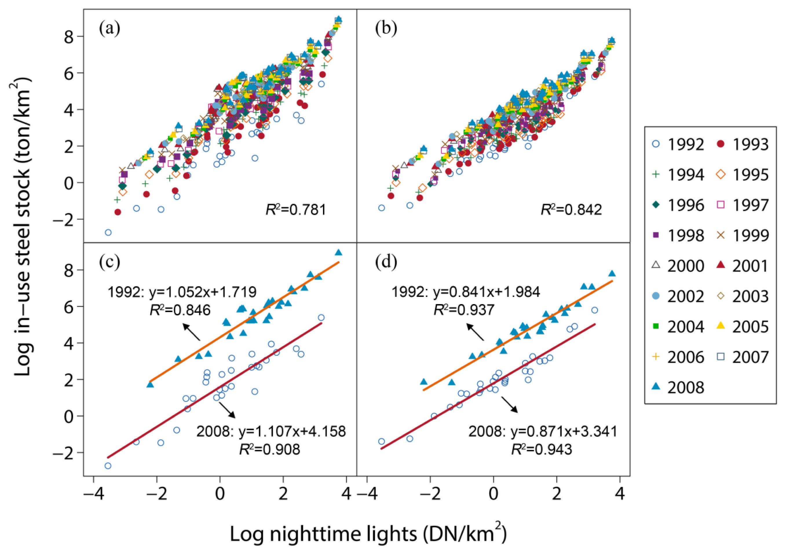
| F10 | 1992 | 1.052 | 1.719 | 0.846 | 0.713 | 0.841 | 1.984 | 0.937 | 0.347 | 0.892 |
| F10 | 1993 | 1.024 | 2.265 | 0.884 | 0.575 | 0.801 | 2.146 | 0.927 | 0.349 | 0.906 |
| F10 | 1994 | 1.003 | 2.687 | 0.891 | 0.541 | 0.768 | 2.331 | 0.916 | 0.359 | 0.904 |
| F12 | 1994 | 0.988 | 2.728 | 0.893 | 0.538 | 0.749 | 2.365 | 0.901 | 0.389 | 0.897 |
| F12 | 1995 | 0.988 | 2.950 | 0.891 | 0.536 | 0.745 | 2.469 | 0.911 | 0.360 | 0.901 |
| F12 | 1996 | 0.997 | 3.166 | 0.888 | 0.541 | 0.741 | 2.610 | 0.907 | 0.362 | 0.898 |
| F12 | 1997 | 1.003 | 3.317 | 0.885 | 0.547 | 0.742 | 2.721 | 0.906 | 0.362 | 0.896 |
| F12 | 1998 | 1.038 | 3.502 | 0.898 | 0.525 | 0.77 | 2.817 | 0.910 | 0.355 | 0.904 |
| F12 | 1999 | 1.020 | 3.825 | 0.908 | 0.512 | 0.746 | 3.042 | 0.898 | 0.365 | 0.903 |
| F14 | 1997 | 1.009 | 3.362 | 0.884 | 0.549 | 0.739 | 2.758 | 0.888 | 0.396 | 0.886 |
| F14 | 1998 | 1.010 | 3.480 | 0.903 | 0.518 | 0.75 | 2.800 | 0.908 | 0.352 | 0.906 |
| F14 | 1999 | 1.014 | 3.658 | 0.904 | 0.520 | 0.755 | 2.911 | 0.909 | 0.358 | 0.907 |
| F14 | 2000 | 1.051 | 3.758 | 0.879 | 0.595 | 0.788 | 2.969 | 0.909 | 0.356 | 0.894 |
| F14 | 2001 | 1.041 | 3.949 | 0.890 | 0.537 | 0.802 | 3.107 | 0.931 | 0.323 | 0.911 |
| F14 | 2002 | 1.058 | 4.009 | 0.915 | 0.451 | 0.801 | 3.172 | 0.923 | 0.324 | 0.919 |
| F14 | 2003 | 1.064 | 4.040 | 0.924 | 0.425 | 0.817 | 3.201 | 0.927 | 0.319 | 0.926 |
| F15 | 2000 | 1.018 | 3.783 | 0.886 | 0.530 | 0.764 | 2.988 | 0.916 | 0.336 | 0.901 |
| F15 | 2001 | 1.016 | 3.914 | 0.895 | 0.523 | 0.78 | 3.082 | 0.927 | 0.306 | 0.911 |
| F15 | 2002 | 1.031 | 3.982 | 0.913 | 0.446 | 0.791 | 3.143 | 0.930 | 0.302 | 0.922 |
| F15 | 2003 | 1.046 | 4.019 | 0.925 | 0.421 | 0.813 | 3.176 | 0.931 | 0.307 | 0.928 |
| F15 | 2004 | 1.061 | 4.064 | 0.907 | 0.513 | 0.825 | 3.206 | 0.939 | 0.291 | 0.923 |
| F15 | 2005 | 1.091 | 4.167 | 0.905 | 0.517 | 0.856 | 3.297 | 0.952 | 0.274 | 0.929 |
| F15 | 2006 | 1.101 | 4.181 | 0.915 | 0.458 | 0.866 | 3.331 | 0.943 | 0.286 | 0.929 |
| F15 | 2007 | 1.117 | 4.182 | 0.928 | 0.453 | 0.871 | 3.358 | 0.952 | 0.278 | 0.940 |
| F16 | 2004 | 1.098 | 3.963 | 0.911 | 0.476 | 0.854 | 3.128 | 0.943 | 0.283 | 0.927 |
| F16 | 2005 | 1.071 | 4.111 | 0.911 | 0.477 | 0.835 | 3.259 | 0.951 | 0.259 | 0.931 |
| F16 | 2006 | 1.078 | 4.147 | 0.917 | 0.442 | 0.849 | 3.303 | 0.945 | 0.279 | 0.931 |
| F16 | 2007 | 1.095 | 4.157 | 0.932 | 0.413 | 0.857 | 3.335 | 0.950 | 0.269 | 0.941 |
| F16 | 2008 | 1.107 | 4.158 | 0.908 | 0.462 | 0.871 | 3.341 | 0.943 | 0.280 | 0.926 |
| Province | IUSSB | IUSSCE | R2avg | ||||||
|---|---|---|---|---|---|---|---|---|---|
| βbuilding | kbuilding | R2building | RMSE | βcivil | kcivil | R2civil | RMSE | ||
| Anhui | 2.345 | 2.720 | 0.972 | 0.165 | 1.784 | 1.790 | 0.989 | 0.079 | 0.981 |
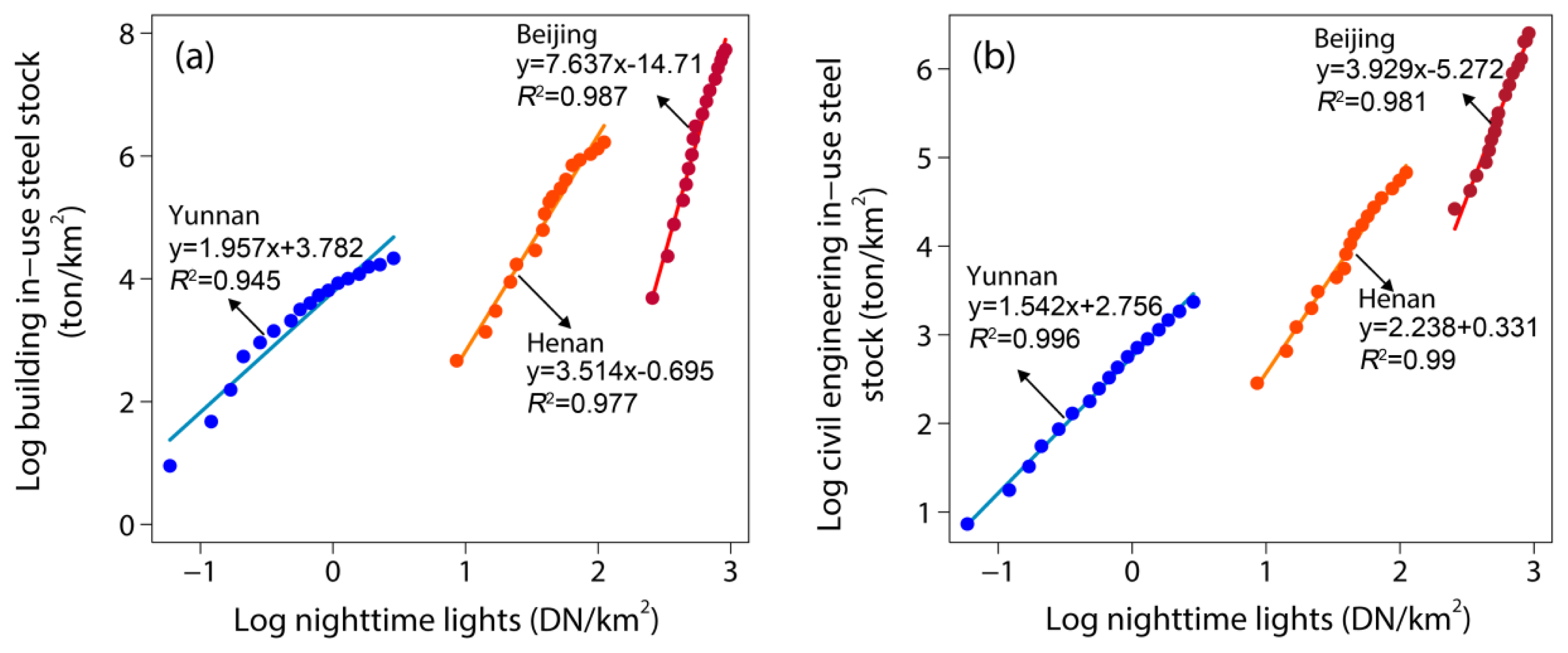
| Beijing | 7.637 | −14.71 | 0.987 | 0.143 | 3.929 | −5.272 | 0.981 | 0.088 | 0.984 |
| Fujian | 2.872 | 1.961 | 0.966 | 0.192 | 2.091 | 1.108 | 0.976 | 0.115 | 0.971 |
| Gansu | 3.035 | 4.662 | 0.914 | 0.349 | 1.913 | 3.954 | 0.947 | 0.169 | 0.931 |
| Guangdong | 4.061 | −2.574 | 0.956 | 0.201 | 3.467 | −2.456 | 0.958 | 0.169 | 0.957 |
| Guangxi | 2.737 | 4.033 | 0.964 | 0.219 | 1.945 | 2.769 | 0.981 | 0.111 | 0.973 |
| Guizhou | 2.646 | 4.349 | 0.979 | 0.190 | 1.502 | 3.380 | 0.972 | 0.125 | 0.976 |
| Hainan | 1.917 | 2.382 | 0.978 | 0.128 | 1.499 | 1.875 | 0.951 | 0.150 | 0.965 |
| Hebei | 4.323 | −2.519 | 0.955 | 0.206 | 3.409 | −1.771 | 0.963 | 0.148 | 0.959 |
| Heilongjiang | 3.184 | 2.380 | 0.928 | 0.291 | 2.128 | 2.597 | 0.924 | 0.199 | 0.926 |
| Henan | 3.514 | −0.695 | 0.977 | 0.172 | 2.238 | 0.331 | 0.990 | 0.071 | 0.984 |
| Hubei | 3.662 | 1.925 | 0.950 | 0.280 | 1.966 | 2.320 | 0.990 | 0.066 | 0.970 |
| Hunan | 2.625 | 4.198 | 0.931 | 0.318 | 1.606 | 3.090 | 0.970 | 0.125 | 0.951 |
| Inner Mongolia | 3.181 | 5.592 | 0.903 | 0.427 | 1.900 | 4.510 | 0.900 | 0.259 | 0.902 |
| Jiangsu | 3.489 | −2.248 | 0.952 | 0.241 | 2.706 | −1.813 | 0.965 | 0.159 | 0.959 |
| Jiangxi | 2.191 | 4.528 | 0.873 | 0.396 | 1.687 | 3.124 | 0.925 | 0.228 | 0.899 |
| Jilin | 3.369 | 2.146 | 0.892 | 0.338 | 2.620 | 2.108 | 0.946 | 0.180 | 0.919 |
| Liaoning | 5.083 | −2.695 | 0.969 | 0.183 | 2.973 | −0.141 | 0.971 | 0.104 | 0.970 |
| Ningxia | 3.034 | 2.116 | 0.969 | 0.187 | 2.407 | 2.028 | 0.960 | 0.168 | 0.965 |
| Qinghai | 2.494 | 7.396 | 0.871 | 0.463 | 1.611 | 5.464 | 0.934 | 0.206 | 0.903 |
| Shaanxi | 3.133 | 2.063 | 0.888 | 0.413 | 2.046 | 1.814 | 0.976 | 0.118 | 0.932 |
| Shandong | 3.142 | −0.701 | 0.932 | 0.225 | 2.935 | −1.842 | 0.967 | 0.143 | 0.950 |
| Shanghai | 5.705 | −12.520 | 0.953 | 0.234 | 3.179 | −5.081 | 0.957 | 0.125 | 0.955 |
| Shanxi | 5.015 | −3.662 | 0.988 | 0.124 | 3.412 | −1.624 | 0.979 | 0.112 | 0.984 |
| Sichuan | 2.756 | 4.390 | 0.955 | 0.306 | 1.422 | 3.264 | 0.992 | 0.064 | 0.974 |
| Tianjin | 6.806 | −13.840 | 0.975 | 0.192 | 3.262 | −3.968 | 0.973 | 0.095 | 0.974 |
| Xinjiang | 2.836 | 6.744 | 0.970 | 0.234 | 1.743 | 4.054 | 0.984 | 0.103 | 0.977 |
| Yunnan | 1.957 | 3.782 | 0.945 | 0.232 | 1.542 | 2.756 | 0.996 | 0.047 | 0.971 |
| Zhejiang | 2.476 | 1.464 | 0.942 | 0.256 | 1.867 | 0.698 | 0.968 | 0.141 | 0.955 |
| β | k | N (obs.) | N (group) | R2 (adjusted) | RMSE | ρ(ar) | σ(e) | σ(u) | ρ(fov) | |
|---|---|---|---|---|---|---|---|---|---|---|
| IUSSB | 0.868 *** | 1.737 *** | 464 | 29 | 0.900 | 0.558 | 0.856 | 0.098 | 0.473 | 0.959 |
| IUSSCE | 0.656 *** | 2.001 *** | 464 | 29 | 0.914 | 0.374 | 0.880 | 0.053 | 0.279 | 0.959 |
| Models | IUSSB | IUSSCE | ||||||||
| c0 | c1 | c2 | R2 | RMSE | c0 | c1 | c2 | R2 | RMSE | |
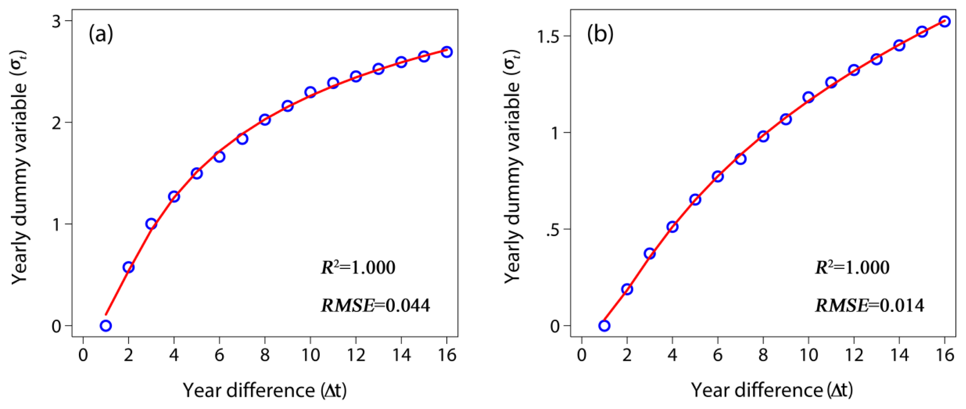
| 0.767 *** | −2.976 *** | 0.150 ** | 1.000 | 0.044 | −0.506 *** | −2.949 *** | 0.414 *** | 1.000 | 0.014 | |
© 2014 by the authors; licensee MDPI, Basel, Switzerland This article is an open access article distributed under the terms and conditions of the Creative Commons Attribution license (http://creativecommons.org/licenses/by/3.0/).
Share and Cite
Liang, H.; Tanikawa, H.; Matsuno, Y.; Dong, L. Modeling In-Use Steel Stock in China’s Buildings and Civil Engineering Infrastructure Using Time-Series of DMSP/OLS Nighttime Lights. Remote Sens. 2014, 6, 4780-4800. https://doi.org/10.3390/rs6064780
Liang H, Tanikawa H, Matsuno Y, Dong L. Modeling In-Use Steel Stock in China’s Buildings and Civil Engineering Infrastructure Using Time-Series of DMSP/OLS Nighttime Lights. Remote Sensing. 2014; 6(6):4780-4800. https://doi.org/10.3390/rs6064780
Chicago/Turabian StyleLiang, Hanwei, Hiroki Tanikawa, Yasunari Matsuno, and Liang Dong. 2014. "Modeling In-Use Steel Stock in China’s Buildings and Civil Engineering Infrastructure Using Time-Series of DMSP/OLS Nighttime Lights" Remote Sensing 6, no. 6: 4780-4800. https://doi.org/10.3390/rs6064780