Estimating Canopy Nitrogen Content in a Heterogeneous Grassland with Varying Fire and Grazing Treatments: Konza Prairie, Kansas, USA

Abstract

Quantitative, spatially explicit estimates of canopy nitrogen are essential for understanding the structure and function of natural and managed ecosystems. Methods for extracting nitrogen estimates via hyperspectral remote sensing have been an active area of research. Much of this research has been conducted either in the laboratory, or in relatively uniform canopies such as crops. Efforts to assess the feasibility of the use of hyperspectral analysis in heterogeneous canopies with diverse plant species and canopy structures have been less extensive. In this study, we use in situ and aircraft hyperspectral data to assess several empirical methods for extracting canopy nitrogen from a tallgrass prairie with varying fire and grazing treatments. The remote sensing data were collected four times between May and September in 2011, and were then coupled with the field-measured leaf nitrogen levels for empirical modeling of canopy nitrogen content based on first derivatives, continuum-removed reflectance and ratio-based indices in the 562–600 nm range. Results indicated that the best-performing model type varied between in situ and aircraft data in different months. However, models from the pooled samples over the growing season with acceptable accuracy suggested that these methods are robust with respect to canopy heterogeneity across spatial and temporal scales.

1. Introduction

Research efforts into grassland ecosystems are substantial [1–4], given that grasslands are the potential vegetation covering approximately 36% of the earth’s surface [5], and one of the largest vegetative provinces in North America [6]. Along with fire and climate, herbivore grazing plays a central role in altering the structure and function of grassland ecosystems [7–9]. Grassland heterogeneity is a major outcome of fire and grazing activities, which in turn affects future forage pattern of grazers. This interplay between grassland heterogeneity and grazing pattern is of great interest [10,11] due to its significant influences on grassland processes through nutrient redistribution and cycling. Quantitative estimates of canopy biochemical properties are essential for understanding the forage quality distribution and heterogeneity in grassland ecosystems. Among the more important of these biochemical properties is foliar nitrogen content. Nitrogen (N) is an indispensable element in the composition of amino and nucleic acids in all living organisms and an often limiting nutrient in natural ecosystems including grasslands [12]. N cycling is a key biogeochemical flux through the earth system, where vegetation is involved in uptake, storage and exchange with other components of the system. Understanding the concentration and distribution of N within vegetative canopies is therefore important for addressing a wide variety of applied and systemic questions in biospheric science.

There is widespread interest in developing methods to estimate the distribution of foliar quality of vegetation canopies using remote sensing [13,14]. Traditional methods for measuring nitrogen in vegetative canopies based on laboratory chemical analysis of field-collected foliar samples are complex and expensive. This is especially true when a large number of samples are needed to adequately characterize N distribution over a relatively large area. To address such questions using traditional methods, samples typically consisting of a few grams of canopy material must be collected from point sites distributed throughout the area of interest. Each individual sample represents only a few square centimeters of the canopy, thus some sort of spatial interpolation/extrapolation scheme must be used to estimate values between the point samples if nitrogen is to be mapped over an extensive area. Interpolation schemes can themselves be a significant source of error.

In general, remote sensing based methods for retrieving canopy nitrogen have used high spectral resolution (hyperspectral) reflectance spectra collected from leaf or canopy surfaces [13,15–18]. Remote sensing of canopy nitrogen is complicated by the interaction of light in the VNIR/SWIR (400–2500 nm) spectral region with nitrogen in foliar tissues. Nitrogen in foliar tissues directly affects the reflectance spectrum resulting from absorption features due to molecular nitrogen in these reflectance spectra [19]. However, the relevant spectral regions for direct analysis of canopy N are in the SWIR spectral region, and are thus not accessible to spectrometers or imaging system which lack sensitivity in this region. Other commonly used methods for retrieving estimates of N from vegetation canopies depend on indirect estimates that exploit the fact that foliar nitrogen is concentrated in plant chloroplasts [20,21]. Chlorophyll absorption bands are very prominent in the visible region of the spectrum, and are readily accessible to current remote sensing detectors. The efficacy of using the indirect methods in remote sensing studies for estimating nitrogen concentration via the use of chlorophyll absorption features is now well known and widely used [22–26].

A main challenge of retrieving canopy-level N using remote sensing is that the structure and composition of vegetation canopies is complex, affecting the reflectance of the canopy and therefore the signal received by the sensor. Even relatively homogeneous canopies such as crops are structurally complex mixtures of living and senescent plant tissues, stems and other components. These diverse materials, which in sparse canopies may also include the soil background, are integrated within the field of view of the remote sensor, producing a mixture of spectral elements in the received signal. In heterogeneous canopies (e.g., grasslands) with a diverse mixture of species and growth forms, the signal received at-sensor can be an even more complex mixture spectral responses from diverse reflective materials [13,27].

Available methods for normalizing spectral signals to minimize the effects of canopy heterogeneity have mainly concentrated on removing background effects in order to “isolate” the biochemical signal of interest. These methods include: (1) use of the first derivative of the spectral reflectance curve and (2) continuum removal [28–30]. The first derivative of reflectance characterizes the changes of the original reflectance by which the background effects are countervailed [31]. Continuum removal provides a common baseline that allows the spectral features to be standardized and compared [21,32]. Additionally, hyperspectral vegetation indices (VIs) integrating spectral values at different wavelengths can normalize spectral features [33–35] and are thus potentially applicable to the canopy heterogeneity problem. The standardized difference between two spectral values is the most commonly used form of VI, due to its inherent scaling of the spectral signals and reduced sensitivity to background variations [27,36].

The results we present here are part of a larger project aimed at understanding the relationship between canopy nutrient quality and grazer behavior in tallgrass prairie. The interaction between distribution of foliar nutrients (e.g., N) in a grassland canopy and the forage pattern of ungulate grazers is of special interest since these grazing activities alter the structure and composition of vegetation and therefore influence vegetation quality [37,38]. Grazed sites often yield higher nutritional value with greater plant species diversity than do ungrazed sites [39–41] due to the capability of plants to overcompensate with regrowth for low levels of herbivory [42]. Vegetation quality is one of the major factors that influence grazing strategies of herbivores, and the sites with higher nutrient concentration are likely to be more frequently used by grazers [1,3]. Canopy N is a key index of grassland forage quality, and detailed information on its spatial and temporal distribution derived from remote sensing is essential to the goals of this research.

The problem of remote sensing nitrogen in tallgrass prairie canopies is conceptually similar to other canopies, although in practice it is complicated by the heterogeneity problem discussed above. Among grassland canopies, tallgrass prairie is especially heterogeneous, consisting of a diverse, intermingled mix of herbaceous and woody species. Several interacting biophysical factors, including fire, topography, and grazing determine this complex spatial distribution of canopy properties [38,43]. Tallgrass prairie canopies can have more than twenty species present in a single square meter, each with different growth forms and leaf structure, thus producing a closely intermingled mixture of species. In addition, these intermingled species often have different photosynthetic pathways. Most of the graminoids (grasses and sedges) are C4 plants, they photosynthesize via a pathway in which the first intermediate product is a 4-carbon molecule. The majority of forbs (flowering species) are C3 photosynthesizers, whose first intermediate product is a 3-carbon molecule. In general, C4 plants tolerate temperature extremes better than C3s [44]. All these factors influence the spectral response of the canopy, making the aggregate reflectance signal from even a small area of the canopy a complicated mixture of individual components, and potentially making the retrieval of biophysical information from tallgrass prairie much more difficult. Our objective is to develop and evaluate empirical models using hyperspectral remote sensing data that can be used for estimating and mapping canopy nitrogen in tallgrass prairie canopies.

2. Study Site

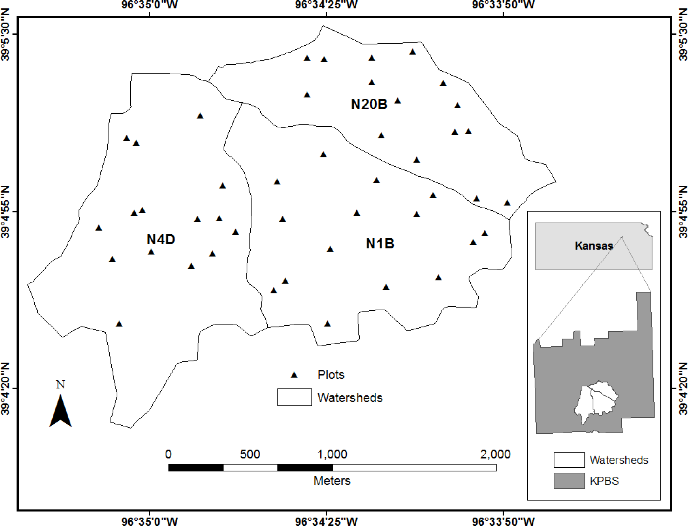
This research was conducted at the Konza Prairie Biological Station (KPBS), near Manhattan, KS, USA (39°05′N, 96°35′W, Figure 1). KPBS is located in the Flint Hills, the largest extant area of tallgrass prairie in North America. The site covers an area of 34.87 km², and is characterized by a continental climate with warm, wet springs, hot summers and dry, cold winters. Approximately 75% of the annual precipitation (∼826 mm) is concentrated during the period from April to September, supporting vegetation growth in the prairie. The vegetation in KPBS is characterized by C4 perennial grasses interspersed with C3 forbs and a few C3 grasses, resulting in great species diversity. Grasses compose 80%–90% of total vegetation cover; dominant grass species include Andropogon gerardii, Sorghastrum nutans, Bouteloua gracilis, Panicum virgatum, and Schizachyrium scoparium. Forbs constitute a minor component of the canopy but account for much of the species diversity. Common forbs include Aster ericoides, Psoralea tenuiflora, Solidago missouriensis, Soldiago rigida, Liaris aspera, Vernonia baldwinii and Ambrosia psilostachya [38,45].

A long term watershed-level experiment at KPBS is designed to investigate the effects of fire and grazing on the structure and function of the tallgrass prairie vegetative community. The site is divided into more than 50 watersheds, each with varying combinations of fire return frequencies (1,2,4,10, and 20 years) and one of three grazing treatments (grazed by American bison (Bison bison), grazed by domesticated cattle (Bos taurus), and ungrazed). Since this research was conducted as part of a larger study of grazing behavior in Bison bison, we selected three watersheds (with a total area of ∼3.40 km²) in the bison grazing area for our analysis (see Figure 1 for locations of selected watersheds). In situ hyperspectral data and foliar samples were collected in three watersheds (N1B, N4D and N20B) with fire frequencies of one year, four years and 20 years, respectively. Variations in fire frequency influence the proportion of green vegetation, senescent materials, stems, and litter in the canopy, which in turn influences spatial patterns of grazing by bison [46–48]. All of these fire-related factors contribute to a complex, spatially variable canopy. Thus, our selected combination of fire and grazing treatments yields a study area with widely varying species composition and canopy density, resulting in a very heterogeneous canopy.

3. Data and Methods

3.1. Data Collection

Data were collected on four dates spanning the 2011 growing season. Each data collection effort consisted of a field component (

Table 1. Datasets of in situ measurements.

Dates	# of Samples	Data Collected
12–13 May	45	Spectral, N samples
29 June–1 July	45	Spectral, N samples, Ceptometry
1–2 August	45	Spectral, N samples, Ceptometry
11 September	27	Spectral, N samples

), coordinated with an aircraft overflight. Field data were collected from fifteen 10 m × 10 m plots randomly distributed in each of the three designated watersheds, giving a total of 45 sampling sites. Random selection of sites ensured that the samples we collected were representative of species composition over the entire watershed. Technical problems limited the usable data from the September field survey to only 27 sites.

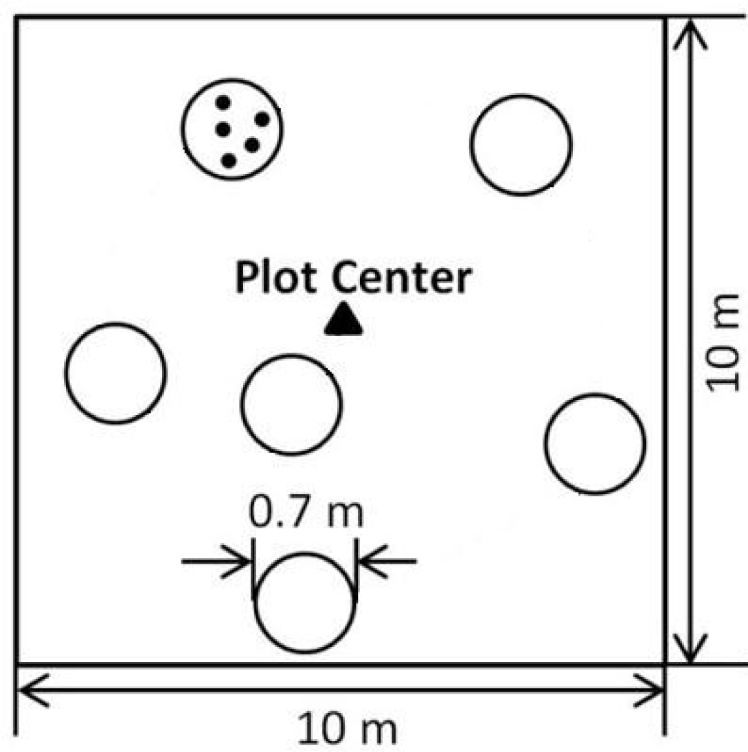
In each plot, subsamples consisting of six randomly selected points were distributed around the center of the plot (Figure 2). Two types of nondestructive data sampling were performed at each site, (1) spectral reflectance; and (2) PAR (above and below canopy). In addition, a destructive sample of plant tissue was collected for laboratory analysis of nitrogen content. Hyperspectral reflectance data were taken for each subplot using an Analytical Spectral Devices (ASD) FieldSpec Pro portable spectrometer (Analytical Spectral Devices, Boulder, CO, USA). Spectra were collected from a height of 1.5 m above the target using a 25° field of view optic, yielding a ∼0.4 m² circular field of view, with a diameter of ∼0.7 m on the target. The acquired reflected spectra range from 350 to 2500 nm, with spectral resolution ranging from ∼3 nm at the 700 nm wavelength to 10–12 nm for wavelengths of 1050–2500 nm. Individual spectra were converted to reflectance by normalization to a Spectralon reflectance standard. For each plot, a single spectrum was calculated by averaging the reflectance values of each wavelength from the spectra collected from each subplot. On two of the four sampling dates (29 June–1 July and 1–2 August 2011), PAR samples were collected from the same IFOV as the spectral data using an Accupar LP-80 line ceptometer. Geographic coordinates for the center of each plot were collected using a portable GPS receiver.

Immediately following the non-destructive sampling, five foliar samples from each of the six subplots, representative of the plant species (grasses and forbs) in each subplot, were clipped from the same IFOV as the spectral and PAR data. In the laboratory, these samples were mixed and ground after drying at 60 °C for 48 h. Dried ground samples from three randomly selected subplots of the six, sufficient to characterize the N status in the whole plot, were then used for foliar nitrogen concentration determination by laboratory elemental analysis using a Costech ECS 4010 (Costech Analytical Technologies Inc., Valencia, CA, USA). Foliar nitrogen content for each plot was determined by averaging the values from the three samples.

Hyperspectral imagery were collected concurrently with each field sampling session using an AISA Eagle camera mounted on a Piper Warrior aircraft operated by the Center for Advanced Land Management Information Technology (CALMIT) of the University of Nebraska-Lincoln. On each date, 4–5 lines were flown, covering the whole area of KPBS and including the three watersheds used in this analysis. The aircraft was flown at an altitude yielding a spatial resolution of 2 m × 2 m. Spectral resolution varied between ∼3 nm for the May–August flights, and ∼10 nm for the September flight. The camera was configured with a spectral range from 435 to 950 nm (note that the ASIA Eagle is not sensitive beyond 970 nm).

3.2. Data Analysis

3.2.1. Canopy Nitrogen Calculation

Since our interest was in estimating canopy nitrogen content, converting leaf nitrogen (N_leaf) samples to canopy scale was a key step in data analysis. Nitrogen content can be scaled from the leaf to the canopy level using the canopy-integrated method [49], which relates canopy nitrogen (N_can) to N_leaf with respect to a leaf area index (LAI):

$$N_{\mathit{can}}=N_{\mathit{leaf}}\times \mathit{LAI}$$

(1)

LAI can be estimated from above and below canopy PAR measurements using:

$$\mathit{LAI}=-2\text{cos}\theta \times \text{ln}\frac{\mathit{PA}{\mathit{R}}_{\mathit{below}}}{\mathit{PA}{\mathit{R}}_{\mathit{above}}}$$

(2)

where θ is the solar zenith angle. As earlier noted, direct ceptometric PAR measurements were not available for all of the data collection periods. In addition, PAR-method was limited in senescent canopies, which usually overestimated the green LAI. We therefore used an alternative method of calculating LAI, based on the Normalized Difference Vegetation Index (NDVI):

$$\mathit{LAI}=0.08\times e^{3.706\times \mathit{NDVI}}$$

(3)

where NDVI was calculated from the ASD reflectance values by integrating the wavelengths of 780–800 nm for broadband red reflectance, and 670–678 nm for the broadband NIR. This empirical relationship was validated using data of the two dates for which both ceptometry and spectral reflectance were available, and was found to be reasonably accurate (R* = 0.85, based on jackknife analysis with sample size = 27) [50].

3.2.2. Spectral Reflectance Indices Calculation—Field-Collected Spectra

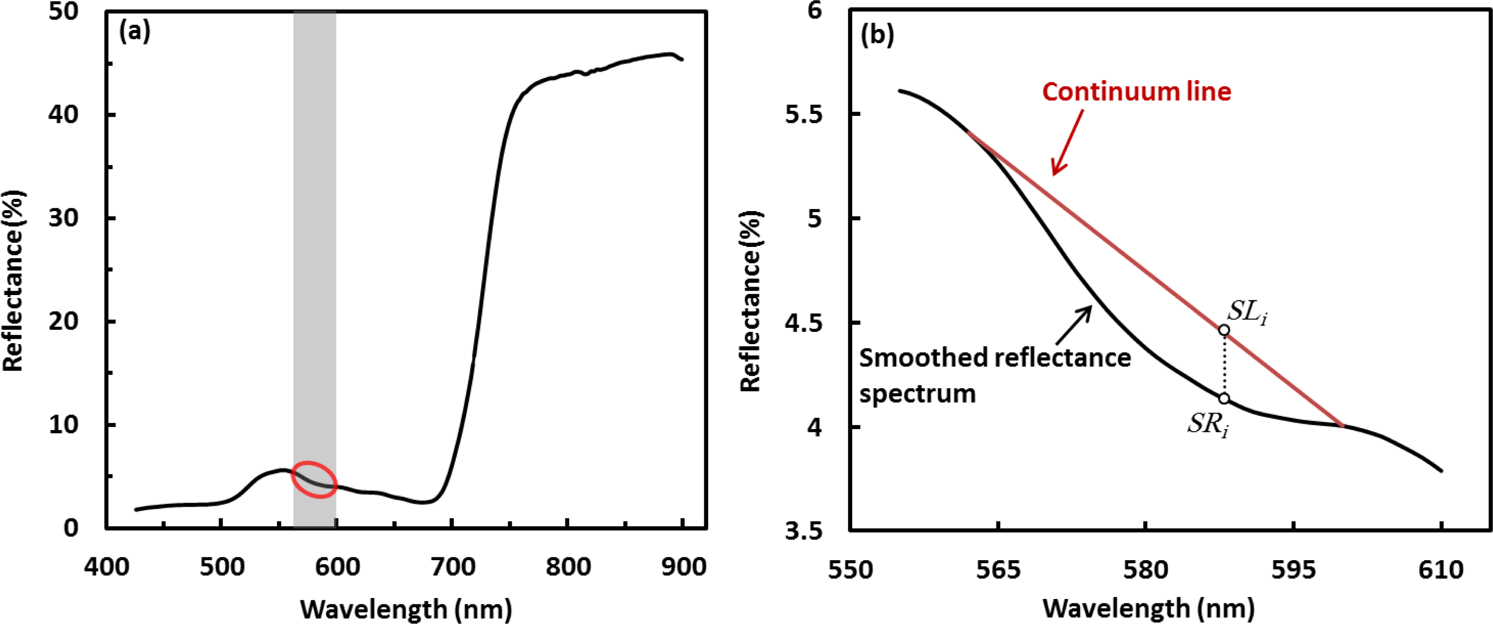
Preparation of the field measured spectral reflectance data for analysis consisted of numerical differentiation of the spectral curves, continuum removal, and calculation of relevant vegetation indices. Both the first derivative calculation and continuum removal are sensitive to random noise in the spectral signal, so the raw reflectance spectra were smoothed prior to further analysis using a three-point moving average filter. Because the actual spectral resolution of the spectrometer is ∼3 nm, we resampled the field spectra by averaging reflectance at every three nanometer increments into one value, similar to the way in which the aircraft sensor sampled spectra. The first derivative of reflectance, a transformation which has been shown to be useful for extracting biophysical information from spectral curves [28,31], was calculated in the spectral region of 562–600 nm. This spectral region has a subtle absorption feature (Figure 3a) sensitive to leaf chlorophyll concentration [51,52], and leaf chlorophyll concentration has been demonstrated to be linked with foliar nitrogen more or less [20,21,53,54]. As earlier noted, we did not use the nitrogen absorption feature centered at 1510 nm because the spectral range of the aircraft-mounted sensor (435–950 nm) does not include the SWIR spectral region. The ASD spectrometer does include this region, but we elected not to use it in order to keep the methods applied to both the field and aircraft data sets as parallel as possible. Derivatives were calculated using:

$$D_i=\frac{\mathit{S}{\mathit{R}}_{i+1}-\mathit{S}{\mathit{R}}_{i-1}}{{\lambda }_{i+1}-{\lambda }_{i-1}}$$

(4)

where D_i is the first derivative at the wavelength i; SR_i is the smoothed reflectance value at the wavelength i, and λ_i is the value of the wavelength i.

Continuum removal standardizes the canopy spectral signals using a linear hull (continuum line) to fit over the top of a given absorption feature in the spectrum [29,30]. The continuum removed spectral value at a wavelength is calculated as the ratio of the value in the reflectance spectrum to the corresponding value in the continuum removal line at the given wavelength (Figure 3b). We used the same absorption feature for continuum removal (562–600 nm) that we used for the first derivative calculation, for the same reasons. The continuum removed value at each wavelength was calculated as:

$$\mathit{C}{\mathit{R}}_i=\frac{\mathit{S}{\mathit{R}}_i}{\mathit{S}{\mathit{L}}_i}$$

(5)

where CR_i is the continuum removed spectral value at the wavelength i; SR_i is the smoothed reflectance at the wavelength i; and SL_i is the value at the wavelength i in the continuum line fitted over the absorption spectral feature.

The standardized difference vegetation index (SDVI) was developed for various derivative and continuum removed spectral features using:

$$\mathit{SDV}{\mathit{I}}_i=\frac{{\mathit{S}}_i-S_j}{{\mathit{S}}_i+S_j}$$

(6)

where Si is the spectral feature at the wavelength i. SDVI derives from the theoretical underpinning of ratio-based vegetation indices such as NDVI [55] that scales the difference in two spectral features which behavior diversely.

3.2.3. Spectral Reflectance and Indices Calculation—Aircraft-Collected Spectra

Aerial imagery was processed using the ENvironment for Visualizing Images (ENVI) software (Exelis Visual Information Solutions, Inc., Boulder, CO, USA). Prior to analysis, the FLAASH model implemented within ENVI was used for atmospheric correction. For each of the four FLAASH runs, the atmospheric model was set to midlatitude summer and the aerosol model to rural. Visibility for each day was estimated using meteorological optical range (MOR) data from the Topeka, KS, National Weather Service station (located approximately 80 km from the study site). Visibilities were 16 km for the May, July and August acquisitions, and 14 km for the September acquisition. Since our analysis was restricted only to grassland canopies, supervised Maximum Likelihood classification was used to classify land cover on the four images captured during May–September into four classes, including gallery forests (i.e., wooded areas along drainages), roads, sparse grasses and dense grasses. The gallery forest areas and the roads were masked from the imagery and not included in subsequent analysis. Since the gallery forests were expanding during the growing seasons, the forest mask varied over time. A union of masks for the four data collection sessions was built and applied to make sure that the mask looked the same and all forested pixels were removed.

Plots for in situ data collection were located on aerial imagery using the plot center coordinates collected in the field. Spectral data from airborne imagery for each plot were obtained by calculating the mean of spectral reflectance data within a window of 5 pixel × 5 pixel (10 m × 10 m) centered around the plot center on the imagery. These averaged values were then subjected to the same analysis (smoothing, continuum removal, numerical differentiation, index calculation) as the field data. The spectral region used was 562–600 nm, as in the field data analysis.

4. Results

4.1. Field Data—Descriptive Statistics

Descriptive statistics of in situ N_leaf, LAI and N_can are summarized in

Table 2. Descriptive statistics of in situ N_leaf, LAI and N_can.

Sample Sites	Sample Size	Leaf Nitrogen (g·m−2)			LAI			Canopy Nitrogen (g·m−2)
		Min.	Max.	Mean	Min.	Max.	Mean	Min.	Max.	Mean
May
N1B	15	2.04	2.96	2.38	0.48	1.64	1.06	1.18	4.18	2.51
N4D	15	1.44	2.10	1.83	0.64	1.67	1.20	1.21	3.06	2.19
N20B	15	1.83	2.41	2.03	0.29	1.41	0.75	0.64	3.06	1.53
July
N1B	15	1.36	2.15	1.58	0.43	2.35	1.41	0.62	3.48	2.21
N4D	15	1.22	1.80	1.42	0.49	1.74	1.22	0.77	2.57	1.73
N20B	15	1.22	1.82	1.52	0.46	1.63	1.13	0.63	2.71	1.74
August
N1B	15	1.20	1.89	1.50	0.33	1.87	1.01	0.45	2.80	1.50
N4D	15	1.08	1.53	1.29	0.51	1.50	0.96	0.68	1.81	1.21
N20B	15	1.21	1.65	1.36	0.48	1.27	0.84	0.71	1.82	1.14
September
N1B	12	0.92	2.05	1.27	0.34	0.97	0.55	0.36	1.17	0.68
N4D	8	0.90	1.61	1.24	0.39	0.76	0.52	0.47	1.09	0.64
N20B	7	0.89	1.50	1.14	0.40	0.72	0.53	0.36	1.07	0.62

. N_can was determined by the product of measured N_leaf and LAI, where LAI was derived from NDVI based upon a validated empirical exponential relationship between LAI and NDVI (Formula (3) in Section 3.2.1). The use of empirical LAI-NDVI relationship should be prudent due to NDVI saturation at high LAI values (LAI > 2.5), but possibly appropriate in this study given the low ranges of LAI overall (all LAI values < 2.5). Relatively high ranges of N_leaf appeared in May, and of LAI appeared in July. Average N_can was higher in May and July than in other months. Various fire intensity influenced nitrogen spatial distribution in different watersheds. Watershed N1B with high fire frequency of one year had higher levels of N_can than the other two watersheds N4D and N20B throughout the growing seasons from May–September.

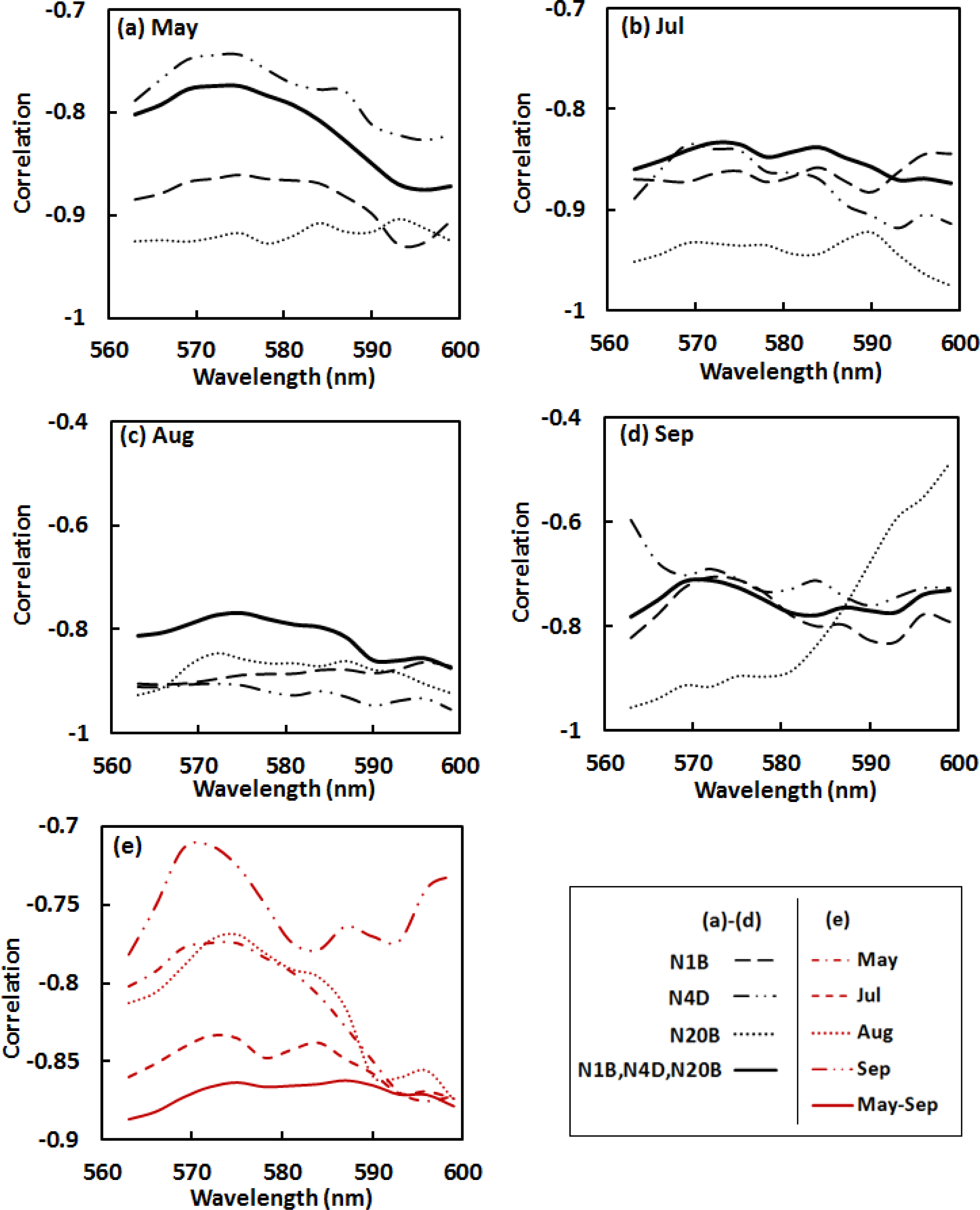
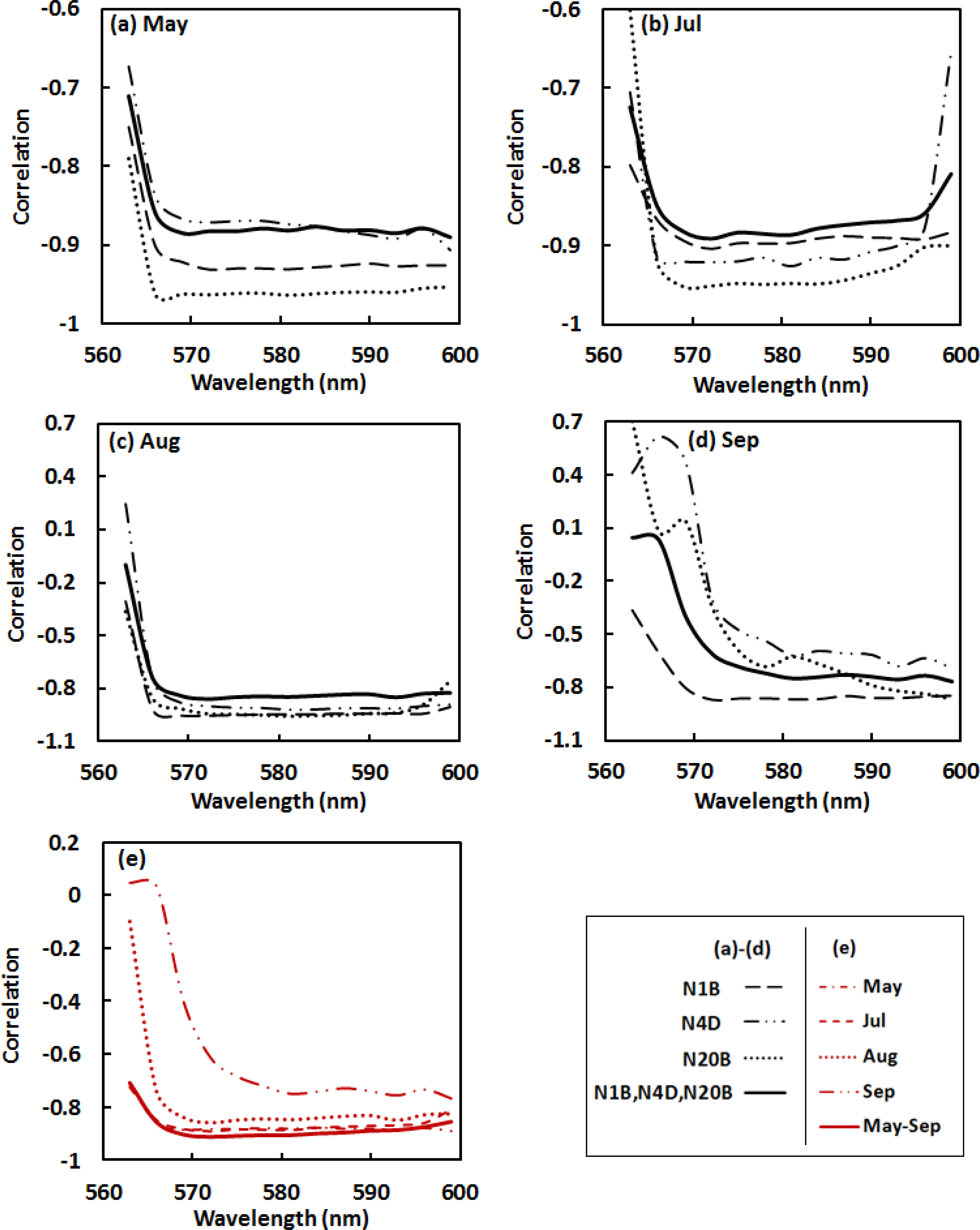
Analysis of correlations (Pearson’s r) between N_can and the various spectral indices was used to evaluate the strength of relationships between canopy N and spectral reflectance across the 562–600 nm absorption feature for each watershed individually, and for the three watersheds together. For each pooled dataset of three watersheds, thirty samples were randomly selected from the total samples of 45 in the May–August data (18 from the total 27 in September data) for correlation analysis. For the first derivative data (Figure 4), significant wavelengths related to nitrogen content included the regions from 563–566 nm and 593–596 nm, where the absolute r-values were greater than 0.75 across all watersheds and all dates. A common region with relatively low absolute r-values was at wavelengths of 569–575 nm centered at 572 nm, corresponding to the region with maximum absolute values of the first derivative data, where the original reflectance values decreased fastest. Absolute r-values for the pooled datasets (May–September) were greater than 0.86 (Figure 4e), which indicates a generally strong correlation between foliar N and the first derivative data in the given absorption spectral feature across various spatial and temporal scales.

For the continuum removed spectra (Figure 5), absolute r-values at wavelengths of 569–593 nm in May–August had a range from 0.83 to 0.89 (Figure 5a–c). Spectral region of 578–593 nm in September with the absolute r of 0.72–0.76 (Figure 5d), was strongly related to N_can across the three watersheds. Correlations between the nitrogen and the spectral dataset incorporating data for the three watersheds throughout the entire growing season were relatively strong in the region of 569–584 nm with the absolute values of r greater than 0.90 (Figure 5e).

Based on the results of the correlation analyses, absolute values of r in the region of 562–569 nm start with low ranges and vary dramatically. This can be accounted for the continuum removal line that presses close to the reflectance spectral curve at the left end of the absorption feature, resulting in highly “compressed” continuum removed values in this region (Figure 3b). It was better to exclude this region in analysis as the highly “compressed” continuum removed values reveal little useful spectral variation information. We therefore calculated the SDVI using the continuum removed spectral features at the wavelengths of 572 nm and 581 nm—CR572 and CR581. The wavelength at 572 nm is in the starting portion of the “normal” continuum removed spectral region; 581 nm is around the middle point between 562 and 600 nm, which is the nadir in the continuum removed absorption trough. Further correlation analysis supports the use of SVDI formed at these wavelengths as an indicator of canopy N, with absolute r-values between N_can and the SDVI varying from 0.78 to 0.96 (

Table 3. Correlations between canopy nitrogen N_can and the SDVI for the field-collected data.

Months	Sites	Sample Size	r
May	N1B	15	0.93
	N4D	15	0.87
	N20B	15	0.96
	N1B, N4D, N20B	30	0.88
June/July	N1B	15	0.87
	N4D	15	0.93
	N20B	15	0.94
	N1B, N4D, N20B	30	0.87
August	N1B	15	0.93
	N4D	15	0.93
	N20B	15	0.96
	N1B, N4D, N20B	30	0.83
September	N1B	12	0.85
	N4D	8	0.78
	N20B	7	0.82
	N1B, N4D, N20B	18	0.83
May–September	N1B, N4D, N20B	108	0.88

).

4.2. Canopy Nitrogen Modeling From in situ Data

Thirty samples were randomly selected from the May–August data (18 from the September data) for model development. The remaining 15 samples (nine from September) were reserved for validation. Descriptive statistics of the in situ datasets of canopy nitrogen contents for modeling and validation (

Table 4. Descriptive statistics of the in situ N_can datasets for modeling and validation.

Months	Modeling					Validation
	Sample Size	Min.	Max.	Mean	SD	Sample Size	Min.	Max.	Mean	SD
		(g·m−2)					(g·m−2)
May	30	0.64	4.18	2.11	0.89	15	0.73	3.54	2.01	0.83
June/July	30	0.62	3.48	1.90	0.73	15	0.70	3.30	1.88	0.75
August	30	0.45	2.80	1.31	0.50	15	0.46	2.22	1.24	0.45
September	18	0.36	1.17	0.68	0.25	9	0.36	1.13	0.60	0.21
May–September	108	0.36	4.18	1.59	0.84	54	0.36	3.54	1.52	0.81

) demonstrate that the ranges of the modeling datasets were in general slightly larger than that of the corresponding validation datasets, indicating that the modeling datasets cover the full range of N contents well. Similar values of the mean and standard deviation (SD) between the modeling and validation datasets suggest similar central tendencies and dispersions between the two types of datasets. This verifies a reasonable selection of modeling and validation values.

Monthly models of canopy nitrogen retrieval using hyperspectral data for May, July, August and September, and a general model for the whole growing season were derived using regression analysis. All of possible wavelength combinations were examined using the first derivative and continuum removed spectra, subject to restrictions imposed by the modeling method. Chief among these choices was to limit the number of independent variables. Although a model may fit the data better when incorporating more independent variables, an excessive number may result in an overfit model that will not perform well in validation. For our data, the need to limit model inputs is even more pronounced since the independent variables are spectral features concentrated in a narrow region, which might be strongly correlated with each other and thus might not be all statistically significant in the model. We therefore used combinations of no more than three independent variables for each model. In addition to the multivariate models based on individual spectral bands, other models were derived using only the SDVI. All of the regression models were validated by comparing the measured nitrogen from the samples reserved for validation with the values estimated using the remote sensing methods.

The best-performing models from the regression analysis are summarized in

Table 5. Regression models for canopy nitrogen recovery using field-measured derivative (D), continuum removed reflectance (CR) spectra and SDVI.

Month	Modeling				Validation
	Sample Size	Formula	R2	Adj R2	Sample Size	RMSE (g·m−2)	R2
May	30	Ncan = 2.24−27510 × D566 + 35220 × D578 − 17900 × D599	0.86	0.84	15	0.50	0.74
		Ncan = 46.64 − 442.52 × CR581 + 395.33 × CR584	0.81	0.80		0.29	0.94
		Ncan = 197.56 × SDVI	0.77	0.76		0.21	0.96
June/July	30	Ncan = 2.22 − 8171 × D563 + 18330 × D584 − 18070 × D593	0.85	0.84	15	0.35	0.79
		Ncan = 21.22 − 230.92 × CR581 + 209.85 × CR587	0.85	0.84		0.30	0.86
		Ncan = 162.16 × SDVI	0.74	0.73		0.24	0.90
August	30	Ncan = 1.55 − 24840 × D569 + 24150 × D572 − 5622 × D599	0.86	0.85	15	0.23	0.74
		Ncan = 115.57 − 155.35 × CR575 + 325.07 × CR590 − 284.87 × CR593	0.84	0.82		0.21	0.78
		Ncan = 147.57 × SDVI	0.67	0.65		0.16	0.86
September	18	Ncan = 1.40 − 8152 × D563 + 11096 × D569 − 8887 × D578	0.77	0.72	9	0.22	0.37
		Ncan = 252.02 + 83.51 × CR566 − 335.41 × CR599	0.69	0.65		0.17	0.45
		Ncan = 137.09 × SDVI	0.69	0.67		0.17	0.41
May–September	108	Ncan = 1.71 − 13570 × D566 + 14160 × D575 − 7232 × D590	0.85	0.85	54	0.28	0.89
		Ncan = 38.44 − 311.08 × CR581 + 272.56 × CR584	0.86	0.85		0.24	0.92
		Ncan = 169.73 × SDVI	0.77	0.77		0.25	0.92

. Note that while the form of the regression models remains the same, the empirical coefficients of each model changed in each month of data collection. This is hardly surprising, given the empirical nature of the modeling and the continual changes in the canopy over the growing seasons.

The coefficient of determination (R²) was generally lower for the validation data than for the model-development data. Again, this is not unexpected. The similarity of the error metrics from the model development step and the validation step suggests that the models have little overfitting and should therefore be robust when applied to new data. In general, there was little difference between the two best multivariable band-based models and the univariate SDVI model. Model performances were also similar throughout most of the growing season, although there was a notable decrease in model performance in September. This result could be due to differences in canopy phenology. At the time of the September data collection the canopy was beginning to senesce, so the fraction of green material in the canopy was likely less than in the previous data collection periods. It could also be an artifact of the smaller sample size, which resulted in a validation set with samples size = 9.

The results from pooling all the data (May–September) were similar to, and in some cases better than, the results from the individual months. This is a particularly important outcome, since it suggests that one model may be sufficient to predict N_can across the entire growing season, eliminating the need to use multiple models depending on the growth state of the canopy. The larger sample size available for both model development and validation (the result of combining all of the measurements) might also explain some of the better validation results in the pooled sample.

4.3. Canopy Nitrogen Retrieval from Airborne Imagery

Results from the in situ spectrometry (Sections 4.1 and 4.2) suggest that SDVI calculated using continuum removed reflectance in the spectral region of 562–600 nm yielded the best model for retrieving N_can. While the validation metrics for the SDVI model differed little from the multivariate models, the intrinsic parsimony of the SDVI model (because it is based on a single independent variable) strongly support its further use in N_can retrieval models. However, we chose to analyze the data from the aerial imagery as we did the in situ data. Here, we tested all forms of retrieval model in order to confirm if SDVI still yielded the best prediction models when applied to a data set with different spatial and spectral resolution. We therefore repeated the analysis described in Section 4.2, using the atmospherically corrected reflectance data collected during the four aircraft overflights.

Results of modeling and validation for nitrogen retrieval from airborne imagery (

Table 6. Regression models for canopy nitrogen retrieval using derivative (D), continuum removed reflectance (CR) spectra and SDVI derived from aircraft image.

Month	Modeling				Validation
	Sample Size	Formula	R2	Adj R2	Sample Size	RMSE (g·m−2)	R2
May	30	Ncan = 2.15 + 6267.42 × D567 − 4594.36 × D578 − 5714.14 × D599	0.84	0.82	15	0.23	0.85
		Ncan = 47.88 − 48.50 × CR583	0.87	0.86		0.21	0.86
		Ncan = 113.47 × SDVI	0.84	0.83		0.24	0.82
June/July	30	Ncan = 2.45 − 6392 × D595	0.72	0.72	15	0.23	0.82
		Ncan = 53.37 − 54.67 × CR583	0.67	0.66		0.25	0.69
		Ncan = 118.37 × SDVI	0.59	0.58		0.16	0.79
August	30	Ncan = 0.67 − 4597.39 × D564 + 2819.05 × D578 − 1013.86 × D597	0.93	0.92	15	0.20	0.63
		Ncan = 55.58 − 56.50 × CR574	0.83	0.83		0.15	0.75
		Ncan = − 0.48 + 109.11 × SDVI	0.76	0.75		0.18	0.74
September	18	Ncan = 1.01 − 2522 × D582	0.67	0.65	9	0.09	0.80
		Ncan = 72.75 × CR572 − 72.42 × CR582	0.59	0.56		0.19	0.44
		Ncan = 0.33 + 141.62 × SDVI	0.58	0.56		0.19	0.45
May–August	90	Ncan = 1.40 − 2699 × D583 − 1094 × D592	0.81	0.80	45	0.22	0.86
		Ncan = 42.90 − 46.72 × CR569 − 174.86 × CR585 + 178.43 × CR588	0.84	0.83		0.24	0.84
		Ncan = − 0.33 + 125.38 × SDVI	0.60	0.60		0.32	0.67

) showed that reasonably accurate N_can estimation models can be determined from datasets of either the first derivative and continuum removed reflectance or the SDVI values. Feasible models for September suggested that the wider spectral bands (10 nm vs. 3 nm, see Section 3.1) were still adequate for nitrogen estimates. Despite variations in selection of wavelength combinations for optimal nitrogen modeling in different months, general nitrogen retrieval models could be developed for the growth seasons during May–August.

The models developed from the first derivative and the continuum removed spectral data showed higher R² values for regression modeling and lower ranges of RMSE for model validation than the SDVI model, indicating that multivariate models performed better for the canopy N estimates based on the aircraft data. As with the in situ data, there was little difference between the accuracy of each month’s model and the overall accuracy of the pooled (all-months) models. Again, this is a significant result, as it shows that N_can can be extracted across the growing season using the same retrieval model, simplifying the processing of data collected at various times during the growing seasons.

4.4. Comparison of Results and Nitrogen Mapping using Aerial Imagery

Even though the in situ data were resampled with similar band passes to the aerial imagery, differences in other physical mechanisms and measurement conditions between the two sensors possibly make it still difficult for the two sets of measurements to be interchangeable. Wavelength combinations and empirical model coefficients vary between optimal in situ models and the corresponding aerial imagery models. This is not unexpected given the intrinsic features of empirical methods. However, similar results of model performance and validation suggest that these methods are feasible and stable when applied to respective datasets of field spectra and aerial imagery. In other words, the field model is applicable to the field data, and the aircraft model to the aircraft data, but the two cannot be interchanged.

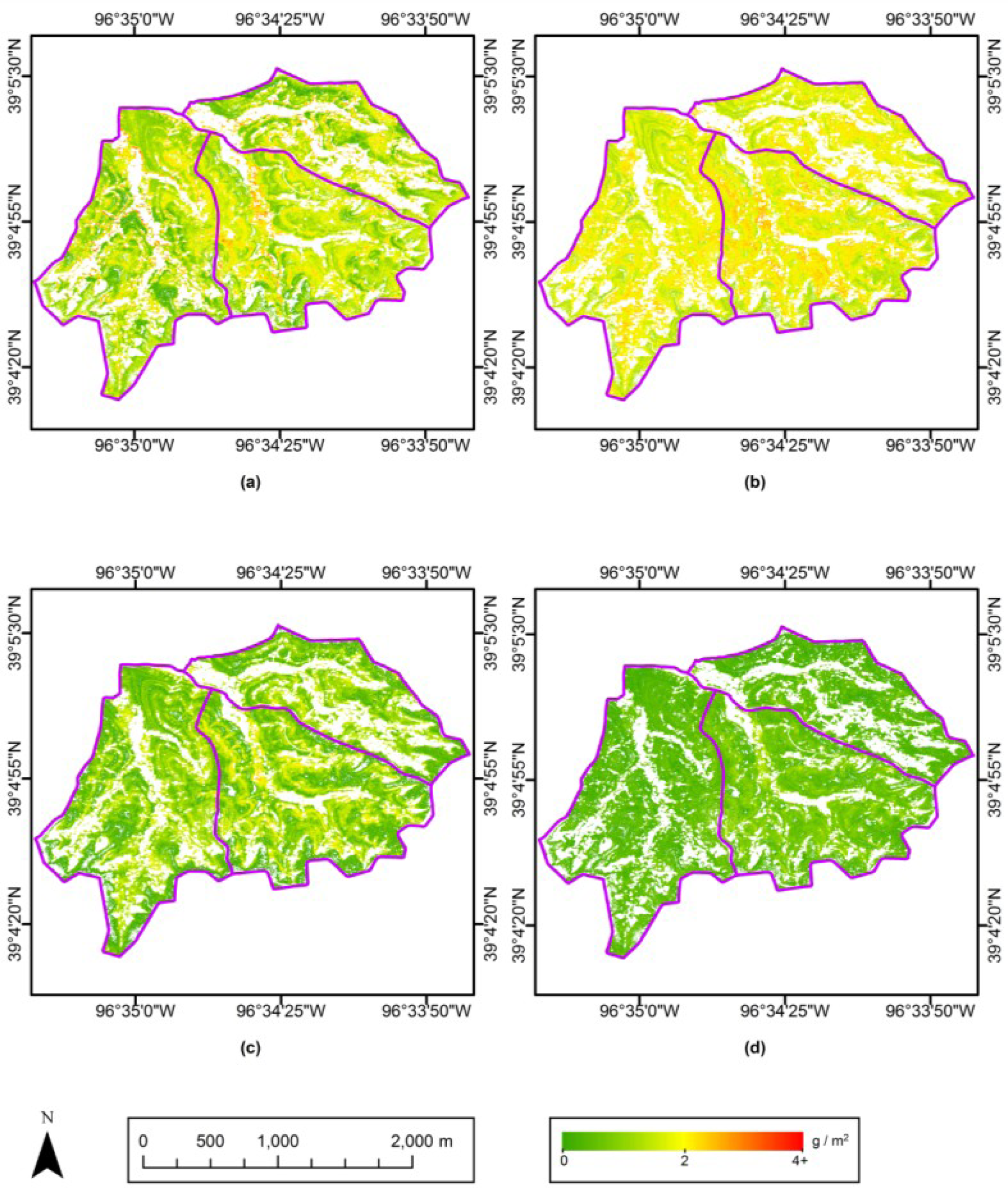
Maps of N_can for the entire study site were made using the best-performing equation among the pooled retrieval models. Because the pooled model developed from the first derivative of spectral reflectance at 583 and 592 nm had the lowest RMSE, we used it to create maps of N_can for May–August (Figure 6a–c). The N_can map for September was created using the first derivative at 582 nm due to the different spectral resolution of aerial imagery in September (Figure 6d). These N_can maps support the statistical comparison across various spatial and temporal scales (Table 2 in Section 4.1), and also provide more spatial detail and phenological characteristics.

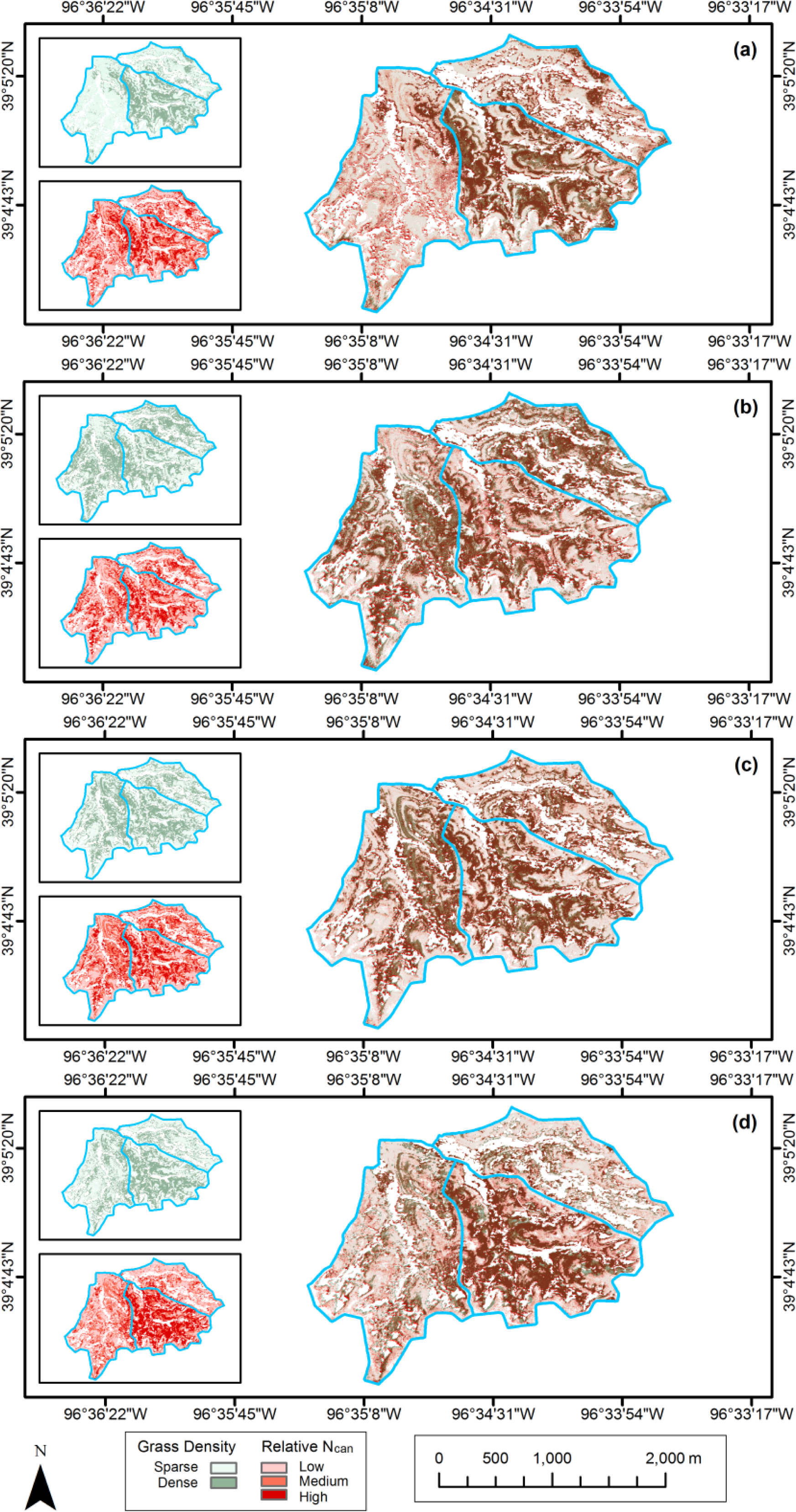
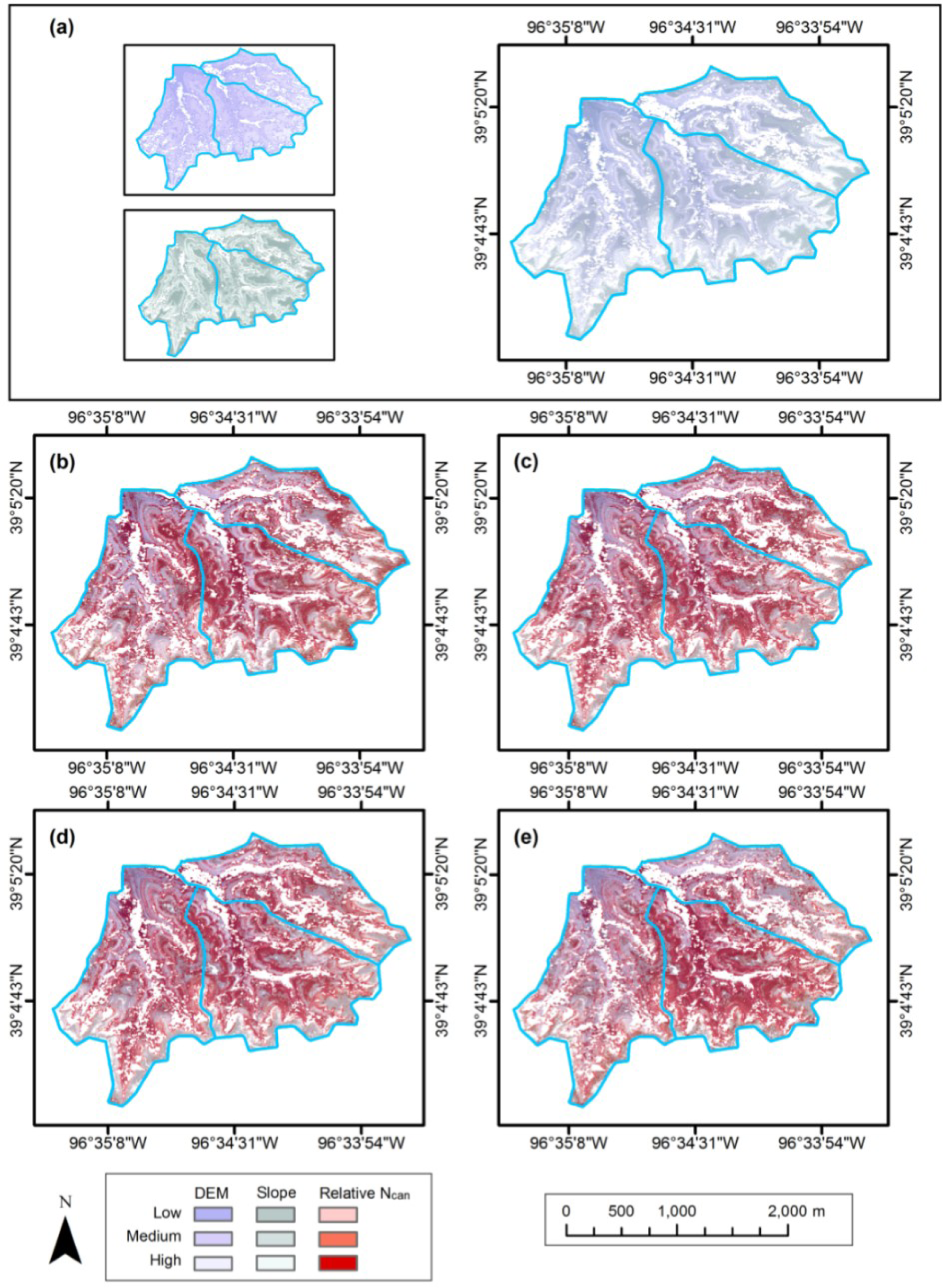
4.5. Assessment of N Relation to Fire, Vegetation Density and Topography

The patterns in the N_can maps were expected to be affected by fire frequency, vegetation density and topography over the study site. To evaluate these influences on N_can distribution, N_can estimations on each map were stratified into the low, medium and high levels by 3-quantiles, and then compared to the land cover type (sparse grasses vs. dense grasses, classified by supervised Maximum Likelihood in Section 3.2.3) and a digital elevation model (DEM, with spatial resolution of 2 m × 2 m) [56]. The effect of fire frequency can be seen in the N_can stratifications between watersheds (Figure 7). N_can values in watershed N1B with fire frequency of one year are generally higher than in the other two watersheds. This is especially noticeable in the May and September imagery, where the effects of canopy and treatment heterogeneity are most prominent. The July image shows relatively even distribution of N_can, consistent with a period in which the canopy is more uniformly green and actively photosynthesizing.

The spatial relationships between N_can, canopy density and topography observed in the three watersheds of our study (Figures 7 and 8) are fairly straightforward, similar to those observed throughout KPBS [57]. Values of N_can coincide directly with canopy density. Canopy density, in turn, is closely related to topography through its effect on soil thickness and moisture. The densest canopies are found in flatter, low-lying areas, where the soil depth is greatest and soil moisture tends to be highest. Thinnest canopies occur on hill sides, where slope is greatest and the thin, rocky soil layer is unable to retain the moisture needed to support a denser canopy. Intermediately thick canopies occur mainly on hilltops, drainage divides, and other topographic highs, where slopes are low and soils depths are greater than on slope sides but less than in the bottom areas. This topographic effect on N_can distribution is most noticeable in May, but becomes less so as the canopies become more developed during the growing seasons.

5. Conclusions

Our results show that canopy nitrogen can be estimated using empirical models based on hyperspectral remote sensing data collected from a tallgrass prairie canopy subjected to varying fire treatments and characterized by a heterogeneous mix of species and canopy structures. Spectra collected from both ground-based and aircraft-mounted spectroradiometers were used to develop empirical retrieval models. A simple model based on the SDVI was best for estimating N_can from the ground-based data, whereas a multivariate regression model performed best using the aircraft data. However, the differences between the models were small, and in general models from both data types were comparably accurate.

Comparing our results with similar studies recorded in the literature suggests that the performance metrics for our best empirical models were generally comparable to those of similar analyses conducted over other canopy types. In past efforts, remote estimation of canopy N content yielded the best results when applied to agricultural ecosystems of various types [35,58–60]. This is perhaps to be expected. Although crop canopies are not simple monocultures they are more homogeneous than most natural vegetation canopies and therefore present a more uniform surface from which to extract biophysical information. Forest canopies, a natural surface but one typically characterized by a less diverse range of species actually visible to the sensor, also tended to provide slightly better results in remote analysis of nitrogen when compared to ours [61–63]. Among those studies done in grasslands or other more heterogeneous environments, our results were quite similar to those reported by Boegh et al. [64]—a study in which the problem of canopy heterogeneity was considered directly—and to those reported by Asner et al. [13], Kooistra et al. [65], and Mitchell et al. [66].

While our results agree with and support previous work on retrieving canopy biochemical concentrations via remote sensing, there are also findings of further relevance. Most importantly, our results show that empirical methods for N retrieval can be robust when applied to a canopy with both spatial and temporal heterogeneity. In this case, the spatial heterogeneity was introduced as part of the research protocol by including three experimental units (i.e., watersheds) whose differing burn treatments yield very different canopy conditions. In addition, all three of these watersheds studied here were subjected to grazing by large ungulates, further contributing to a diverse and complex canopy. For each month of data collection, the same empirical model was able to estimate N_can in each watershed with comparable accuracy. This is a significant result since it shows that N_can (and possibly other elements of stoichiometric interests) can be mapped across diverse canopies without the need for stratification and the use of multiple models. In addition, our results show that empirical models can perform well across the entire growing season, again obviating the need for multiple empirical models calibrated to account for phenology.

References

- Focardi, S.; Marcellini, P.; Montanaro, P. Do ungulates exhibit a food density threshold? A study of optimal foraging and movement patterns. J. Anim. Ecol 1996, 65, 606–620. [Google Scholar]
- Jaramillo, V.J.; Detling, J.K. Grazing history, defoliation, and competition: Effects on shortgrass production and nitrogen accumulation. Ecology 1988, 69, 1599–1608. [Google Scholar]
- Post, E.S.; Klein, D.R. Relationships between graminoid growth form and levels of grazing by Caribou (Rangifer tarandus) in Alaska. Oecologia 1996, 107, 364–372. [Google Scholar]
- Schimel, D.; Parton, W.; Adamsen, F.; Woodmansee, R.; Senft, R.; Stillwell, M. The role of cattle in the volatile loss of nitrogen from a shortgrass steppe. Biogeochemistry 1986, 2, 39–52. [Google Scholar]
- Sala, O.E. Temperate Grasslands. In Global Biodiversity in a Changing Environment: Scenarios for the 21st Century; Chapin, F.S., III, Sala, O.E., Huber-Sannvald, E., Eds.; Springer: New York, NY, USA, 2001; pp. 121–137. [Google Scholar]
- Samson, F.B.; Knopf, F.L. Prairie Conservation: Preserving North America’s Most Endangered Ecosystem; Island Press: Washington, DC, USA, 1996. [Google Scholar]
- Hobbs, N.T.; Schimel, D.S.; Owensby, C.E.; Ojima, D. Fire and grazing in the tallgrass prairie: Contingent effects on nitrogen budgets. Ecology 1991, 72, 1374–1382. [Google Scholar]
- Fuhlendorf, S.D.; Engle, D.M. Restoring heterogeneity on rangelands: Ecosystem management based on evolutionary grazing patterns. Bioscience 2001, 51, 625–632. [Google Scholar]
- Whiles, M.R.; Charleton, R.E. The ecological significance of tallgrass prairie arthropods. Annu. Rev. Entomol 2006, 51, 387–412. [Google Scholar]
- Archibald, S.; Bond, W.; Stock, W.; Fairbanks, D. Shaping the landscape: Fire-grazer interactions in an African savanna. Ecol. Appl 2005, 15, 96–109. [Google Scholar]
- Mueller, T.; Olson, K.A.; Fuller, T.K.; Schaller, G.B.; Murray, M.G.; Leimgruber, P. In search of forage: Predicting dynamic habitats of Mongolian gazelles using satellite-based estimates of vegetation productivity. J. Appl. Ecol 2008, 45, 649–658. [Google Scholar]
- Bernhard, A. The nitrogen cycle: Processes, players, and human impact. Natl. Educ. Knowl 2010, 3, 25. [Google Scholar]
- Asner, G.P.; Wessman, C.A.; Bateson, C.; Privette, J.L. Impact of tissue, canopy, and landscape factors on the hyperspectral reflectance variability of arid ecosystems. Remote Sens. Environ 2000, 74, 69–84. [Google Scholar]
- Richards, J.A.; Jia, X. Remote Sensing Digital Image Analysis: An Introduction; Springer: New York, NY, USA, 2006. [Google Scholar]
- Knyazikhin, Y.; Schull, M.A.; Stenberg, P.; Mõttus, M.; Rautiainen, M.; Yang, Y.; Marshak, A.; Carmona, P.L.; Kaufmann, R.K.; Lewis, P.; et al. Hyperspectral remote sensing of foliar nitrogen content. Proc. Natl. Acad. Sci. USA 2013, 110, E185–E192. [Google Scholar]
- Sembiring, H.; Raun, W.R.; Johnson, G.V.; Stone, M.L.; Solie, J.B.; Phillips, S.B. Detection of nitrogen and phosphorus nutrient status in Bermudagrass using spectral radiance. J. Plant Nutr 1998, 21, 1189–1206. [Google Scholar]
- Peñuelas, J.; Gamon, J.A.; Fredeen, A.L.; Merino, J.; Field, C.B. Reflectance indices associated with physiological changes in nitrogen and water-limited sunflower leaves. Remote Sens. Environ 1994, 48, 135–146. [Google Scholar]
- Zhang, C.; Kovacs, J.M.; Wachowiak, M.P.; Flores-Verdugo, F. Relationship between hyperspectral measurements and mangrove leaf nitrogen concentrations. Remote Sens 2013, 5, 891–908. [Google Scholar]
- Gates, D.M.; Keegan, H.J.; Schleter, J.C.; Weidner, V.R. Spectral properties of plants. Appl. Opt 1965, 4, 11–20. [Google Scholar]
- Curran, P.J. Remote sensing of foliar chemistry. Remote Sens. Environ 1989, 30, 271–278. [Google Scholar]
- Kokaly, R.F. Investigating a physical basis for spectroscopic estimates of leaf nitrogen concentration. Remote Sens. Environ 2001, 75, 153–161. [Google Scholar]
- Curran, P.J.; Dungan, J.L.; Peterson, D.L. Estimating the foliar biochemical concentration of leaves with reflectance spectrometry: Testing Kokaly and Clark methodologies. Remote Sens. Environ 2001, 76, 349–359. [Google Scholar]
- Jago, R.A.; Cutler, M.E.J.; Curran, P.J. Estimating canopy chlorophyll concentration from field and airborne spectra. Remote Sens. Environ 1999, 68, 217–224. [Google Scholar]
- Martin, M.E.; Aber, J.D. High spectral resolution remote sensing of forest canopy lignin, nitrogen, and ecosystem processes. Ecol. Appl 1997, 7, 431–443. [Google Scholar]
- Mutanga, O.; Skidmore, A.K.; Kumar, L.; Ferwerda, J.G. Estimating tropical pasture quality at canopy level using band depth analysis with continuum removal in the visible domain. Int. J. Remote Sens 2005, 26, 1093–1108. [Google Scholar]
- Yoder, B.J.; Pettigrew-Crosby, R.E. Predicting nitrogen and chlorophyll content and concentrations from reflectance spectra (400–2500 nm) at leaf and canopy scales. Remote Sens. Environ 1995, 53, 199–211. [Google Scholar]
- Ferwerda, J.G.; Skidmore, A.K.; Mutanga, O. Nitrogen detection with hyperspectral normalized ratio indices across multiple plant species. Int. J. Remote Sens 2005, 26, 4083–4095. [Google Scholar]
- Kawamura, K.; Watanabe, N.; Sakanoue, S.; Inoue, Y. Estimating forage biomass and quality in a mixed sown pasture based on partial least squares regression with waveband selection. Grassl. Sci 2008, 54, 131–145. [Google Scholar]
- Kokaly, R.F.; Clark, R.N. Spectroscopic determination of leaf biochemistry using band-depth analysis of absorption features and stepwise multiple linear regression. Remote Sens. Environ 1999, 67, 267–287. [Google Scholar]
- Kokaly, R.F.; Despain, D.G.; Clark, R.N.; Livo, K.E. Mapping vegetation in Yellowstone National Park using spectral feature analysis of AVIRIS data. Remote Sens. Environ 2003, 84, 437–456. [Google Scholar]
- Laba, M.; Tsai, F.; Ogurcak, D.; Smith, S.; Richmond, M.E. Field determination of the optimal dates for the discrimination of invasive wetland plant species using derivative spectral analysis. Photogramm. Eng. Remote Sens 2005, 71, 603–611. [Google Scholar]
- Mutanga, O.; Skidmore, A.K.; Prins, H.H.T. Discriminating sodium concentration in a mixed grass species environment of the Kruger National Park using field spectrometry. Int. J. Remote Sens 2004, 25, 4191–4201. [Google Scholar]
- Daughtry, C.S.T.; Walthall, C.L.; Kim, M.S.; de Colstoun, E.B.; McMurtrey, J.E., III. Estimating corn leaf chlorophyll concentration from leaf and canopy reflectance. Remote Sens. Environ 2000, 74, 229–239. [Google Scholar]
- Sims, D.A.; Gamon, J.A. Relationships between leaf pigment content and spectral reflectance across a wide range of species, leaf structures and developmental stages. Remote Sens. Environ 2002, 81, 337–354. [Google Scholar]
- Wu, C.; Niu, Z.; Tang, Q.; Huang, W. Estimating chlorophyll content from hyperspectral vegetation indices: Modeling and validation. Agric. Forest Meteorol 2008, 148, 1230–1241. [Google Scholar]
- Delalieux, S.; Somers, B.; Verstraeten, W.W.; Keulemans, W.; Coppin, P. Hyperspectral canopy measurements under artificial illumination. Int. J. Remote Sens 2008, 29, 6051–6058. [Google Scholar]
- Allred, B.W.; Fuhlendorf, S.D.; Engle, D.M.; Elmore, R.D. Ungulate preference for burned patches reveals strength of fire-grazing interaction. Ecol. Evol 2011, 1, 132–144. [Google Scholar]
- Collins, S.L.; Calabrese, L.B. Effects of fire, grazing and topographic variation on vegetation structure in tallgrass prairie. J. Veg. Sci 2012, 23, 563–575. [Google Scholar]
- Collins, S.L.; Knapp, A.K.; Briggs, J.M.; Blair, J.M.; Steinauer, E.M. Modulation of diversity by grazing and mowing in native tallgrass prairie. Science 1998, 280, 745–747. [Google Scholar]
- Seagle, S.W.; McNaughton, S. Spatial variation in forage nutrient concentrations and the distribution of Serengeti grazing ungulates. Landsc. Ecol 1992, 7, 229–241. [Google Scholar]
- Wilmshurst, J.F.; Fryxell, J.M.; Hudsonb, R.J. Forage quality and patch choice by wapiti (Cervus elaphus). Behav. Ecol 1995, 6, 209–217. [Google Scholar]
- McNaughton, S.J. Compensatory plant growth as a response to herbivory. Oikos 1983, 40, 329–336. [Google Scholar]
- Anderson, T.M.; Ritchie, M.E.; Mayemba, E.; Eby, S.; Grace, J.B.; McNaughton, S.J. Forage nutritive quality in the Serengeti ecosystem: The roles of fire and herbivory. Am. Nat 2007, 170, 343–357. [Google Scholar]
- Risser, P.G.; Birney, E.C.; Blocker, H.D.; May, S.W.; Parton, W.J.; Wiens, J.A. The True Prairie Ecosystem; Hutchinson Ross Publishing Company: Stroudsburg, PA, USA, 1981. [Google Scholar]
- Knapp, A.K.; Briggs, J.M.; Hartnett, D.C.; Collins, S.L. Grassland Dynamics: Long-Term Ecological Research in Tallgrass Prairie; Oxford Press: New York, NY, USA, 1998. [Google Scholar]
- Hartnett, D.C.; Hickman, K.R.; Walter, L.E.F. Effects of bison grazing, fire, and topography on floristic diversity in tallgrass prairie. J Range Manag 1996, 49, 413–420. [Google Scholar]
- Wallace, L.L.; Turner, M.G.; Romme, W.H.; Oneill, R.V.; Wu, Y.G. Scale of heterogeneity of forage production and winter foraging by elk and bison. Landsc. Ecol 1995, 10, 75–83. [Google Scholar]
- Schuler, K.L.; Leslie, D.M.; Shaw, J.H.; Maichak, E.J. Temporal-spatial distribution of American bison (Bison bison) in a tallgrass prairie fire mosaic. J. Mammal 2006, 87, 539–544. [Google Scholar]
- Yin, X.; Latinga, E.A.; Schapendonk, A.H.; Zhong, X. Some quantitative relationships between leaf area index and canopy nitrogen content and distribution. Ann. Bot 2003, 91, 893–903. [Google Scholar]
- Efron, B.; Gong, G. A leisurely look at the bootstrap, the jackknife, and cross-validation. Am. Stat 1983, 37, 36–48. [Google Scholar]
- Blackburn, G.A. Hyperspectral remote sensing of plant pigments. J. Exp. Bot 2007, 58, 855–867. [Google Scholar]
- Cater, G.A.; Knapp, A.K. Leaf optical properties in higher plants: Linking spectral characteristics to stress and chlorophyll concentration. Am. J. Bot 2001, 88, 677–684. [Google Scholar]
- Van den Berg, A.K.; Perkins, T.D. Evaluation of a portable chlorophyll meter to estimate chlorophyll and nitrogen contents in sugar maple (Acer saccharum Marsh.) leaves. For. Ecol. Manag 2004, 200, 113–117. [Google Scholar]
- Rodriguez, I.R.; Miller, G.L. Using a chlorophyll meter to determine the chlorophyll concentration, nitrogen concentration, and visual quality of St. Augustinegrass. HortScience 2000, 35, 751–754. [Google Scholar]
- Myneni, R.B.; Williams, D.L. On the relationship between FAPAR and NDVI. Remote Sens. Environ 1994, 49, 200–211. [Google Scholar]
- Konza Prairie LTER. Available online: http://www.konza.ksu.edu/knz/pages/data/GISdata.aspx (accessed on 9 March 2014).
- Hartnett, D.C.; Fay, P.A. Plant Populations: Patterns and Processes. In Grassland Dynamics: Long-Term Ecological Research in Tallgrass Prairie; Knapp, A.K., Briggs, J.M., Hartnett, D.C., Collins, S.L., Eds.; Oxford Press: New York, NY, USA, 1998; pp. 81–100. [Google Scholar]
- Inoue, Y.; Sakaiya, E.; Zhu, Y.; Takahashi, W. Diagnostic mapping of canopy nitrogen content in rice based on hyperspectral measurements. Remote Sens. Environ 2012, 126, 210–221. [Google Scholar]
- Tilling, A.K.; O’Leary, G.J.; Ferwerda, J.G.; Jones, S.D.; Fitzgerald, G.J.; Rodriguez, D.; Belford, R. Remote sensing of nitrogen and water stress in wheat. Field Crop. Res 2007, 104, 77–85. [Google Scholar]
- Yi, Q.; Huang, J.; Wang, F.; Wang, X. Quantifying biochemical variables of corn by hyperspectral reflectance at leaf scale. J. Zhejiang Univ. Sci B 2008, 9, 378–384. [Google Scholar]
- Peterson, D.L.; Aber, J.D.; Matson, P.A.; Card, D.H.; Swanberg, N.; Wessman, C.; Spanner, M. Remote sensing of forest canopy and leaf biochemical contents. Remote Sens. Environ 1988, 24, 85–108. [Google Scholar]
- Smith, M.-L.; Ollinger, S.V.; Martin, M.E.; Aber, J.D.; Hallett, R.A.; Goodale, C.L. Direct estimation of aboveground forest productivity through hyperspectral remote sensing of canopy nitrogen. Ecol. Appl 2002, 12, 1286–1302. [Google Scholar]
- Wessman, C.A.; Aber, J.D.; Peterson, D.L.; Melillo, J.M. Remote sensing of canopy chemistry and nitrogen cycling in temperate forest ecosystems. Nature 1988, 335, 154–156. [Google Scholar]
- Boegh, E.; Houborg, R.; Bienkowski, J.; Braben, C.F.; Dalgaard, T.; van Dijk, N.; Dragosits, U.; Holmes, E.; Magliulo, V.; Schelde, K.; et al. Remote sensing of LAI, chlorophyll, and leaf nitrogen pools of crop- and grasslands in five European landscapes. Biogeosciences 2012, 9, 10149–10205. [Google Scholar]
- Kooistra, L.; Roelofsen, H.; Wamelink, G.W.W.; Witte, J.P.M.; Clevers, J.G.P.W. Assessment of the Biomass and Nitrogen Status of Natural Grasslands Using Hyperspectral Remote Sensing. Proceedings of the Hyperspectral 2010 Workshop (SP-683), Frascati, Italy, 17–19 March 2010; Available online: http://earth.esa.int/workshops/hyperspectral_2010/papers/s5_7koois.pdf (accessed on 9 May 2014).
- Mitchell, J.J.; Glenn, N.F.; Sankey, T.T.; Derryberry, D.R.; Germino, M.J. Remote sensing of sagebrush canopy nitrogen. Remote Sens. Environ 2012, 124, 217–223. [Google Scholar]