Article

Pan-Arctic Climate and Land Cover Trends Derived from Multi-Variate and Multi-Scale Analyses (1981–2012)

1
Department for Earth Observation, Friedrich-Schiller-University, Jena 07743, Germany
2
Department for Biochemical Integration, Max-Planck-Institute for Biogeochemistry, Jena 07745, Germany
3
Centre for Geo-Information, Wageningen University, Wageningen 6700AA, The Netherlands
*
Author to whom correspondence should be addressed.
Remote Sens. 2014, 6(3), 2296-2316; https://doi.org/10.3390/rs6032296
Submission received: 22 November 2013 / Revised: 19 February 2014 / Accepted: 5 March 2014 / Published: 12 March 2014
(This article belongs to the Special Issue Remote Sensing of Changing Northern High Latitude Ecosystems)

Abstract

:
Arctic ecosystems have been afflicted by vast changes in recent decades. Changes in temperature, as well as precipitation, are having an impact on snow cover, vegetation productivity and coverage, vegetation seasonality, surface albedo, and permafrost dynamics. The coupled climate-vegetation change in the arctic is thought to be a positive feedback in the Earth system, which can potentially further accelerate global warming. This study focuses on the co-occurrence of temperature, precipitation, snow cover, and vegetation greenness trends between 1981 and 2012 in the pan-arctic region based on coarse resolution climate and remote sensing data, as well as ground stations. Precipitation significantly increased during summer and fall. Temperature had the strongest increase during the winter months (twice than during the summer months). The snow water equivalent had the highest trends during the transition seasons of the year. Vegetation greenness trends are characterized by a constant increase during the vegetation-growing period. High spatial resolution remote sensing data were utilized to map structural vegetation changes between 1973 and 2012 for a selected test region in Northern Siberia. An intensification of woody vegetation cover at the taiga-tundra transition area was found. The observed co-occurrence of climatic and ecosystem changes is an example of the multi-scale feedbacks in the arctic ecosystems.

1. Introduction

The high latitude regions of the northern hemisphere have been undergoing significant changes during the last few decades [14]. The arctic regions are highly vulnerable to modifications in the climate system and are influenced by changes in temperature and precipitation regimes, as well as snow and vegetation dynamics. Temperature conditions in the arctic regions have never been as high, compared to the last 300 years [1]. Predictions from climate models forecast a significant increase in temperature for the upcoming decades [5]. These climate trends cause modifications in permafrost soil temperatures, snow cover dynamics, sea ice concentration, vegetation growth, and phenological dynamics [69]. Among other factors, the increasing greenhouse gas emissions from melting permafrost, as well as the recruitment of woody vegetation species to the northernmost regions are assumed to result in positive feedback mechanisms within the global climate system [1017].
The arctic regions are highly vulnerable to climate modifications, therefore the monitoring of land cover changes and triggers are of major importance. Changes in snow cover and sea ice extent have been found to have a critical impact on the environmental and ecological dynamics of the Arctic [6,18,19]. In addition to an increase in phenological activity, woody cover vegetation types, which are representing not only trees but also shrubs, have been identified to be expending in the tundra regions [2022]. Recent publications have emphasized the increase of shrub cover in the pan-arctic area [2124]. These changes in vegetation dynamics and structure are indicators for present modifications in the arctic climate system [23,2527], leading to an alternation of the energy budget, the storage capacity, as well as the permafrost dynamics on regional and global scales. The transition zone between the taiga and the tundra has an extent of nearly 13,000 km around the northern hemisphere and is of high importance in climate change studies and climate modeling [28,29]. The identification and interpretation of changes in structure, composition and dynamics of different arctic vegetation types, particularly the arctic tree line region, have been highly accentuated in scientific studies during the last decade [1,30,31]. The potential for using different earth observation data to monitor the vegetation changes at the taiga-tundra transition zone in northern Siberia has been shown by [28,32,33].
A consistent and operational monitoring of climate variables within the arctic regions is of high importance. Because information from in situ measurements is rare in the arctic regions, remote sensing investigation is a useful tool to observe and monitor various essential climate parameters. Long time series on coarse spatial resolution as well as high-resolution remote sensing data for climate research are of high importance. Hence, synergetic multi-scale methodologies for the identification and the analysis of climate parameters derived by Earth observation techniques are required. Various methods for the extraction of trends from time series data are available. A common approach is to calculate linear regressions on time series at different temporal resolutions. The majority of recent trend analyses are based on seasonal and yearly time steps. Trend analyses using monthly resolution time steps, which emphasize the variability within the yearly cycle, are underrepresented in climate change related studies. This paper focuses on the trend analysis from different climate and ecosystem parameters for monthly time series.
However, the changes and trend patterns are not homogeneous over the pan-arctic region. The aim of this paper is to show the variability of findings in temporal and spatial scale for the last 30 years using coarse resolution remote sensing data and additional products. Furthermore, high-resolution Earth observation data, from Landsat and RapidEye, are utilized to measure woody vegetation cover and vegetation structures for a 40-year time span for a selected test region in Siberia. The objectives are to (1) identify areas showing the most significant trends and dynamics, (2) analyze the co-occurrence of different climate and ecosystem parameters, as well as (3) show the synergetic potential of identifying effects of large-scale trend patterns to local scale change. This paper presents monthly trend calculation from maximum snow water equivalent (SWEmax), temperature (CRUTemp), precipitation (CRUPrecip), and NDVI (Normalized Difference Vegetation Index—NDVI3g) for the time period of 1981 to 2012. The analysis was done by identifying trend regions using a monthly temporal resolution on pan-arctic scale. A regionalization of the trend findings was done using a biodiversity map defined by the CAFF (Conservation of Arctic Flora and Fauna) [34]. On a local scale, high-resolution remote sensing data were investigated, using Landsat (1973) and RapidEye (2012) data to monitor woody vegetation cover changes between a 40 year time span at the taiga tundra transition area of the Taymyr peninsula.

2. Data and Methods

2.1. Maximum Snow Water Equivalent—ESA DUE GlobSnow

The GlobSnow program is a Data User Element (DUE) funded by the European Space Agency (ESA). This project provides information on different snow parameters in near real time, such as snow extent (SE) and snow water equivalent (SWE) for the northern hemisphere. The SWE product covers the time period since 1978 and has a spatial resolution of 25 km in EASE-Grid projection (Equal-Area Scalable Earth Grid). The product is available in daily, weekly and monthly resolutions. In this study, SWEmax information has been used for the time series trend analysis. The SWEmax information is extracted from the weekly aggregated products [35].
The SWE product is derived using remote sensing data from the Scanning Multichannel Microwave Radiometer (SMMR), Special Sensor Microwave/Imager (SSM/I), and Advanced Microwave Scanning Radiometer (AMSR-E). SMMR onboard of the Nimbus-7 satellite covers the time period from 1978 to 1987, SSM/I from 1987 to 2002, and AMSR-E, which is onboard Aqua, since 2002. Additional information about the product development and algorithms, which were used to derive SE and SWE can be found in [36]. Individual studies assessing the quality of the GlobSnow data have proven the good quality of the product with error margins below 40 mm, especially for the derivation of peak accumulation information and seasonal snow dynamics [37,38]

2.2. Temperature and Precipitation—Climate Research Unit (CRU)

For this study temperature and precipitation measurements from the Climate Research Unit (CRU TS3.2) were utilized [39]. The CRUs provide global gridded information of different climate parameters, such as temperature, precipitation, vapor pressure, cloud cover, etc., which were interpolated from meteorological stations. The input data, derived from climate stations, are collected from different archives coordinated by the World Meteorological Organization (WMO), the National Oceanographic and Atmospheric Administration (NOAA), as well as other data sources [40]. In total, the CRUs are based on data from more than 4000 meteorological stations, which are distributed around the globe. However, the amount of meteorological stations in the arctic regions is limited. The interpolation between these stations might introduce additional errors and need to be taken into account. Based on user requirements from the climatology modeling community, the spatial resolution of the products are defined with 0.5° in latitude and longitude. The time series starts in 1901. Until the early 1980s, the amount of stations has substantially increased [40,41]. Temperature and precipitation information from the CRU data archive have been widely used for arctic research studies [4245].

2.3. NDVI3g—GIMMS

The GIMMS NDVI dataset (Global Inventory Modeling and Mapping Studies—Normalized Difference Vegetation Index) from NOAA AVHRR (National Oceanic and Atmospheric Administration—Advanced Very High Resolution Radiometer) have been used in many arctic related climate studies [7,27,4652]. A new version (NDVI3g) of the long-term time series of GIMMS is available. The GIMMS NDVI3g was re-calibrated for improved usage in high-latitude regions [16,53]. The dataset covers the time period from July 1981 until December 2011 with a bi-weekly temporal and 8 km spatial resolution. The NOAA satellites are affected by the orbital drift, which causes a delay in overflying time during the life-time of each satellite [54,55]. These effects have been substantially reduced in the dataset [46,56].
As the high latitude regions are affected by snow and cloud cover, the GIMMS NDVI3g dataset was pre-processed for the specific requirements of this study. Pixels that were flagged as snow or cloud cover have been excluded from this analysis. The remaining bi-weekly NDVI information was aggregated to a monthly temporal resolution, which is a widely used method to reduce remaining effects from other influencing factors, e.g., haze [57].

2.4. Arctic Biodiversity Assessment—CAFF

The regionalization of the trend findings was done by using an arctic boundary map produced by the Arctic Biodiversity Assessment as part of the CAFF (Conservation of Arctic Flora and Fauna) [34]. The map consists of three classes representing the high and low-arctic areas as well as the sub-arctic regions (shown in the supplementary material Figure S1). The high and low-arctic regions are extracted from the Circumpolar Arctic Vegetation Map (CAVM) by [58]. The CAVM was divided into two areas. The high-arctic areas are based on the geographic distribution of subzone A, B, and C, whereas subzone D and E are represent the low-arctic regions. The southern limit of the sub-arctic regions is not defined by a specific dataset. Hence, it is representing an approximation of the area covered by the boreal forest (Figure S1). It is planned to update the southern border as soon as the Circumboreal Vegetation Map (CBVM) has been completed [59].

2.5. Trend Analysis

The extraction of trends from time series data can be estimated with different approaches. A common approach is to calculate linear regressions on time series at different temporal resolutions. The resulting slope coefficient from the regression line is used to describe the trend. Many studies have shown the potential of identifying trends in long-term time series [49,6062]. We computed trends on each month separately, i.e., on 30-year time series with annual resolution. The trend slope was calculated based on ordinary least square regression, while the significance of the trend was assessed by computing the Mann-Kendall trend test [63]. We used the implementation of trend analysis as described in [62]. All input data have been rescaled to a spatial resolution of 0.5°. The trends have been calculated for the entire area covering the regions north of 50-degree latitude.

2.6. Vegetation Structure Change Detection Using High Resolution Remote Sensing Data

The observation of vegetation structure at the taiga-tundra transition areas is done for the eastern region of the Taymyr Peninsula in Russia covering approximately 28,800 km2. The entire Taymyr peninsula covers an area of about 400,000 km2 along the arctic coastline of the Krasnoyarsk Krai in Siberia. The area of investigation is characterized by continental climate conditions and represents the northernmost forest regions [64], acting as a carbon sink [65]. Larch (larix gmelinii) is the dominant tree species. The Khatanga River represents the border between the taiga and tundra vegetation in the study region [58]. Growing conditions suitable for woody vegetation are present [33]. The development and dynamics of the vegetation structure and properties show a strong correlation to the summer temperature trends and growing season length [6567]. Tree ring analysis, based on [68], has confirmed these findings. Moreover, the start of the growing period has shown to be shifted from June to May. These observations are interpreted to be a start of vegetation activity as soon as the freezing point is reached [68].
High-resolution land cover change analysis was done using a Landsat MSS (Multispectral Scanner) mosaic, which consists of two images from the same day (26 July 1973) [69,70], and two RapidEye scenes from 22 July and 1 September 2012 (40-year time difference). The Landsat MSS images were acquired through the Global Land Cover Facility (USGS). The data were processed with the product generation system (LPGS) into a Level 1 product, where they were geometrically corrected using cubic convolution as the re-sampling method and a terrain correction (L1T) were applied to the raw imagery. The Landsat MSS images have a pixel resolution of 79 m. The RapidEye data were provided by the RapidEye Science Archive (RESA), which is coordinated by the German Aerospace Center (DLR). The images were available in NITF format (National Imagery Transmission Format) including RPCs (Rapid Positioning Capability). Atmospheric effects were reduced using ATCOR2 [71]. The final RapidEye images have a spatial resolution of 5 m.
In this study an object-oriented supervised classification approach was used. For the identification and extraction of training samples, we used historical topographic and forest maps, Google Earth high-resolution imagery, as well as NDVI profiles. The tree line reference from [58] was used as orientation to differentiate the investigation area into tundra and taiga dominated landscapes. The classification results were overlaid by a regular grid with a cell size of 25 km2 (5 km by 5 km). For each cell, the percentage cover for each class was calculated. This approach allows retaining the spatial resolution of each dataset. Hence, no downscaling of the spatial high resolution from RapidEye to the Landsat scale was done.

3. Results and Discussion

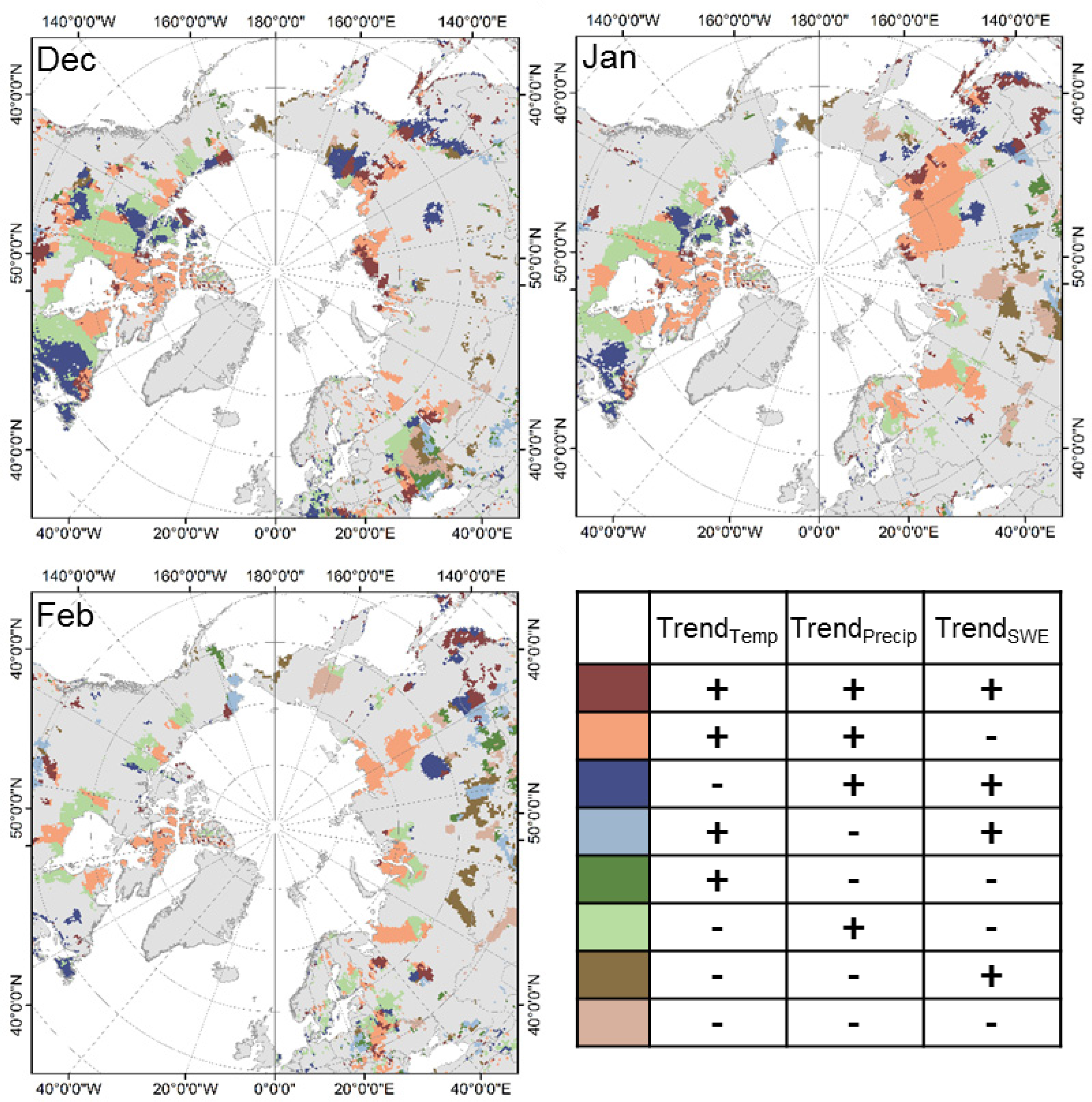
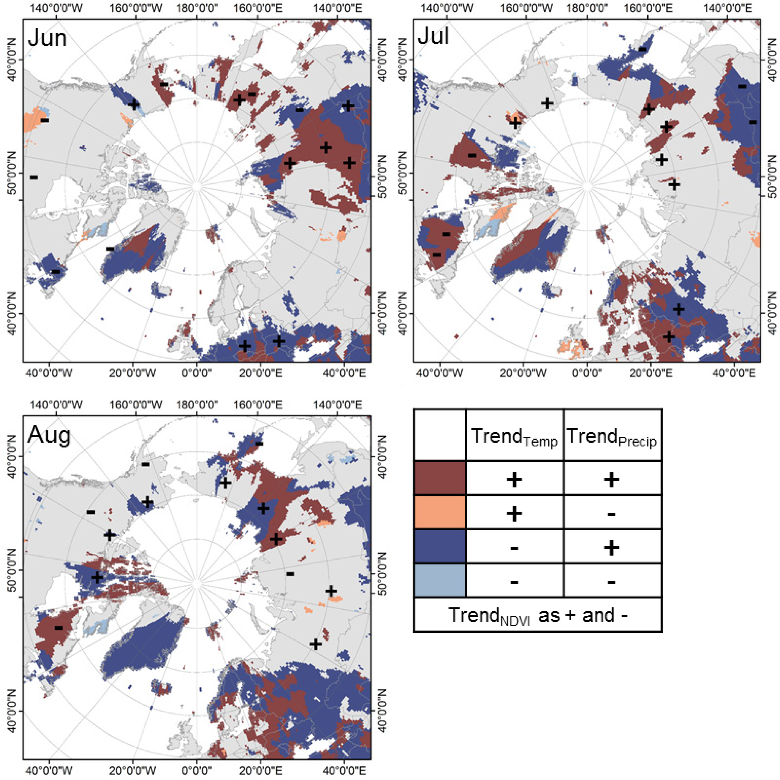
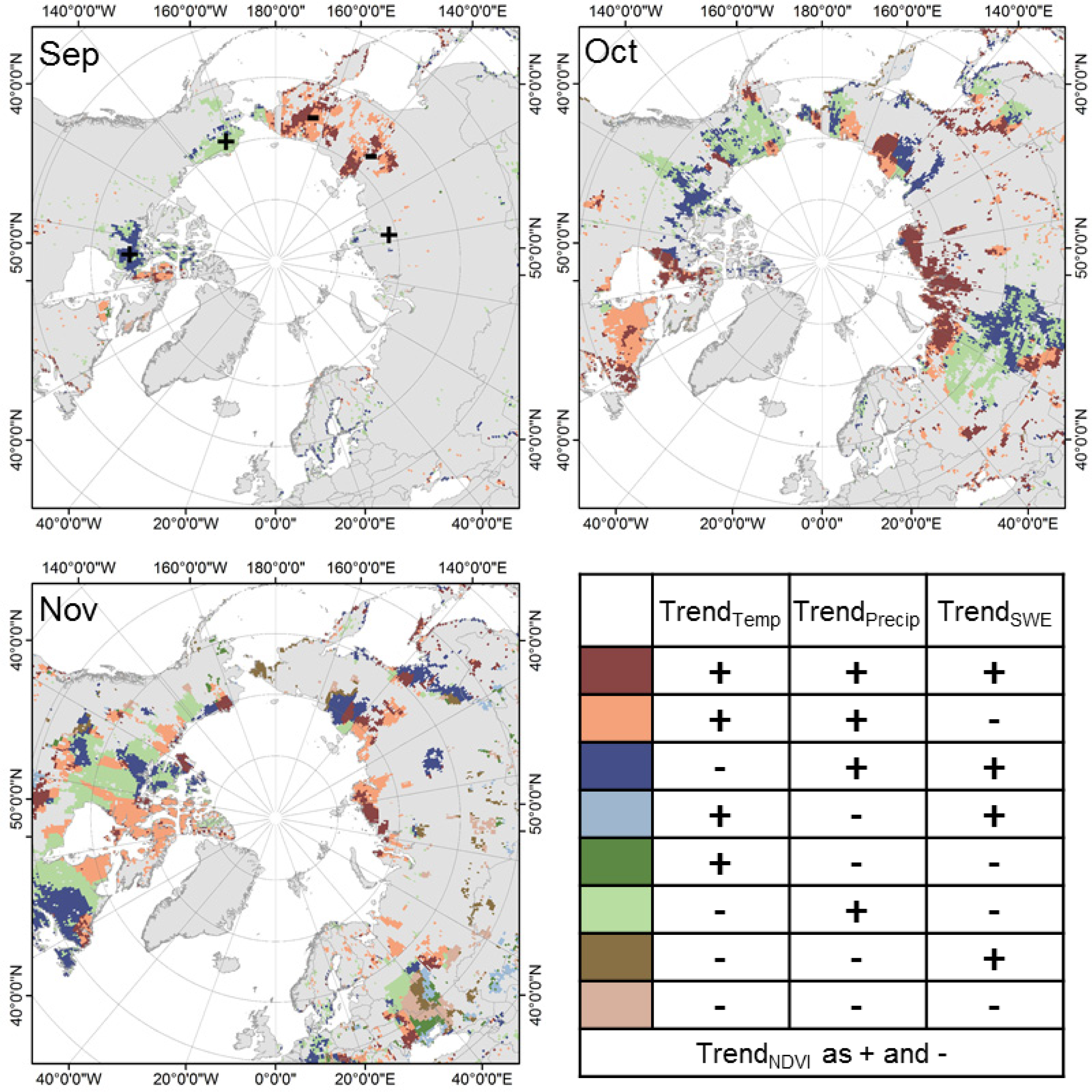
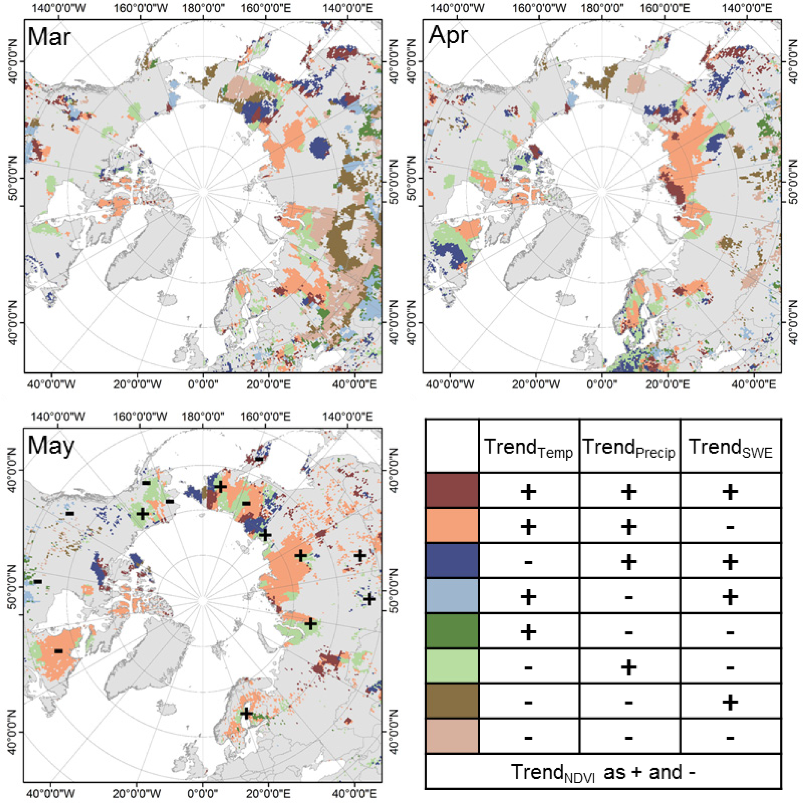
3.1. Pan-Arctic Trends on Monthly Scale

The co-occurrence analysis of different climatic and ecosystem parameters suggests the multi-scale feedbacks in the arctic ecosystems (Figures 1 and 4). The monthly trends were split into positive and negative values. The combination of different trend patterns from different parameters allows identifying regions having congruent and/or divergent trends when separating between positive and negative.
The winter months (Figure 1) are dominated by areas showing positive trends in temperature and precipitation in addition to negative SWEmax trends. The majority (approx. 40%) of the identified areas are characterized by this trend combination during the time of November to January. The second largest combination during the winter season is characterized by negative temperature and SWEmax and positive precipitation trends. However, the increasing precipitation trends are rather low in comparison to the other parameters. Approximately 20% of the significant trend regions are labeled by this type of trend combination.
The proportions of the trend findings remain the same until the end of March, as the area of the major trend combinations increasing towards the end of the winter season. The months of seasonal transition (April and May—Figure 2) are dominated by areas showing a decrease in SWEmax. This phenomenon can be referred to the early ablation of the snow cover, which also causes the early onset of the vegetation-growing period in these regions [10,14,72,73]. As the positive precipitation trends have their maxima during the summer months and very low trends in the other seasons, decreasing SWEmax trends are feasible at the end of the winter season.
During the summer months (Figure 3), regions with positive precipitation trends are covering the largest parts of the pan-arctic study area [74,75]. The area covered by positive and negative temperature trends is evenly distributed. As expected, no SWE information is available during the summer months June, July, and August. Hence, only temperature, precipitation and the NDVI trends are calculated and therefore displayed in a separate legend. During the months covering all four parameters, areas of negative SWEmax and positive temperature trends show an increase in NDVI, especially at the beginning and end of the growing season, which is an indicator for an early onset of the vegetation-growing season [76,77].
At the end of the growing season in September, only few significant trend regions can be identified, which are locally concentrated at the northernmost parts of the pan-arctic region (Figure 4). In October, half of the identified trend areas are characterized by rising precipitations and positive SWEmax areas are dominant. These trend regions are situated in the northern parts of the high latitudes. Further south, areas showing an opposite trend can be found [78].
The increase in early winter temperatures is changing the properties of the snow pack as well as the snow structure. Late fall (Figure 4) and early winter are very dynamic, with alternating rain and snow events. This is reducing the snow accumulation at the start of the winter season [43]. Hence, the SWEmax is reduced over time and results in a negative trend. Towards the end of the winter season (Figure 2), the negative SWEmax trend areas are increasing in size caused by an earlier and faster snow melt in the late winter months [43,78,79], accompanied by positive temperature trends. Moreover, the properties of the snowpack are influenced by changes in the frequencies of snow melt during the transition seasons, rain as well as the development of an ice layer on top of the snow pack [79].
In Siberia, multiple trend combinations are found compared to other regions on pan-arctic scale. Especially in March, the southern parts are dominated by various multivariate trend patterns. During the winter season, Siberia is dominated by an increase in precipitation and temperature, which is accompanied by decreasing SWEmax trends. However, the precipitation trends are fairly low compared to the temperature trends. During the summer, larger trend areas are found compared to other regions. In September, at the end of the growing season, no significant trend areas are visible. The NDVI trends are concentrated around the northernmost parts of Siberia. Especially, the Taymyr and Yamal Peninsula show a significant increase in the NDVI signal [72].
In difference to Siberia, the trends around the Bering Strait are dominated by negative precipitation with both positive and negative temperature trends, with all areas showing a negative trend in SWEmax. This region is dominated by ocean circulation coming from the northern pacific, the Chukchi Sea as well as the continental territories of Siberia [80]. The most significant trends are found for the transition times after the winter and the summer season. During the summer months, only few significant trend areas are found. Nevertheless, the majority of the area is dominated by increasing trends in all observed parameters. In contrast to all other regions, the Bering Strait shows significant trend areas in September. This month is dominated by increasing precipitation. The North Slope shows some trend patterns during the transition times between the seasons, which have been also described in [79]. The Hudson Bay region is showing the same but smaller area trend patterns than the Siberian territories [81].

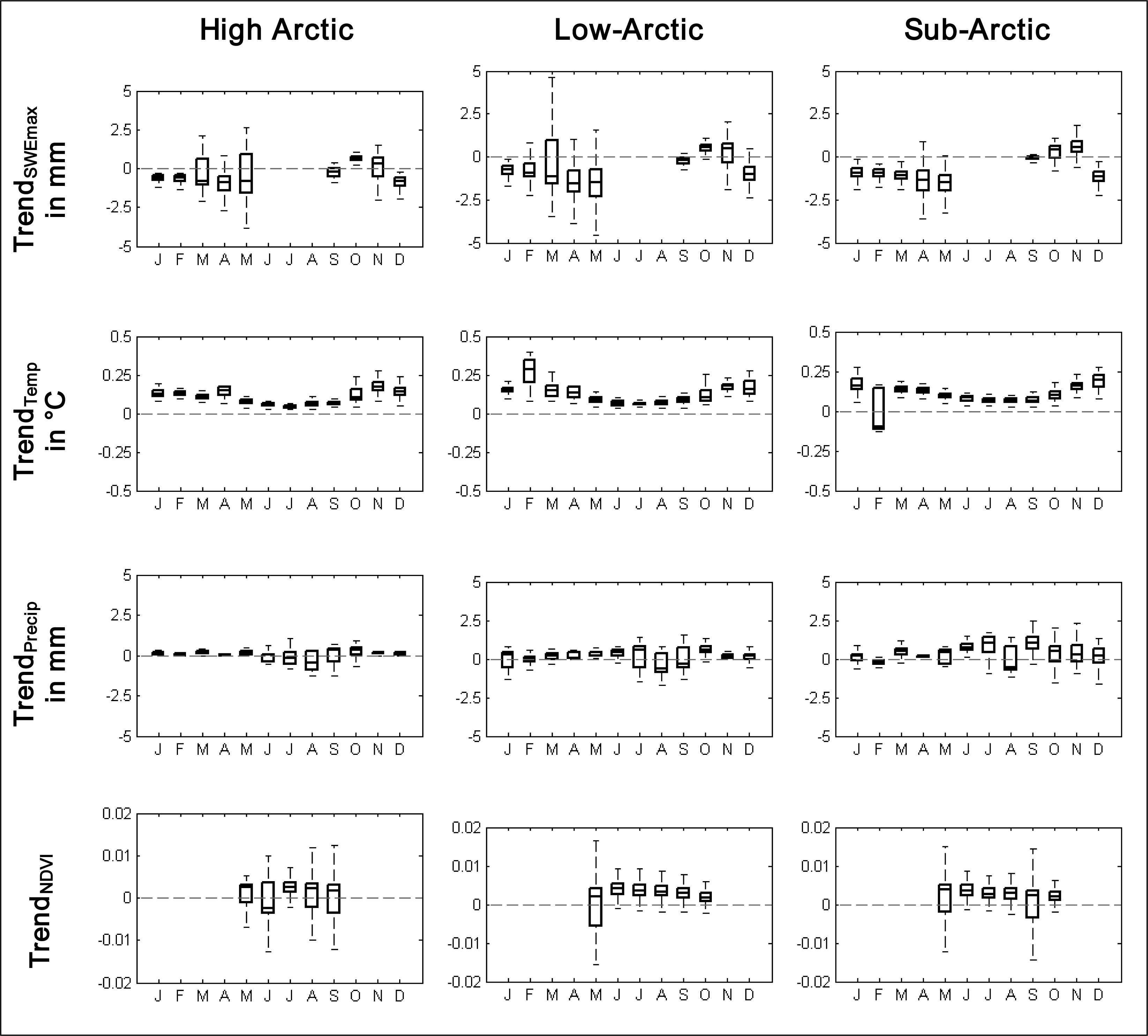
3.2. Monthly Inter-Annual Trend Dynamics for Different Arctic Regions

Trend findings have been analyzed for three regions, dividing the pan-arctic regions in high-arctic, the low-arctic, as well as the sub-arctic, according to the CAFF (Conservation of Arctic Flora and Fauna) definition (shown in the supplementary material Figure S1). For each parameter the yearly trend dynamics are shown in Figure 5. The individual boxplots are showing a monthly summary of the pixel values of each sub region. In comparison to the spatial analysis, the strength, the magnitude, and the dynamics of the trends are displayed.
The SWEmax trends are showing high dynamics in March for high and low-arctic regions. In general, variability is increasing while the majority of the SWEmax trends are decreasing towards the snow free period. The low-arctic (the median Ø−1.52 mm/year) and sub-arctic (Ø−1.43 mm/year) regions are characterized by the largest decline in SWEmax trend for April and May. For the time period from January to May, the largest magnitudes of trend findings are found for the low-arctic, indicating these regions to be highly dynamic during the last few decades [82,83]. Low positive SWEmax trends are found at the beginning of the winter season. In September, the high and low-arctic regions are showing a decrease in SWEmax (−0.23 mm/year and −0.21 mm/year), which is two times lower than for the sub-arctic regions (−0.12 mm/year). October and November are characterized by positive values (Ø 0.5 mm/year), whereas the majority of the regions during January to March are showing a decline in the SWEmax values (Ø−0.95 mm/year). The decrease in these snow cover properties will have a direct influence on extreme weather events, as well as the polar jet stream [84].
The intra-annual variability of the temperature trends follows a yearly cycle, which is similar for all three regions. In detail, the trend patterns are indicating that the winter season is dominated by larger positive temperature trends in comparison to the summer months. These findings have been also identified by [42]. This is especially true for the high-arctic and low-arctic regions. Compared to Figure 1 and 4, some parts of the sub-arctic regions are indicating a decline in winter temperatures, which is conform to the analysis of [85]. Comparing the summer and winter temperature trends, the majority of the winter trends (Ø 0.13 °C/year) are nearly twice as high as during the summer season (Ø 0.07 °C/year). The sub-arctic regions are showing a high magnitude in February, indicating declining temperature conditions (−0.10 °C/year). The same month is showing the highest temperature increase in the low-arctic region (0.28 °C/year). In general, the magnitudes of monthly temperature trends during the winter-time are showing the largest variations. The higher temperatures during the cold seasons and in the fall have a direct influence on the dynamics of the SWEmax in mid-winter season as well as the snow-melt in late winter [43,78,79]. Moreover, an increase in winter temperatures was identified to have a large impact on the vegetation structure, as damages maybe caused by the increase of these warming events [86].
In comparison to the other parameters, the precipitation trends are rather low. The median values from all months in all three regions range from −0.63 mm/year to 1.03 mm/year. However, the highest dynamics are found for the sub-arctic regions. The other regions have indicated similar trend patterns. From January to May, very low precipitation trends are found for the high-arctic (Ø 0.08 mm/year) and low-arctic regions (Ø 0.12 mm/year). The median values for the sub-arctic regions are twice as high during the same time period and also show higher dynamics. The largest precipitation trend variability are found in the summer and fall seasons. Especially the sub-arctic regions are showing the highest variability. During the summer season, the high arctic region is characterized by declining precipitation trends. During the fall and the beginning of the winter season, the sub-arctic regions are showing a higher increase in precipitation with a higher range of values when compared to the other parameters.
The monthly inter-annual dynamics of the NDVI trends are rather constant for the low and sub-arctic regions. Larger variability has been found for the high arctic regions. Nevertheless, the high-arctic region is characterized by relatively low vegetation cover. The focus should be more on the dynamics of the other land cover classes, including the taiga-tundra boundary as well as the boreal forest classes. In the perspective of climate change, these regions are of higher interest, as the appearing changes have a larger feedback to the climate system. For the low and sub-arctic higher NDVI trends at the beginning of the growing season are found. This might be an indicator of a shift in the onset of the vegetation-growing period in May, as observed in [87]. Towards the end of the summer season all regions are showing a decline in positive NDVI trends. Whereas the majority of NDVI trends are still positive for the low and sub-arctic, the high arctic indicates decreasing NDVI trends in October. In addition, a positive median, the sub-arctic regions are also showing negative NDVI trends in September, which might be referred to the boreal browning, found for some regions on pan-arctic scale [62]. Nevertheless, the transition time between the summer and winter months is dominated by areas with increasing NDVI trends. This phenomenon is connected to the enlargement of the vegetation active period in the arctic [77].

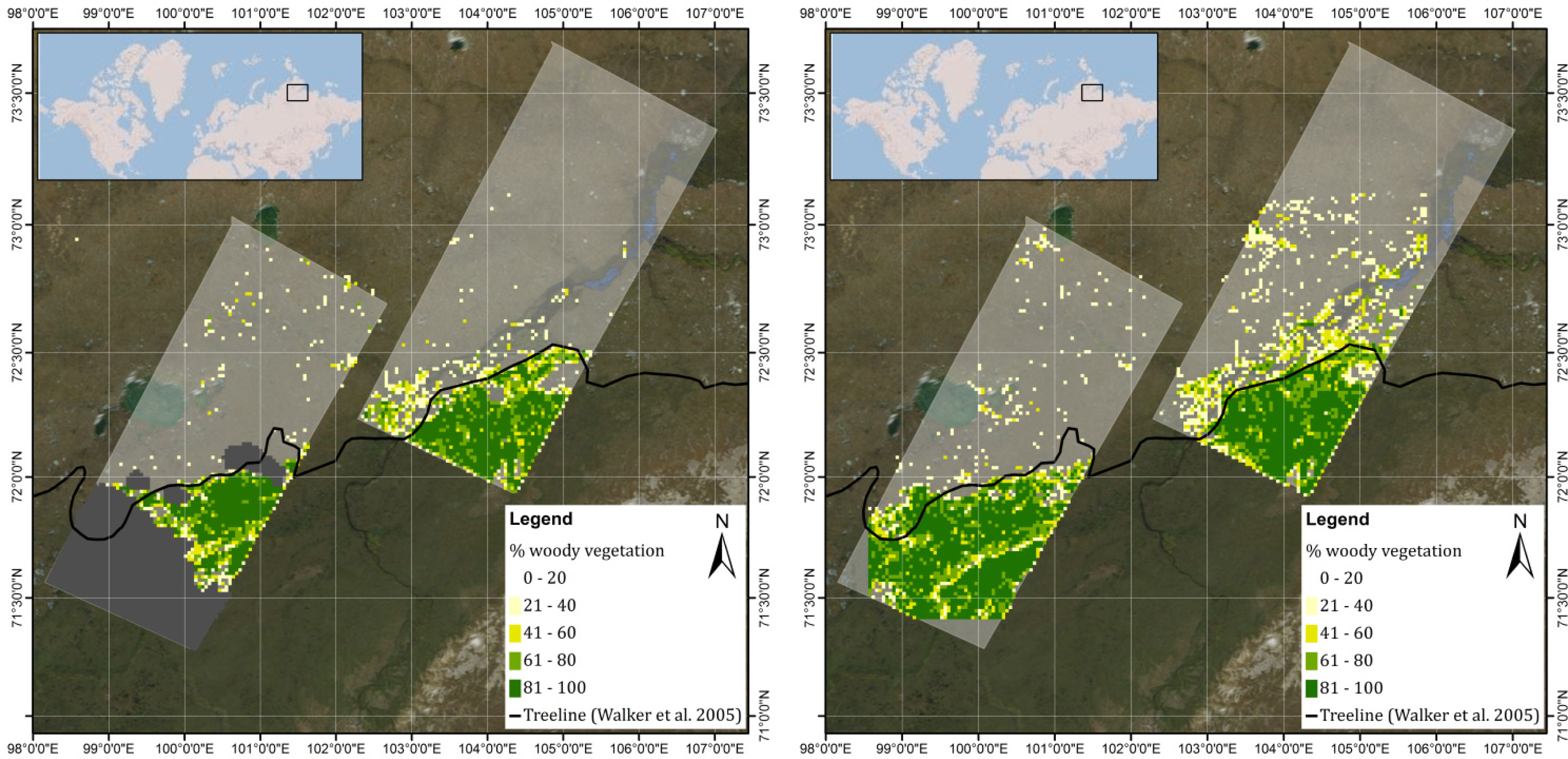
3.3. High-Resolution Change Mapping of the Taiga-Tundra Transition Zone in Northern Siberia

The Taymyr peninsula has been found to be one of the regions on pan-arctic scale showing the largest trends in different climate parameters during the last decades (Section 3.1). The trend analysis results from the previous section have shown the transition seasons to be characterized by positive temperature trends with a decline in maximum snow water equivalent for the area of the Taymyr peninsula. Daily air temperature (Tair) information from meteorological stations in this region are showing an increase during the last 40 years by approximately 3 °C (Figures 6 and S2), with an intensification of peak temperature events during the summer months [88,89].
Based on these observations, changes in woody vegetation cover have been analyzed by using historical and recent earth observation data. Figure 7 shows the changes of woody vegetation cover between 1973 and 2012. The majority of the cells situated south of the tree line reference, show woody vegetation cover values of greater than 60% for both time steps. The classification result of both time steps highly agrees with the separation of tundra from forested areas defined by the tree line reference from [58]. Unfortunately, the Landsat MSS mosaic is partly covered by clouds in the south. Both RapidEye images were free of clouds and ice.
When observing the transition zone between taiga and tundra, a decrease of woody vegetation cover percentage towards the northern parts becomes visible. The abrupt change at this vegetation border seems to be stronger in 1973, whereas, the recent years are characterized by a smoother transition. North of the tree line, only single patches of woody vegetation cover are detected. The patches are increasing in size, diameter and distribution in the recent years. Comparing both time steps, an increase in woody vegetation cover between 1973 and 2012 is obvious. Particularly, the fluvial terraces of the Khatanga river system are characterized by a higher amount of woody vegetation cover percentage in the RapidEye scenes.
The appearance of contiguous patches of woody vegetation north of the tree line is indicating a substantial impact to the ecosystem. This phenomenon is stronger in the eastern region in 2012, as this RapidEye scene is also from the same month as the Landsat MSS data. The western RapidEye scene is from September. Here the increase of woody vegetation patches is not significant, which might be due to the different observation time. When comparing July and September, the vegetation activity is already reduced towards the end of the growing season, which is influencing the ability to detect changes in the classification results.
Land cover classification and monitoring in the arctic regions using remote sensing information is a challenging issue due to snow, ice, and cloud cover, as well as the length of growing season [7]. Temporal variations between different acquisition times within the year need to be minimized when mapping land cover changes over long time periods [7]. In this study the acquisition times of the high resolution remote sensing data was July, except for one RapidEye scene, which was acquired in September. Hence, we expect the comparison of the western image pair to be affected by uncertainties due to the different acquisition months. Assessing the accuracy of the individual classification results was not possible, as information from in situ measurements is marginally available for the arctic regions. However, tree line change analysis using different data sources have been carried out for a small region in Ary-Mas (360 km2), indicating an encroachment of larch trees into the tundra region between 1973 and 2000 [33], which increases the confidence of the findings presented in this paper.

4. Conclusion

Multi-scale trends in the arctic ecosystems have been observed by analyzing the co-occurrence of climatic and ecosystem changes. The investigation of different spatial and temporal scales has highlighted multiple indicators of land cover changes related to climate-induced trends over the last decades. The highest temperature trends, twice as high as during the summer month, have been found during the winter season. Precipitation trends are rather low compared to the other parameters during the entire year, but considerably higher in summer and fall. The results from SWEmax and NDVI analysis have shown substantial modifications during the transition seasons of the year, potentially inducing and reflecting vegetation phenology shifts, resulting in longer vegetation periods and early spring green up. Particularly the low-arctic region, representing the taiga-tundra boundary, has the highest trends in all observed parameters. On a local scale, high-resolution land cover change analysis has shown increasing woody vegetation cover towards the northernmost regions dominated by tundra vegetation indicating a northwards shift of the tree line in a site of Taymyr Peninsula.
The consistent and operational monitoring of different essential climate and ecosystem parameters is of high importance for future arctic research. Earth observation data and techniques from various sources are available to retrieve spatial information and compensate the lack of ground measurements for remote areas. As the coverage of available meteorological stations in the arctic is sparse, the interpolation between the climate stations is introducing uncertainties of unknown magnitude, which needs to be taken into account. Hence, the continuity of satellite observation services for the integration of long-term time series information into climate monitoring and modeling approaches is essential. The synergetic combination of different information sources has shown the potential of identifying the co-occurrence of various climate parameters. Future studies should focus on the integration of data sources from different spatial and temporal scales. Additionally, the assessment of uncertainties and error sources is an essential issue for the investigation of remote sensing products. The identification of trend hot spot regions can create the basis (in terms of detecting regions of above average environmental change) for using observation data with higher spatial resolution. In combination with available ground measurements, the above-shown multi-scale approaches contribute to an increased confidence of land change magnitudes and ensure a high potential for future climate change and land monitoring research in the arctic.

Supplementary Information

remotesensing-06-02296-s001.pdf

Acknowledgments

The authors would like to thank the entire GIMMS group for permitting the usage of the NDVI3g dataset. We thank the team of Climate Research Unit for the provision of the temperature and precipitation data. Additional acknowledgements are given to the GlobSnow group of the Finnish Meteorological Institute for producing and providing the snow water equivalent information. Finally, the authors would like to thank the team of the RapidEye Science Archive of the German Aerospace Center for the provision of the RapidEye images (RESA Project ID: 473).

Author Contribution

Marcel Urban wrote the manuscript and was responsible for the research design, data preparation and analysis. Matthias Forkel and Jonas Eberle provided some of the data and gave relevant technical support. Christian Hüttich supported the analysis and interpretation of the results. Christiane Schmullius and Martin Herold provided significant input to the research design. All of the authors contributed in editing and reviewing the manuscript.

Conflicts of Interest

The authors declare no conflict of interest

References and Notes

  1. Moritz, R.E.; Bitz, C.M.; Steig, E.J. Dynamics of recent climate change in the Arctic. Science 2002, 297, 1497–1502. [Google Scholar]
  2. Grace, J.; Beringer, F.; Laszlo, N. Impacts of climate change on the tree line. Ann. Bot 2002, 90, 537–544. [Google Scholar]
  3. Nelson, F.E. (Un)frozen in Time. Science 2003, 69, 8–10. [Google Scholar]
  4. Miller, G.H.; Brigham-Grette, J.; Alley, R.B.; Anderson, L.; Bauch, H.A.; Douglas, M.S.V.; Edwards, M.E.; Elias, S.A.; Finney, B.P.; Fitzpatrick, J.J.; et al. Temperature and precipitation history of the Arctic. Quat. Sci. Rev 2010, 29, 1679–1715. [Google Scholar]
  5. Kaplan, J.O.; New, M. Arctic climate change with a 2 °C global warming: Timing, climate patterns and vegetation change. Clim. Chang 2006, 79, 213–241. [Google Scholar]
  6. Post, E.; Christensen, T.R.; Elberling, B.; Fox, A.D.; Gilg, O.; Forchhammer, M.C.; Bret-Harte, M.S.; Callaghan, T.V.; Hik, D.S.; Høye, T.T.; et al. Ecological dynamics across the Arctic associated with recent climate change. Science 2009, 325, 1355–1358. [Google Scholar]
  7. Stow, D.A.; Hope, A.; McGuire, D.; Verbyla, D.; Gamon, J.; Huemmrich, F.; Houston, S.; Racine, C.; Sturm, M.; Tape, K.; et al. Remote sensing of vegetation and land-cover change in Arctic Tundra Ecosystems. Remote Sens. Environ 2004, 89, 281–308. [Google Scholar]
  8. Myneni, R.B.; Keeling, C.D.; Tucker, C.J.; Asrar, G.; Nemani, R.R. Increased plant growth in the northern high latitudes from 1981 to 1991. Nature 1997, 386, 698–702. [Google Scholar]
  9. Romanovsky, V.; Burgess, M.; Smith, S.; Yoshikawa, K.; Brown, J. Permafrost temperature records: Indicators of climate change. EOS Trans. AGU 2002, 83, 589–594. [Google Scholar]
  10. Serreze, M.C.; Walsh, J.E.; Osterkamp, T.E.; Dyurgerov, M.; Romanovsky, V.E.; Oechel, W.C.; Morison, J.; Zhang, T.; Barry, R.G. Observational evidence of recent change in the northern high-latitude environment. Clim. Chang 2000, 46, 159–207. [Google Scholar]
  11. Overpeck, J.; Hughen, K.; Hardy, D.; Bradley, R.; Case, R.; Douglas, M.; Finney, B.; Gajewski, K.; Jacoby, G.; Jennings, A.; et al. Arctic environmental change of the last four centuries. Science 1997, 278, 1251–1256. [Google Scholar]
  12. Crowley, T.J. Causes of climate change over the past 1000 years. Science 2000, 289, 270–277. [Google Scholar]
  13. Chapin, F.S., III; Sturm, M.; Serreze, M.C.; McFadden, J.P.; Key, J.R.; Lloyd, A.H.; McGuire, A.D.; Rupp, T.S.; Lynch, A.H.; Schimel, J.P.; et al. Role of land-surface changes in arctic summer warming. Science 2005, 310, 657–660. [Google Scholar]
  14. Loranty, M.M.; Goetz, S.J.; Beck, P.S.A. Tundra vegetation effects on pan-Arctic albedo. Environ. Res. Lett 2011, 6, 1–7. [Google Scholar]
  15. Blok, D.; Sass-Klaassen, U.; Schaepman-Strub, G.; Heijmans, M.M.P.D.; Sauren, P.; Berendse, F. What are the main climate drivers for shrub growth in Northeastern Siberian tundra? Biogeosciences 2011, 8, 1169–1179. [Google Scholar] [Green Version]
  16. Xu, L.; Myneni, R.B.; Chapin, F.S., III; Callaghan, T.V.; Pinzon, J.E.; Tucker, C.J.; Zhu, Z.; Bi, J.; Ciais, P.; Tømmervik, H.; et al. Temperature and vegetation seasonality diminishment over northern lands. Nat. Clim. Chang 2013, 3, 581–586. [Google Scholar]
  17. Beringer, J.; Tapper, N.J.; Mchugh, I.; Chapin, F.S., III; Lynch, A.H.; Serreze, M.C.; Slater, A. Impact of Arctic treeline on synoptic climate. Geophys. Res. Lett 2001, 28, 4247–4250. [Google Scholar]
  18. Lawrence, D.M.; Slater, A.G.; Tomas, R.A.; Holland, M.M.; Deser, C. Accelerated Arctic land warming and permafrost degradation during rapid sea ice loss. Geophys. Res. Lett 2008, 35, 1–6. [Google Scholar]
  19. Bhatt, U.S.; Walker, D.A.; Raynolds, M.K.; Bieniek, P.A.; Epstein, H.E.; Comiso, J.C.; Pinzon, J.E.; Tucker, C.J; Polyakov, I.V. Recent declines in warming and vegetation greening trends over Pan-Arctic Tundra. Remote Sens 2013, 5, 4229–4254. [Google Scholar]
  20. Bokhorst, S.; Bjerke, J.W.; Bowles, F.W.; Melillo, J.; Callaghan, T.V.; Phoenix, G.K. Impacts of extreme winter warming in the sub-Arctic: Growing season responses of dwarf shrub heathland. Glob. Chang. Biol 2008, 14, 2603–2612. [Google Scholar]
  21. Myers-Smith, I.H.; Forbes, B.C.; Wilmking, M.; Hallinger, M.; Lantz, T.; Blok, D.; Tape, K.D.; Macias-Fauria, M.; Sass-Klaassen, U.; Lévesque, E.; et al. Shrub expansion in tundra ecosystems: Dynamics, impacts and research priorities. Environ. Res. Lett 2011, 6, 1–15. [Google Scholar]
  22. Blok, D.; Heijmans, M.M.P.D.; Schaepman-Strub, G.; Kononov, A.V.; Maximov, T.C.; Berendse, F. Shrub expansion may reduce summer permafrost thaw in Siberian tundra. Glob. Chang. Biol 2010, 16, 1296–1305. [Google Scholar]
  23. Tape, K.; Sturm, M.; Racine, C. The evidence for shrub expansion in Northern Alaska and the Pan-Arctic. Glob. Chang. Biol 2006, 12, 686–702. [Google Scholar]
  24. Berner, L.T.; Beck, P.S.A; Bunn, A.G.; Goetz, S.J. Plant response to climate change along the forest-tundra ecotone in northeastern Siberia. Glob. Chang. Biol 2013, 19, 3449–3462. [Google Scholar]
  25. Epstein, H.E.; Beringer, J.; Gould, W.A.; Lloyd, A.H.; Thompson, C.D.; Chapin, F.S., III; Michaelson, G.J.; Ping, C.L.; Rupp, T.S.; Walker, D.A. The nature of spatial transitions in the Arctic. J. Biogeogr 2004, 31, 1917–1933. [Google Scholar]
  26. Sturm, M.; Racine, C.H.; Tape, K.D.; Cronin, T.W.; Caldwell, R.L.; Marshall, J. Increasing shrub abundance in the Arctic. Nature 2001, 411, 546–547. [Google Scholar]
  27. Bunn, A.G.; Goetz, S.J. Trends in satellite-observed circumpolar photosynthetic activity from 1982 to 2003: The influence of seasonality, cover type, and vegetation density. Earth Interact 2006, 10, 1–19. [Google Scholar]
  28. Ranson, K.J.; Sun, G.; Kharuk, V.I.; Kovacs, K. Assessing tundra–taiga boundary with multi-sensor satellite data. Remote Sens. Environ 2004, 93, 283–295. [Google Scholar]
  29. Shiyatov, S.G. Rates of change in the upper treeline ecotone in the Polar Ural Mountains. Pages News 2003, 11, 8–10. [Google Scholar]
  30. Harsch, M.A.; Hulme, P.P.; McGlone, M.S.; Duncan, R.P. Are treelines advancing? A global meta-analysis of treeline response to climate warming. Ecol. Lett 2009, 12, 1040–1049. [Google Scholar]
  31. Olthof, I.; Pouliot, D. Treeline vegetation composition and change in Canada’s western Subarctic from AVHRR and canopy reflectance modeling. Remote Sens. Environ 2010, 114, 805–815. [Google Scholar]
  32. Sun, G.; Ranson, K.; Kharuk, V. Characterization and Monitoring of Tundra-Taiga Transition Zone with Multi-Sensor Satellite Data. In Eurasian Arctic Land Cover and Land Use in a Changing Climate; Gutman, G., Reissell, A., Eds.; Springer: Dordrecht, The Netherlands, 2011; pp. 53–77. [Google Scholar]
  33. Kharuk, V.I.; Ranson, K.J.; Im, S.T.; Naurzbaev, M.M. Forest-tundra larch forests and climatic trends. Russ. J. Ecol 2006, 37, 291–298. [Google Scholar]
  34. CAFF. Arctic Biodiversity Trends 2010 Selected Indicators of Change, 1st ed; Kurvits, T., Alfthan, B., Mork, E., Eds.; Conservation of Arctic Flora and Fauna: Akureyri, Iceland, 2010. [Google Scholar]
  35. Luojus, K.; Pulliainen, J.; Takala, M.; Lemmetyinen, J.; Kangwa, M.; Solberg, R.; Rott, H.; Derksen, C.; Wiesmann, A.; Metsämäki, S.; et al. Global Snow Monitoring for Climate Research Final Report, 2011. World Meteorological Organization. Available online: http://www.wmo.int/pages/prog/www/OSY/Meetings/GCW-IM1/Doc11.1_GlobSnow_Report.pdf (accessed on 1 March 2014).
  36. Pulliainen, J. Mapping of snow water equivalent and snow depth in boreal and sub-arctic zones by assimilating space-borne microwave radiometer data and ground-based observations. Remote Sens. Environ 2006, 101, 257–269. [Google Scholar]
  37. Takala, M.; Luojus, K.; Pulliainen, J.; Derksen, C.; Lemmetyinen, J.; Kärnä, J.-P.; Koskinen, J.; Bojkov, B. Estimating northern hemisphere snow water equivalent for climate research through assimilation of space-borne radiometer data and ground-based measurements. Remote Sens. Environ 2011, 115, 3517–3529. [Google Scholar]
  38. Hancock, S.; Baxter, R.; Evans, J.; Huntley, B. Evaluating global snow water equivalent products for testing land surface models. Remote Sens. Environ 2013, 128, 107–117. [Google Scholar] [Green Version]
  39. Jones, P.D.; Moberg, A. Hemispheric and large-scale surface air temperature variations: An extensive revision and an update to 2001. J. Clim 2003, 16, 206–223. [Google Scholar]
  40. New, M.; Hulme, M.; Jones, P. Representing twentieth-century space-time climate variability. Part II: Development of 1901–96 monthly grids of terrestrial surface climate. J. Clim 2000, 2217–2238. [Google Scholar]
  41. New, M.; Hulme, M.; Jones, P. Representing twentieth-century space-time climate variability. Part I: Development of a 1961–90 mean monthly terrestrial climatology. J. Clim 1999, 12, 829–856. [Google Scholar]
  42. Semenov, V.A.; Latif, M. The early twentieth century warming and winter Arctic sea ice. Cryosphere Discuss 2012, 6, 2037–2057. [Google Scholar]
  43. Brown, R.; Derksen, C.; Wang, L. A multi-data set analysis of variability and change in Arctic spring snow cover extent, 1967–2008. J. Geophys. Res 2010, 115, 1–16. [Google Scholar]
  44. Park, H.; Walsh, J.E.; Kim, Y.; Nakai, T.; Ohata, T. The role of declining Arctic sea ice in recent decreasing terrestrial Arctic snow depths. Polar Sci 2013, 7, 174–187. [Google Scholar]
  45. Rawlins, M.A.; Willmott, C.J.; Shiklomanov, A.; Linder, E.; Frolking, S.; Lammers, R.B.; Vörösmarty, C.J. Evaluation of trends in derived snowfall and rainfall across Eurasia and linkages with discharge to the Arctic Ocean. Geophys. Res. Lett 2006, 33, 1–4. [Google Scholar]
  46. Tucker, C.J.; Pinzon, J.E.; Brown, M.E.; Slayback, D.A.; Pak, E.W.; Mahoney, R.; Vermote, E.F.; El Saleous, N. An extended AVHRR 8-km NDVI dataset compatible with MODIS and SPOT vegetation NDVI data. Int. J. Remote Sens 2005, 26, 4485–4498. [Google Scholar]
  47. Slayback, D.A.; Pinzon, J.E.; Los, S.O.; Tucker, C.J. Northern hemisphere photosynthetic trends 1982–99. Glob. Chang. Biol 2003, 9, 1–15. [Google Scholar]
  48. Epstein, H.E.; Raynolds, M.K.; Walker, D.A.; Bhatt, U.S.; Tucker, C.J.; Pinzon, J.E. Dynamics of aboveground phytomass of the circumpolar Arctic tundra during the past three decades. Environ. Res. Lett 2012, 7, 1–12. [Google Scholar]
  49. Piao, S.; Wang, X.; Ciais, P.; Zhu, B.; Wang, T.; Liu, J. Changes in satellite-derived vegetation growth trend in temperate and boreal Eurasia from 1982 to 2006. Glob. Chang. Biol 2011, 17, 3228–3239. [Google Scholar]
  50. Macias-Fauria, M.; Forbes, B.C.; Zetterberg, P.; Kumplala, T. Eurasian Arctic greening reveals teleconnections and the potential for structurally novel ecosystems. Nat. Clim. Chang 2012, 2, 613–618. [Google Scholar] [Green Version]
  51. Wang, X.; Piao, S.; Ciais, P.; Li, J.; Friedlingstein, P.; Koven, C.; Chen, A. Spring temperature change and its implication in the change of vegetation growth in North America from 1982 to 2006. Proc. Natl. Acad. Sci. USA 2011, 108, 1240–1245. [Google Scholar]
  52. Urban, M.; Forkel, M.; Schmullius, C.; Hese, S.; Hüttich, C.; Herold, M. Identification of land surface temperature and albedo trends in AVHRR Pathfinder data from 1982 to 2005 for northern Siberia. Int. J. Remote Sens 2013, 34, 4491–4507. [Google Scholar]
  53. Zhu, Z.; Bi, J.; Pan, Y.; Ganguly, S.; Anav, A.; Xu, L.; Samanta, A.; Piao, S.; Nemani, R.R.; Myneni, R. Global data sets of Vegetation Leaf Area Index (LAI)3g and fraction of Photosynthetically Active Radiation (FPAR)3g derived from Global Inventory Modeling and Mapping Studies (GIMMS) Normalized Difference Vegetation Index (NDVI3g) for the period 1981 to 2011. Remote Sens 2013, 5, 927–948. [Google Scholar]
  54. Gleason, A.C.R.; Prince, S.D.; Goetz, S.J.; Small, J. Effects of orbital drift on land surface temperature measured by AVHRR thermal sensors. Remote Sens. Environ 2002, 79, 147–165. [Google Scholar]
  55. Julien, Y.; Sobrino, J.A. Correcting AVHRR long term data record V3 estimated LST from orbital drift effects. Remote Sens. Environ 2012, 123, 207–219. [Google Scholar]
  56. Pinzon, J.E. Revisiting error, precision and uncertainty in NDVI AVHRR data: development of a consistent NDVI3g time series. Remote Sens 2013. submitted. [Google Scholar]
  57. Holben, B.N. Characteristics of maximum-value composite images from temporal AVHRR data. Int. J. Remote Sens 1986, 7, 1417–1434. [Google Scholar]
  58. Walker, A.D.; Raynolds, M.K.; Daniels, F.J.A.; Einarsson, E.; Elvebakk, A.; Gould, W.A.; Katenin, A.E.; Kholod, S.S.; Markon, C.J.; Melnikov, E.S.; et al. The circumpolar Arctic vegetation map. J. Veg. Sci 2005, 16, 267–282. [Google Scholar]
  59. Talbot, S.; Meades, W. Circumboreal Vegetation Map (CBVM) Mapping the Green Halo—Concept Paper; CAFF International Secretariat: Akureyri, Iceland, 2011. [Google Scholar]
  60. Goetz, S.J.; Bunn, A.G.; Fiske, G.J.; Houghton, R.A. Satellite-observed photosynthetic trends across boreal North America associated with climate and fire disturbance. Proc. Natl. Acad. Sci. USA 2005, 102, 13521–13525. [Google Scholar]
  61. De Jong, R.; de Bruin, S.; de Wit, A.; Schaepman, M.E.; Dent, D.L. Analysis of monotonic greening and browning trends from global NDVI time-series. Remote Sens. Environ 2011, 115, 692–702. [Google Scholar] [Green Version]
  62. Forkel, M.; Carvalhais, N.; Verbesselt, J.; Mahecha, M.D.; Neigh, C.S.R.; Reichstein, M. Trend change detection in NDVI time series: Effects of inter-annual variability and methodology. Remote Sens 2013, 5, 2113–2144. [Google Scholar]
  63. Mann, H.B. Nonparametric tests against trend. Econometrica 1945, 13, 245–259. [Google Scholar]
  64. Jacoby, G.C.; Lovelius, N.V.; Shumilov, O.I.; Raspopov, O.M.; Karbainov, J.M.; Frank, D.C. Long-term temperature trends and tree growth in the Taymir Region of Northern Siberia. Quat. Res 2000, 53, 312–318. [Google Scholar]
  65. Shvidenko, A.Z.; Gustafson, E.; Mcguire, A.D.; Kharuk, V.I.; Schepaschenko, D.G.; Shugart, H.H.; Tchebakova, N.M.; Vygodskaya, N.N.; Onuchin, A.A.; Hayes, D.J.; et al. Terrestrial Ecosystems and Their Change. In Regional Environmental Changes in Siberia and Their Global Consequences; Groisman, P.Y., Gutman, G., Eds.; Springer Netherlands: Dordrecht, The Netherlands, 2013; pp. 171–249. [Google Scholar]
  66. Kharuk, V.I.; Dvinskaya, M.L.; Ranson, K.J.; Im, S.T. Expansion of evergreen conifers to the larch-dominated zone and climatic trends. Russ. J. Ecol 2005, 36, 164–170. [Google Scholar]
  67. MacDonald, G.M.; Kremenetski, K.V.; Beilman, D.W. Climate change and the northern Russian treeline zone. Philos. Trans. R. Soc. B 2008, 363, 2283–2299. [Google Scholar]
  68. Sidorova, O.V.; Siegwolf, R.T.W.; Saurer, M.; Naurzbaev, M.M.; Shashkin, A.V.; Vaganov, E.A. Spatial patterns of climatic changes in the Eurasian north reflected in Siberian larch tree-ring parameters and stable isotopes. Glob. Chang. Biol 2010, 16, 1003–1018. [Google Scholar]
  69. Landsat: MSS Scene; LM11590081973207AAA05; NASA Landsat Programm: Sioux Falls, SD, USA, 1973.
  70. Landsat: MSS Scene; LM11590091973207AAA05; NASA Landsat Programm: Sioux Falls, SD, USA, 1973.
  71. Richter, R. A spatially adaptive fast atmospheric correction algorithm. Int. J. Remote Sens 1996, 17, 1201–1214. [Google Scholar]
  72. Eastman, J.R.; Sangermano, F.; Machado, E.A.; Rogan, J.; Anyamba, A. Global trends in seasonality of normalized difference vegetation index (NDVI), 1982–2011. Remote Sens 2013, 5, 4799–4818. [Google Scholar]
  73. Liston, G.E.; Hiemstra, C.A. The changing cryosphere: Pan-Arctic snow trends (1979–2009). J. Clim 2011, 24, 5691–5712. [Google Scholar]
  74. Kattsov, V.M.; Källén, E.; Cattle, H.; Christensen, J.; Drange, H.; Hanssen-bauer, I.; Jóhannesen, T.; Karol, I.; Räisänen, J.; Svensson, G.; et al. Future Climate Change: Modeling and Scenarios for the Arctic. In Arctic Climate Impact Assessment—Scientific Report; Symon, C., Arris, L., Heal, B., Eds.; Cambridge University Press: Cambridge, UK, 2005. [Google Scholar]
  75. Peili, W.; Haak, H.; Wood, R.; Jungclaus, J.; Furevik, T. Simulating the Terms in the Arctic Hydrological Budget. In Arctic-Subarctic Ocean Fluxes: Defining the Role of the Northern Seas in Climate; Dickson, R., Meincke, J., Rhines, P., Eds.; Springer: Dordrecht, The Netherlands, 2008; pp. 363–384. [Google Scholar]
  76. Hüttich, C.; Herold, M.; Schmullius, C.; Egorov, V.; Bartalev, S.A. Indicators of Northern Eurasia’s land-cover change trends from SPOT-VEGETATION time-series analysis 1998–2005. Int. J. Remote Sens 2007, 28, 4199–4206. [Google Scholar]
  77. Delbart, N.; Picard, G.; Le Toan, T.; Kergoat, L.; Quegan, S.; Woodward, I.; Dye, D.; Fedotova, V. Spring phenology in boreal Eurasia over a nearly century time scale. Glob. Chang. Biol 2008, 14, 603–614. [Google Scholar]
  78. Räisänen, J. Warmer climate: Less or more snow? Clim. Dyn 2007, 30, 307–319. [Google Scholar]
  79. Martin, P.D.; Jenkins, J.L.; Adams, F.J.; Jorgenson, M.T.; Matz, A.C.; Payer, D.C.; Reynolds, P.E.; Tidwell, A.C.; Zelenak, J.R. Wildlife Response to Environmental Arctic Change: Predicting Future Habitats of Arctic Alaska, 2009. U.S. Fish and Wildlife Service; p. 138. Available online: http://www.fws.gov/alaska/pdf/wildreach_workshop_report.pdf (accessed on 7 March 2014).
  80. Callaghan, T.V.; Johansson, M.; Brown, R.D.; Groisman, P.Y.; Labba, N.; Radionov, V.; Barry, R.G.; Bulygina, O.N.; Essery, R.L.H.; Frolov, D.M.; et al. The Changing Face of Arctic Snow Cover: A Synthesis of Observed and Projected Changes. AMBIO 2011, 40, 17–31. [Google Scholar]
  81. Gagnon, A.S.; Gough, W.A. Hydro-climatic trends in the Hudson Bay Region, Canada. Can. Water Resour. J 2002, 27, 245–262. [Google Scholar]
  82. Walker, D.A.; Jia, G.J.; Epstein, H.E.; Raynolds, M.K.; Chapin, F.S., III; Copass, C.; Hinzman, L.D.; Knudson, J.; Maier, H.; Michaelson, G.J.; et al. Vegetation-soil-thaw-depth relationships along a low-arctic bioclimate gradient, Alaska: Synthesis of information from the ATLAS studies. Permafr. Periglac. Process 2003, 14, 103–123. [Google Scholar]
  83. Comiso, J.C.; Parkinson, C.L.; Gersten, R.; Stock, L. Accelerated decline in the Arctic sea ice cover. Geophys. Res. Lett 2008, 35, 1–6. [Google Scholar]
  84. Francis, J.A.; Vavrus, S.J. Evidence linking Arctic amplification to extreme weather in mid-latitudes. Geophys. Res. Lett 2012, 39, 1–6. [Google Scholar]
  85. Cohen, J.L.; Furtado, J.C.; Barlow, M.; Alexeev, V.; Cherry, J.E. Arctic warming, increasing snow cover and widespread boreal winter cooling. Environ. Res. Lett 2012, 7, 1–8. [Google Scholar]
  86. Bokhorst, S.F.; Bjerke, J.W.; Tømmervik, H.; Callaghan, T.V.; Phoenix, G.K. Winter warming events damage sub-Arctic vegetation: consistent evidence from an experimental manipulation and a natural event. J. Ecol 2009, 97, 1408–1415. [Google Scholar]
  87. Picard, G.; Quegan, S.; Delbart, N.; Lomas, M.R.; Le Toan, T.; Woodward, F.I. Bud-burst modelling in Siberia and its impact on quantifying the carbon budget. Glob. Chang. Biol 2005, 11, 2164–2176. [Google Scholar]
  88. Global Surface Summary of the Day: GSOD 2012; National Climatic Data Center: Asheville, NC, USA, 2012.
  89. Eberle, J.; Clausnitzer, S.; Hüttich, C.; Schmullius, C. Multi-source data processing middleware for land monitoring within a web-based spatial data infrastructure for Siberia. ISPRS Int. J. Geo-Inf 2013, 2, 553–576. [Google Scholar]
Figure 1. Co-occurrence of different climatic and ecosystem trends on pan-arctic scale between 1981 and 2012 (December to February). The trend findings from monthly temperatures, precipitation, SWEmax are combined into one information source, which includes all possible combinations of trend patterns. Only areas showing significant trends (p-value < 0.05) are displayed.
Remotesensing 06 02296f1
Figure 2. Co-occurrence of different climatic and ecosystem trends on pan-arctic scale between 1981 and 2012 (March to May) (for more explanation see Figure 1). The NDVI is shown via plus or minus symbols, which are indicating either positive or negative trends at the location.
Remotesensing 06 02296f2
Figure 3. Co-occurrence of different climatic and ecosystem trends on pan-arctic scale between 1981 and 2012 (June to August). The trend findings from monthly temperatures and precipitation were combined into one information source. The NDVI is shown via plus or minus symbols, which are indicating either positive or negative trends at the location.
Remotesensing 06 02296f3
Figure 4. Co-occurrence of different climatic and ecosystem trends on pan-arctic scale between 1981 and 2012 (September to November) (for more explanation see Figure 1).
Remotesensing 06 02296f4
Figure 5. Monthly inter-annual variability of the slopes from the multivariate trend calculations. Only trends with a significance level of p < 0.05 are shown.
Remotesensing 06 02296f5
Figure 6. Air-Temperature time series divided by seasons (winter—DJF; spring—MAM, summer—JJA and fall—SON) of the meteorological station Khatanga at the Taymyr Peninsula (71.9°N, 102.5°E)—Additional stations are shown in the supplementary material (Figure S2).
Remotesensing 06 02296f6
Figure 7. Landsat MSS and RapidEye woody vegetation cover (in % per 5 km grid cell) mapping between 1973 (Left) and 2012 (Right)—background based on World Imagery by ESRI. The tree line reference from [58] is shown in black. Cloud regions in the Landsat MSS data are shown in grey.
Remotesensing 06 02296f7

