Separating Crop Species in Northeastern Ontario Using Hyperspectral Data

Abstract

The purpose of this study was to examine the capability of hyperspectral narrow wavebands within the 400–900 nm range for distinguishing five cash crops commonly grown in Northeastern Ontario, Canada. Data were collected from ten different fields in the West Nipissing agricultural zone (46°24′N lat., 80°07′W long.) and included two of each of the following crop types; soybean (Glycine max), canola (Brassica napus L.), wheat (Triticum spp.), oat (Avena sativa), and barley (Hordeum vulgare). Stepwise discriminant analysis was used to assess the spectral separability of the various crop types under two scenarios; Scenario 1 involved testing separability of crops based on number of days after planting and Scenario 2 involved testing crop separability at specific dates across the growing season. The results indicate that select hyperspectral bands in the visual and near infrared (NIR) regions (400–900 nm) can be used to effectively distinguish the five crop species under investigation. These bands, which were used in a variety of combinations include B465, B485, B495, B515, B525, B535, B545, B625, B645, B665, B675, B695, B705, B715, B725, B735, B745, B755, B765, B815, B825, B885, and B895. In addition, although species classification could be achieved at any point during the growing season, the optimal time for satellite image acquisition was determined to be in late July or approximately 75–79 days after planting with the optimal wavebands located in the red-edge, green, and NIR regions of the spectrum.

1. Introduction

According to the 2011 Canadian census of agriculture, farmland has decreased by 10.3% (or 23,643 farms) since the last census in 2006. The size of farm stands has also decreased by 4.1%, yet the average size of the farms in Canada has increased by 6.9%. Total government spending (federal and provincial) in support of the Agriculture and Agri-Food sector increased to $7.5 billion in 2011–2012, representing 26.7% of agriculture GDP. Government spending on research and development in Agriculture and Agri-Food Canada reached over $560 million in the 2011–2012 fiscal year. Every year, millions of dollars are spent conducting inventories of crops across the country [1].

Remote sensing is a cost-effective, non-destructive and highly efficient method for conducting agricultural research including the estimation of biophysical parameters such as leaf area index (LAI) and chlorophyll content [2,3], identification of weed species [4,5], crop separation and classification [6–8], and yield estimation [9]. In the last few decades, numerous studies have demonstrated that remote sensing, in particular, hyperspectral remote sensing, is a more desirable option for conducting agricultural research as it provides contiguous reflectance data allowing the ability to monitor slight changes in crops using multiple bands [10–12]. One important application of hyperspectral remote sensing in agriculture is the ability to distinguish various crop types. Hyperspectral remote sensing can be used to monitor crops in both small and large-scale operations through the use of handheld devices, airborne devices or satellite imagery. Accurate crop identification through satellite imagery would allow government organizations and researchers to complete nationwide crop inventory in a cost-effective and non-intrusive way.

Several studies have used hyperspectral data to manage agricultural crops, many of which have focused on crop separability [3,8,13]. The most common method for collecting hyperspectral data was through the use of handheld spectroradiometers [14–18], however, reflectance data were also simulated using spectral reflectance models [19] or collected via hyperspectral satellite imagery [20–22]. Typically, studies that used handheld devices were conducted in the visible (350–700 nm) and near-infrared (NIR) portions of the electromagnetic spectrum (EMS). A number of studies have focused on discriminating weed species [5,7], different strands or cultivars of the same crop such as wheat, rice and cotton [6,23,24] and finally different species of crop altogether [8,22,25].

To examine the relationship between different crop species and hyperspectral data for the purpose of classifying different crop types, a number of methods are commonly used. Although some researchers reduced data dimension first [3], many used discriminant analysis [4,13], principal components analysis [4,8,26] and other classification methods such as partial least square regression [6], neural networks [27–29], and image-based data [21,30] to classify crop species. Many studies have determined that the visible and NIR portions of the EMS are significant in agricultural research, especially for estimating crop biophysical parameters such as leaf area index and chlorophyll content, in particular, for crop discrimination [3,8,13,30,31]. The wavebands identified as significant vary by location and by crop type, however, importance is often placed on the red-edge, NIR portions of the visible spectrum for crop separation [8,32–34].

Although a number of studies have examined the relationship between spectral reflectance and various crop types for the purpose of classifying crops, those studies often only collect data at certain growth stages throughout the growing season. It is arguable that due to the rapid changes in plant structure in the later growth stages of the growing season, crop separability might be maximized. Therefore, the purpose of this study is to determine the separability of crop species using hyperspectral narrow wavebands for five crop species including soybean (Glycine max), canola (Brassica napus L.), wheat (Triticum spp.), oat (Avena sativa), and barley (Hordeum vulgare) across the Northern Ontario growing season. More specifically, the objectives of this research are to determine the optimal narrow wavebands for discrimination of crops using a handheld spectroradiometer and to determine the optimal time for crop separability by number of days after planting (DAP) and by specific dates across the growing season near Verner, Ontario (46.37°N, 79.93°W). The information derived from this study can then be used as a guide for determining what type of remote sensing data should be acquired at any particular time in the Northern Ontario growing season, in order to discriminate local crop types.

2. Study Area

This study took place from July to September 2011, near the small farming community of Verner, Ontario (46°24′N, 80°07′W) located in the West Nipissing agricultural zone (Figure 1).

This area represents an isolated pocket of farmland in Northeastern Ontario, consisting of approximately 29,000 acres. Situated in a smaller more isolated portion of the clay belt, this area is composed primarily of azilda clay loam soils. Poor drainage is a potential issue, however thousands of acres of tile drainage and an extensive system of municipal drains have been installed to maximize crop productivity. The mean annual temperature of this region is approximately 4.7 °C with 2,800 growing degree days, 2,500 corn heat units, 90 to 110 frost free days, and 81 to 89 cm of precipitation annually. The West Nipissing agricultural district is composed primarily of dairy farms. However, with improved farming technology, increased demand and development of hybrid plants adapted to cooler climates and shorter growing seasons, Northern Ontario is experiencing a transition to cash crop production. Key agricultural crops consist of soybean, spring wheat, oats, barley, and canola [35]. Given the short growing season, these crops exhibit rapid changes in growth phenology, as observed for canola in Figure 2.

Table 1. Seeding and harvest dates, applications and rates for each of the five crop types in the West Nipissing agricultural zone study area in the summer of 2011.

Crop	Crop Variety	Seeding Date	Harvest Date
Soybean	Dekalb 25–10 rr	21 May	18 Sept
Canola	Invigor (5,440)	17 May	9 Sept
Wheat	Spring Wheat (Wilkin)	10 May	26 Aug
Oat	Bin Run	12 May	12 Aug
Barley	Alma	9 May	10 Aug

provides crop variety, seeding dates and harvest dates for each crop located within the West Nipissing study area; it can be noted that the crop applications related closely to those recommended by the Ontario Ministry of Agriculture, Food and Rural Affairs [36].

3. Materials and Procedures

Two scenarios were examined for crop discrimination using hyperspectral data. Scenario 1 considered the crops at a similar number of DAP (i.e., at similar growth stages) whereas Scenario 2 was based on when crops were actually planted. According to the Ontario Ministry of Agriculture, Food and Rural Affairs (OMAFRA) Agronomy Guide for Field Crops [36], soybean and canola should be planted in mid-May, when soils are slightly warmer, while spring cereal crops can be planted as early as 10 April and as late as 10 May in Northern Ontario. The planting dates for the fields in this study coincide with those suggested by OMAFRA and, therefore, an argument can be made that Scenario 2, based on actual planting dates, might be more accurate for testing the ability to discriminate crops hyperspectrally than Scenario 1. However, it is unlikely that all crops in a given area, or year by year, would follow the same planting times and, thus, it was deemed important to test both scenarios. In general, the cereal crops were planted within 1–3 days of each other while soybean and canola were planted 5–12 days afterward (Table 1).

3.1. Sampling Design

A total of ten fields located near Verner, Ontario were chosen to represent the five different crop types. Two separate fields of each crop type were studied to maximize variability within the study area. Subplots within each field were created so that data could be acquired at all fields in a single day or, at most, two days. Each subplot was approximately 70 m long and 100 m wide, plus a 30 m buffer on the ends and sides to reduce noise in the spectra due to crop variations at the edges of fields. Each subplot was composed of three transects each with eight sample locations for a total of 24 samples per subplot and 48 samples per crop type (two subplots for each crop). The sample locations along each transect were spaced at 10 m intervals and the transects were spaced at 50 m intervals (Figure 3). In this way, a total of 7,000 m² of land was examined per subplot and 14,000 m² per crop type, providing adequate coverage and an excellent representation of each of the five crops. The sizes of the subplots in this study are comparable to those of Thenkabail et al. [25], Bannari et al. [37], and Haché et al. [38].

In-situ data were collected two to three times per week from 7 July 2011 to 16 September 2011, (approximately 11 weeks) and included hyperspectral reflectance, crop phenological data (crop height and BBCH growth stage), and digital photographs of the crops. The sample points in each transect, where data collection took place, were marked with GPS waypoints to ensure the same location was visited on subsequent data collection days. An attempt was made to acquire all data for all crops in a single day, however in some cases, two consecutive days were required.

3.2. Hyperspectral Data Collection

The methodological approach to hyperspectral data collection used in this investigation was based on the work of Thenkabail et al. [3], Zhao et al. [34], Rao [22], and Wang et al. [27]. Specifically, spectral reflectance measurements for each crop were acquired using an ASD Inc. FieldSpec^® HandHeld Visible/Near Infrared portable spectroradiometer with a spectral range of 325–1,075 nm at a consistent height of 1 m above canopy with a 25° field of view (Figure 4). The hyperspectral data were usually captured between 11:00 a.m. and 3:00 p.m. on sunny, cloud free days. At every sample location, ten hyperspectral measurements were collected in a circle, for a total of 240 per subplot. The ten measurements per sample point were averaged to provide a single set of reflectance values from 325–1,075 nm per point with a total of 24 per subplot. Averaging the data samples ensured the best possible representation of that location as it accounted for any equipment operator errors and/or crop variability within the field. The spectroradiometer was recalibrated after every transect using a standard white spectralon reference panel unless illumination changes occurred mid-transect, in which case recalibration was completed immediately.

The measurements were taken weekly over an 11 week period, for each field until the crops were harvested. In total, spectral reflectance data were acquired for nine dates for soybean, eight dates for canola, six dates for wheat, five dates for oat, and four dates for barley.

3.3. Phenological Data

Crop phenological data were acquired on the same dates as the hyperspectral reflectance data. Phenological data was only acquired at every other sample location for a total of 12 sets of data per subplot and 24 per crop. At each sample location, five individual plants were measured for height, and the Biologische Bundesanstalt und Chemische Industrie (BBCH) phenological growth stage was recorded (

Table 2. BBCH growth stage for all crops on all data collection dates.

Date	Soybean		Canola		Wheat		Oat		Barley
	BBCH	Height (cm)	BBCH	Height (cm)	BBCH	Height (cm)	BBCH	Height (cm)	BBCH	Height (cm)
8 July	59	42	62	101	60	86	60	87	65	104
15 July	60	56	65	137	65	90	69	96	69	105
21 July	66	73	67	150	69	91	73	101	75	100
27 July	69	81	71	157	75	94	83	103	83	104
4 August	73	93	76	152	85	93	87	100	87	104
15 August	77	94	80	149	89	-	-	-	-	-
29 August	87	91	86	-	-	-	-	-	-	-

). In addition, three digital photographs were captured (one above canopy, one along row, and one against row) at every other sample location as well.

3.4. Data Processing

The spectra for each sample location were exported from ViewSpec Pro to a text file containing the 10 measurements per sample location which were then averaged to provide one set of spectral data ranging from 325–1,075 nm for each sample location (i.e., 24 sample locations and 24 sets of spectral data). The spectral signatures for each crop were then graphed for visual interpretation and comparison to ensure good data. Upon examination of the graphs it was determined to reduce the spectral data from 325–1,075 nm to 400–900 nm to eliminate noise at the extreme ends of the spectrum range which is typical for this device [31,39]. To reduce the amount of redundant spectral data, 10 wavebands were averaged to create a total of 50, 10 nm wide bands within the 400–900 nm range. For the purpose of this investigation, the 10 nm wide bands will be referred to by the band center, for example, band 400–409 nm will be referred to as B405.

3.5. Data Analysis

The spectral reflectance data were analyzed using a discriminant function analysis approach. Discriminant analysis effectively reduces the dimensionality of the hyperspectral data to a number of wavebands that explain the majority of variation within the dataset. It uses a discriminant function to classify objects into groups, based on a measure of generalized squared distance. It is based on the individual within-group or pooled-group covariance matrices, with each observation being placed in the group from which it has the smallest generalized squared distance [8]. The output matrix displays the classification results as well as the cross-validated results. In this case, the leave-one-out method was used for cross-validation. The eigenvalues produced in the discriminant analysis procedure are an indicator of how well a particular function differentiates the groups. The larger the eigenvalue, the better the function can differentiate variables.

4. Results and Discussion

4.1. Scenario 1: Similar Number of Days after Planting

4.1.1. Interpretation of Spectral Reflectance for DAP

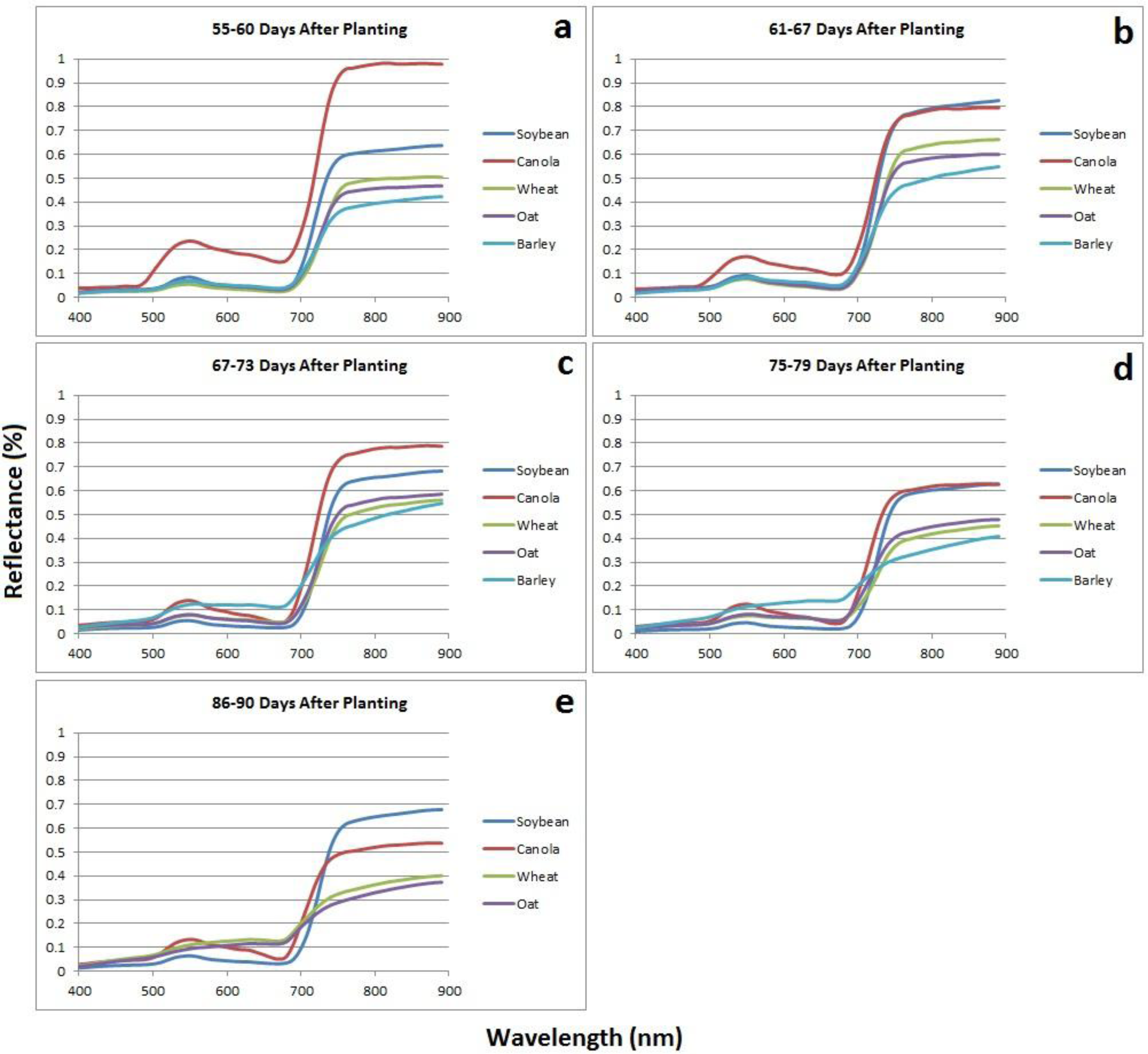
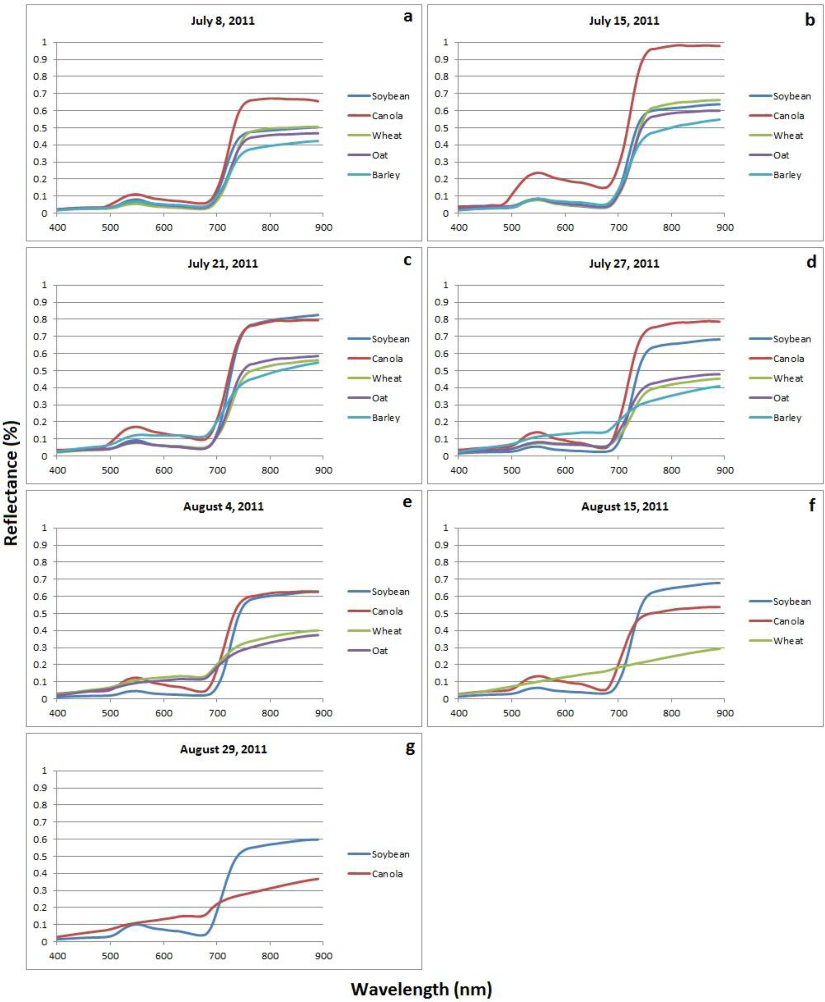
At 55–60 DAP (Figure 5a) canola is very distinguishable from the other crops hyperspectrally with high reflectance in the green and NIR portions of the spectrum as a result of flowering. The reflectance in the visible spectrum is similar for soybean, wheat, oats, and barley, however, soybean has a slightly higher reflectance in the NIR indicating denser vegetation canopy. At 61–67 DAP (Figure 5b), reflectance in the NIR for canola has dropped slightly, likely as a result of a change in plant structure due to the flower petals maturing and beginning to fall off. However, reflectance in the green and red portions of the spectrum for canola still remain slightly higher than for the other crops as there are still some yellow flowers on the plants. The yellow flowers of the canola crop cause increase reflectance in the green and red portions of the spectrum. Reflectance in the NIR for soybean has also reached its maximum of above 80%, which is likely a result of flowering and of the broad leaves reaching maturity before transferring their energy to pod production. At this stage in development, soybean has reached maturity and canopy coverage is dense allowing for very little light energy to pass through gaps in the canopy, ultimately resulting in strong reflectance back to the sensor. The spectral reflectance of the cereal crops (wheat, oats, and barley) are very similar with only minor variations in the NIR spectrum due to differences in the growth stage and the physical structure of the heads of each crop. Visually, 67–73 DAP (Figure 5c) appears to be one of the best times for crop separability. However, a thorough examination of the signatures reveals that although soybean and canola have clearly distinguished themselves from each other and from the rest of the crops hyperspectrally, the spectral reflectance of the cereal crops is very similar with overlap occurring in the NIR, red-edge and visible portions of the spectrum. At 75–79 DAP (Figure 5d) the cereal crops show good separation in the NIR, red-edge, and visible portions of the spectrum which are key areas for crop separability. The differences in spectral reflectance is attributed to the varying rates at which each crop begins to senesce and change from green to brown in colour. As the crops begin to senesce the structure of each crop changes dramatically and the canopy density quickly decreases.

The variable rates at which this occurs for each crop results in differences in spectral reflectance making crops more easily distinguishable. Barley has a shorter growing season and therefore has begun to senesce at a quicker rate, hence, the flattening of the spectral curve in relation to wheat and oats. The soybean and canola crops are still separable in the visible and red-edge portions of the spectrum. At 86–90 DAP (Figure 5e) soybean and canola still remain very distinguishable from each other as canola has begun to senesce and turn brown, whereas, soybean still remains relatively green in colour. The spectral curves of wheat and oats have begun to flatten as the crops senesce and die. At this stage, crops are still relatively distinguishable hyperspectrally, however, barley has been harvested which indicates that 86–90 DAP or later, may not be the most ideal time for crop separability. Visually, either 67–73 DAP or 75–79 DAP seem to be the most suitable times for crop separability.

4.1.2. Identification of Significant Bands for Crop Separability for DAP

An initial discriminant analysis was run using all bands for all crops to determine which bands were significant for crop separability. Classification accuracies for the bands initially selected as significant were high, ranging from 95.8% to 100%. However, a number of these initial bands were from similar parts of the electromagnetic spectrum (EMS) and, therefore, contained similar information. To reduce redundant information, similar bands were removed and a second discriminant analysis was run on the newly created set of bands.

The newly selected bands were chosen based primarily on where they were located in the EMS and how significant each band was in discriminating crops. For example, at 55–60 DAP, a total of 9 bands were identified as significant, after the initial discriminant analysis, including one violet band (B405), two blue bands (B455, B485), one green band (B535), one yellow band (B595), two red-edge bands (B705, B715), and two NIR bands (B765, B885). The blue band in the visible portion of the spectrum is highly influenced by atmospheric conditions through scattering [40] making it less desirable for crop discrimination; for this reason, bands B405, B455, and B485 were removed from further analysis. Band B535 was the only green band identified as significant and therefore was included for further analysis. The two red-edge bands identified as significant contained very similar information as they are very close to one another within the EMS. Discriminant analysis was run using each red-edge band and both generated similar classification results, however only one band was required for further analysis; for this reason, band B715 was chosen and band B705 was removed. Finally, both NIR bands were chosen for further analysis because band B765 is very close to the red-edge portion of the EMS while band B885 is well into the NIR spectrum; although both bands are located in the NIR spectrum, they were far enough apart to not contain very similar information. Bands located in transition zones from one part of the EMS to another (from blue to green, green to red, or red to NIR) are generally significant for crop discrimination especially the red-edge [8,31]. Heavy consideration was placed on identified red-edge bands as they are important for crop discrimination. In this way, the number of bands selected for further discriminant analysis was reduced from the initial 9 to a final of 4 for 55–60 DAP. The final sets of wavebands selected for crop discrimination are summarized in

Table 3. Selected bands for crop discrimination based on discriminant analysis for days after planting.

DAP	Crops	Selected Wavebands (nm)
48–52	soybean, canola	B465, B545
55–60	soybean, canola, wheat, oat, barley	B535, B715, B765, B885
61–67	soybean, canola, wheat, oat, barley	B465, B535, B715
67–73	soybean, canola, wheat, oat, barley	B535, B725
75–79	soybean, canola, wheat, oat, barley	B535, B675, B735, B885
86–90	soybean, canola, wheat, oat	B525, B695, B765, B825
97–104	soybean, canola, wheat	B665, B735, B765, B885

and the corresponding classification accuracies are summarized in

Table 4. Classification results (original and cross-validated) based on newly selected wavebands from initial discriminant analysis for days after planting.

DAP	Crop	Original		Cross-Validated		Misclassification
		Sample Size (/24)	Percent—Producer’s Accuracy	Count (/24)	Percent—Producer’s Accuracy
48–52	Soybean	24	100	24	100
	Canola	22	91.7	22	91.7	canola vs. soybean
55–60	Soybean	24	100	24	100
	Canola	24	100	24	100
	Wheat	21	87.5	21	87.5	wheat vs. oat
	Oat	23	95.8	23	95.8	oat vs. wheat
	Barley	24	100	24	100
61–67	Soybean	22	91.7	22	91.7	soybean vs. barley
	Canola	24	100	24	100
	Wheat	20	83.3	20	83.3	wheat vs. oat
	Oat	14	58.3	14	58.3	oat vs. wheat
	Barley	23	95.8	23	95.8	barley vs. soybean
67–73	Soybean	24	100	24	100
	Canola	24	100	24	100
	Wheat	20	83.3	20	83.3	wheat vs. oat
	Oat	20	83.3	19	79.2	oat vs. wheat
	Barley	22	91.7	22	91.7	barley vs. oat barley vs. wheat
75–79	Soybean	24	100	24	100
	Canola	24	100	24	100
	Wheat	24	100	24	100
	Oat	24	100	24	100
	Barley	24	100	23	95.8	barley vs. wheat
86–90	Soybean	24	100	24	100
	Canola	24	100	24	100
	Wheat	21	87.5	21	87.5	wheat vs. oat
	Oat	24	100	23	95.8	oat vs. wheat
97–104	Soybean	24	100	24	100
	Canola	21	87.5	21	87.5	canola vs. wheat
	Wheat	24	100	24	100

. Consequently, this method was used to determine smaller sets of bands for crop discrimination for all seven data acquisition dates throughout the growing season.

A total of 12 bands for Scenario 1 were deemed best suited for crop discrimination including B465, B525, B535, B545, B675, B695, B715, B725, B735, B765, B825, and B885. The significant bands vary by the number of DAP; however, there are some consistencies that should be noted. In general, almost every data acquisition date had a band in the green, red or red-edge and NIR portion of the EMS identified as significant. The most frequently occurring band was B535 in the green spectrum, which was identified as significant in four data acquisition dates. The second most frequently identified bands were B665 (red), B735 (red-edge), B765 (NIR), and B885 (NIR) each of which were identified twice.

The results for Scenario 1 indicate that the optimal time for crop discrimination is approximately 75–79 DAP. At this point in the growing season soybean, canola, wheat, oats and barley were at BBCH stage 73, 76, 75, 83, and 83, respectively (

Table 5. BBCH stages for all crops by days after planting (DAP).

DAP	Soybean		Canola		Wheat		Oat		Barley
	BBCH	Height (cm)	BBCH	Height (cm)	BBCH	Height (cm)	BBCH	Height (cm)	BBCH	Height (cm)
48–52	59	42	62	101	-	-	-	-	-	-
55–60	60	56	65	137	60	86	60	87	65	104
61–67	66	73	67	150	65	90	69	96	69	105
67–73	69	81	71	157	69	91	73	101	75	100
75–79	73	93	76	152	75	94	83	103	83	104
86–90	77	94	80	149	85	93	89	100	87	104
97–104	87	91	86	--	89	91	--	--	--	--

).

It is at this point that the difference in hyperspectral reflectance of crops is maximized and classification results were most accurate. Soybean, canola, wheat, and oat were classified at 100% accuracy, while barley was classified at 95.8% accuracy; only one barley variable was misclassified as wheat. The cereal crops seem most difficult to separate hyperspectrally due to similarities in plant structure. When the cereal crops mature and the heads of the plants begin to fill with seeds, differences in spectral reflectance are maximized due to changes in plant structure. In the later growth stages, the heads of the barley crop begin to lodge and produce hairs that protrude, ultimately increasing canopy coverage and spectral reflectance. The heads of the wheat crops enlarge but lodge only slightly, therefore, gaps between the rows of wheat are still present, which could decrease the amount of reflectance returning back to the sensor. The structure of the oat crop differs from wheat and barley in that there is not one single head that contains all the seeds. In fact, the seeds are dispersed along the main stem and along branches off the main stem ultimately increasing canopy density, which could explain the increased reflectance in the NIR portion of the spectrum in the later growth stages.

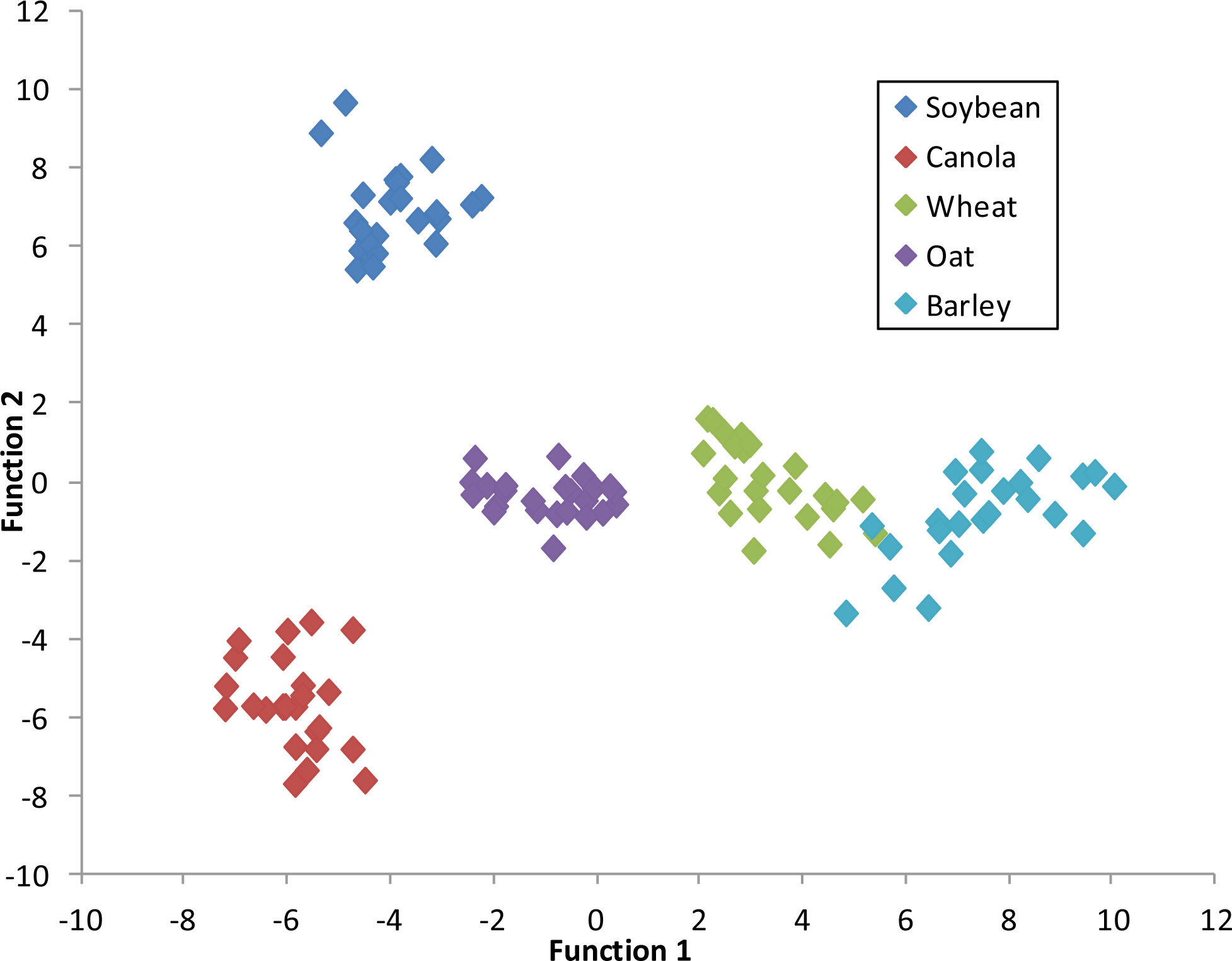
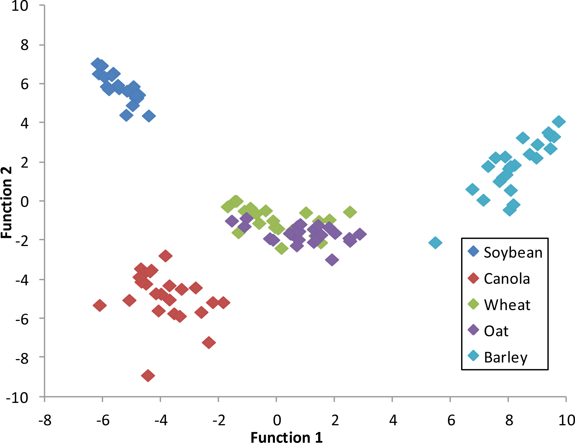
The wavebands identified as significant for crop discrimination at 74–79 DAP included band B535 (green), B675 (red), B735 (red-edge), and B885 (NIR). This suggests that if all crops are planted near the same date, 75–79 DAP would be the optimal time in the Northeastern Ontario growing season to capture a hyperspectral satellite image in order to most accurately distinguish these five cash crops. Figure 6 depicts a graph of the canonical discriminant function 1 versus function 2 at 75–79 DAP. Each class is clearly distinguishable from the other indicating a high degree of accuracy for crop classification based on the first two functions of the discriminant analysis.

4.2. Scenario 2—Specific Data Acquisition Dates

4.2.1. Interpretation of Spectral Reflectance for Specific Data Acquisition Dates

Scenario 2 involved comparing hyperspectral reflectance data at specific times throughout the growing season, regardless of the number of DAP and therefore represents a more realistic scenario. Hyperspectral reflectance data were acquired on 7 different dates throughout the growing season including 8 July, 15 July, 21 July, 27 July, 4 August, 15 August, and 29 August of 2011. Again, soybean and canola were planted approximately one week later than the cereal crops and were therefore slightly behind in growth stage. These planting dates are representative of those suggested by OMAFRA [36], and thus most likely to reoccur for this study area. The spectral signatures for all crops on each date of data collection are represented in Figure 7.

The interpretation of the spectral reflectance of crops for Figure 7a–g is very similar to that of Figure 5a–e. The difference between the spectral reflectance of crops in Figure 7 compared to those in Figure 5 is principally based on timing. For example, increased spectral reflectance in the visible and NIR spectrum for canola is very evident at 55–60 DAP (Figure 5a) for Scenario 1 as well as on 15 July (Figure 7b) for Scenario 2. In fact, these two spectral signatures for canola are identical with the observed increased reflectance attributed to the emergence of yellow flowers at this time. Consequently, the spectral signatures for each crop in Figure 7 can be interpreted the same way as for Figure 5. It is the different combination of spectral signatures being compared, based on the timing of each scenario, which results in different bands being identified as significant for crop separability.

4.2.2. Identification of Significant Bands for Crop Separability for Specific Acquisition Dates

Using the same method as in Scenario 1, an initial discriminant analysis was run using all bands for all crops to determine which bands were significant for crop discrimination. Classification accuracies for the bands initially selected as significant were high, ranging from 95.8% to 100%. However, a number of these initial bands were from similar parts of the electromagnetic spectrum (EMS) and therefore contained similar information. To reduce redundant information, similar bands were removed, using the same methodology as in Scenario 1, and a second discriminant analysis was run using the newly created set of bands.

Again, bands that contained redundant information or were deemed unsuitable for crop discrimination based on their location in the EMS were removed from further analysis and consideration was given to bands located in transition zones, especially in the red-edge portion of the spectrum.

Table 6. Selected bands for crop discrimination based on discriminant analysis for specific dates.

Date	Crops	Selected Wavebands (nm)
8 July	soybean, canola, wheat, oat, barley	B495, B645, B725, B815
15 July	soybean, canola, wheat, oat, barley	B495, B525, B645, B705, B745, B895
21 July	soybean, canola, wheat, oat, barley	B535, B725
27 July	soybean, canola, wheat, oat, barley	B485, B515, B675, B705, B755
4 August	soybean, canola, wheat, oat, barley	B535, B625, B725, B825
15 August	soybean, canola, wheat	B665, B725, B755, B895
29 August	soybean, canola, wheat	B665, B745

represents the bands selected for crop discrimination for specific dates and the corresponding classification results for the selected wavebands are represented in

Table 7. Classification results (original and cross-validated) based on newly selected wavebands from initial discriminant analysis for specific dates during the growing season.

Date	Crop	Original		Cross-Validated		Misclassification
		Sample Size (/24)	Percent—Producer’s Accuracy	Count (/24)	Percent—Producer’s Accuracy
8 July	Soybean	24	100	24	100
	Canola	24	100	23	95.8	canola vs. soybean
	Wheat	23	95.8	21	87.5	wheat vs. oat
	Oat	19	79.2	17	70.8	oat vs. wheat (1) oat vs. barley (6)
	Barley	22	91.7	22	91.7	barley vs. oat
15 July	Soybean	24	100	24	100
	Canola	24	100	24	100
	Wheat	24	100	24	100
	Oat	22	91.7	22	91.7	oat vs. wheat
	Barley	24	100	24	100
21 July	Soybean	23	95.8	23	95.8	soybean vs. oat
	Canola	22	91.7	22	91.7	canola vs. barley
	Wheat	22	91.7	22	91.7	wheat vs. oat
	Oat	18	75	18	75	oat vs. wheat
	Barley	21	87.5	20	83.3	barley vs. oat (1) barley vs. wheat (3)
27 July	Soybean	24	100	24	100
	Canola	24	100	24	100
	Wheat	24	100	24	100
	Oat	20	83.3	20	83.3	oat vs. wheat
	Barley	24	100	24	100
4 August	Soybean	24	100	24	100
	Canola	24	100	24	100
	Wheat	17	70.8	16	66.7	wheat vs. oat
	Oat	18	75	18	75	oat vs. wheat
15 August	Soybean	24	100	24	100
	Canola	24	100	24	100
	Wheat	24	100	24	100
29 August	Soybean	24	100	24	100
	Canola	24	100	24	100

.

Similar to Scenario 1, the classification accuracies of the second set of wavebands dropped slightly in comparison to the initial discriminant analysis. However, the objective is to reduce the number of wavebands used to classify crops as much as possible while still maintaining a relatively high degree of classification accuracy.

A total of 16 bands were identified as most suitable for crop discrimination in Scenario 2 including B485, B495, B515, B525, B535, B625, B645, B665, B675, B705, B725, B745, B755, B815, B825, and B895. Again the significant bands vary by date and patterns were again apparent. Every date had a band in the red-edge portion of the EMS identified as significant and, with the exception of 15 August and 29 August, every date had a band in the green portion of the EMS identified as significant. All dates but 21 July identified a band in the NIR portion of the spectrum as significant and three dates (8 July, 15 July, and 27 July) identified a band in the transition zone between blue and green portions of the EMS. The most frequently occurring band was B725 in the red-edge portion of the spectrum which was identified as significant for four dates. The second most frequently occurring significant bands were B495 (blue/green), B535 (green), B645 (red), B665 (red), B705 (red-edge), B725 (red-edge), B755 (red-edge/NIR), and B895 (NIR) all of which were identified at least twice.

The results of this scenario indicate that the optimal time for crop discrimination for Scenario 2 is around 27 July when soybean, canola, wheat, oat, and barley are at BBCH stage 69, 71, 75, 83, and 83 respectively which are similar to the results for Scenario 1. For 27 July, the classification results were 100% for all crops except oat, which misclassified four variables as wheat. The wavebands identified as significant for crop discrimination on 27 July included B485 (blue/green), B515 (green), B675 (red), B705 (red-edge), and B755 (red-edge/NIR). This suggests that late July would be the optimal time in the Northeastern Ontario growing season to capture a hyperspectral satellite image in order to most accurately distinguish these five cash crops. Figure 8 depicts a graph of the canonical discriminant function 1 versus function 2 for 27 July. With the exception of wheat and oat, all of the crops are clearly distinguishable from each other indicating a high degree of accuracy for crop classification using the first two functions. Figure 9 depicts a graph of function 3 versus for function 4 and shows good separation between wheat and oat. This indicates that all crops can be separated with a high degree of accuracy using the four functions of discriminant analysis. It should also be noted that both 15 August and 29 August classified all crops with 100% accuracy, making them excellent dates for crop discrimination; however, on August 15 oat and barley had already been harvested and, on 29 August, the only remaining crops were soybean and canola.

4.3. General Discussion Based on Scenario 1 and Scenario 2

Based on the results from both Scenario 1 and Scenario 2, it is suggested that the optimal time for distinguishing crops hyperspectrally, whether using DAP or the specific date approach, occurs when cereal crops, soybean and canola are between the BBCH stages of 75 and 83, 69 and 73, and 71 and 76, respectively. The aforementioned growth stages represent the period of the growing season in which all five crops begin fruit development, suggesting that the late vegetative growth stages are optimal for crop separability using hyperspectral remote sensing. Early vegetative growth stages (leaf development and tillering) are less desirable for crop separation as the plants are significantly small, resulting in large patches of soil affecting the reflectance of electromagnetic energy. Moreover, during the middle growth stages (stem elongation, booting, and inflorescence) it is very difficult to distinguish cereal crops visually. Prior to the emergence of the heads of cereal crops, wheat, oat, and barley are almost indistinguishable. Canola and soybean are easily distinguishable from cereal crops at all growth stages, however they are less easily distinguishable from each other at the very early growth stages. The fact that most of the crops in this study are only distinguishable visually in the middle to late BBCH growth stages reiterates the importance for optimal hyperspectral separation of crops later in the growing season. Consequently, it is recommended that satellite images be acquired during the key periods identified in this study in order to maximize the usefulness of that imagery for crop classification.

5. Conclusion

Crops in Northeastern Ontario can be distinguished with hyperspectral data captured by an ASD FieldSpec Handheld Portable Spectroradiometer with a relatively high degree of accuracy and confidence. The results indicate that the optimal time for crop discrimination in this area is 75–79 DAP (if all crops are planted at the same time) or in late July assuming crops were planted according to guidelines set forth by OMAFRA. At this point in the growing season the difference in hyperspectral reflectance of soybean, canola, wheat, oats, and barley is maximized allowing for accurate discrimination of these crops. It should be noted, however, that classification accuracies were relatively high throughout the entire growing season using a set of wavebands identified as significant for crop discrimination through stepwise discriminant analysis, implying that a handheld spectroradiometer could be used to discriminate crops with relative accuracy at any point in the growing season.

This study resulted in recommending a total of 23 optimal bands in the 400–900 nm range to discriminate soybean, canola, wheat, oat and barley in Northeastern Ontario, Canada. These bands include B465, B485, B495, B515, B525, B535, B545, B625, B645, B665, B675, B695, B705, B715, B725, B735, B745, B755, B765, B815, B825, B885, and B895. A total of 12 bands were identified for Scenario 1 and a total of 16 bands for Scenario 2. The locations of the identified bands in the EMS are as follows: two blue, five green, five red, six red-edge, and five NIR.

In summary, the results of this study have indicated that hyperspectral reflectance data collected using a handheld portable spectroradiometer, with a spectral range of 400–900 nm, is well suited for crop discrimination in Northeastern Ontario. Future researchers could consider the bands and timeframes identified in this study for specific agricultural applications such as crop discrimination.

References

1. An Overview of the Canadian Agriculture and Agri-Food System 2013. Avaliable online: http://www.agr.gc.ca/eng/about-us/publications/economic-publications/alphabetical-listing/an-overview-of-the-canadian-agriculture-and-agri-food-system-2013/?id=1331319696826 (accessed on 1 July 2013).
2. Haboudane, D.; Miller, J.R.; Pattey, E.; Zarco-Tejada, P.; Strachan, I.B. Hyperspectral vegetation indices and novel algorithms for predicting green LAI of crop canopies: Modeling and validation in the context of precision agriculture. Remote Sens. Environ 2004, 90, 337–352. [Google Scholar]
3. Thenkabail, P.S.; Enclona, E.A.; Ashton, M.S.; van Der Meer, B. Accuracy assessments of hyperspectral waveband performance for vegetation analysis applications. Remote Sens. Environ 2004, 91, 345–376. [Google Scholar]
4. Gray, C.J.; Shaw, D.R.; Bruce, L.M. Utility of hyperspectral reflectance for differentiating soybean (Glycine max) and six weed species. Weed Technol 2009, 23, 108–119. [Google Scholar]
5. Martin, M.P.; Barreto, L.; Riano, D.; Fernandez-Quintanilla, C.; Vaughan, P. Assessing the potential of hyperspectral remote sensing for the discrimination of grassweeds in winter cereal crops. Int. J. Remote Sens 2011, 32, 49–67. [Google Scholar]
6. Lin, W.-S.; Yang, C.-M.; Kuo, B.-J. Classifying cultivars of rice (Oryza sativa L.) based on corrected canopy reflectance spectra data using the orthogonal projections to latent structures (O-PLS) method. Chemometr. Intell. Lab. Syst 2012, 115, 25–36. [Google Scholar]
7. Pena-Barragan, J.M.; Lopez-Granados, F.; Jurado-Exposito, M.; Carcia-Torres, L. Spectral discrimination of Ridolfia segetum and sunflower as affected by phenological stage. Weed Res 2006, 46, 10–21. [Google Scholar]
8. Zhang, H.; Lan, Y.; Suh, C.P.; Westbrook, J.K.; Lacey, R.; Hoffmann, W.C. Differentiation of cotton from other crops at different growth stages using spectral properties and discriminant analysis. Trans. ASABE 2012, 55, 1623–1630. [Google Scholar]
9. Shibayama, M.; Tsuyoshi, A. Estimating grain yield of maturing rice canopies using high spectral resolution reflectance measurements. Remote Sens. Environ 1991, 36, 45–53. [Google Scholar]
10. Blackburn, G.A.; Steele, C.M. Towards the remote sensing of matorral vegetation physiology: Relationships between spectral reflectance, pigment, and biophysical characteristics of semiarid bush land canopies. Remote Sens. Environ 1999, 70, 278–292. [Google Scholar]
11. McGwire, K.; Minor, T.; Fenstermarker, L. Hyperspectral mixture modeling for quantifying sparse vegetation cover in arid environments. Remote Sens. Environ 2000, 72, 360–374. [Google Scholar]
12. Thenkabail, P.S. Biophysical and yield information for precision farming from near-real-time and historical Landsat TM images. Int. J. Remote Sens 2003, 24, 2879–2904. [Google Scholar]
13. Manjunath, K.R.; Ray, S.S.; Panigrahy, S. Discrimination of spectrally-close crops using ground-based hyperspectral data. J. Indian Soc. Remote Sens 2011, 39, 599–602. [Google Scholar]
14. Broge, N.H.; Mortensen, J.V. Deriving green crop area index and canopy chlorophyll density of winter wheat from spectral reflectance data. Remote Sens. Environ 2002, 81, 45–57. [Google Scholar]
15. Darvishzadeh, R.; Skidmore, A.; Schlerf, M.; Atzberger, C.; Corsi, F.; Cho, M. LAI and chlorophyll estimation for a heterogeneous grassland using hyperspectral measurements. ISPRS J. Photogramm. Remote Sens 2008, 63, 409–426. [Google Scholar]
16. Estimation of Leaf Area Index Using Ground Spectral Measurements over Agriculture Crops: Prediction Capability Assessment of Optical Indices. Available online: http://citeseerx.ist.psu.edu/viewdoc/download?doi=10.1.1.158.6391&rep=rep1&type=pdf (accessed on 17 January 2014).
17. Muller, K.; Bottcher, U.; Meyer-Schatz, F.; Kage, H. Analysis of vegetation indices derives from hyperspectral reflection measurements for estimating crop canopy parameters of oilseed rape (Brassica napus L.). Biosys. Eng 2008, 101, 172–182. [Google Scholar]
18. Zhao, D.H.; Li, J.L.; Qi, J.G. Identification of red and NIR spectral regions and vegetative indices for discrimination of cotton nitrogen stress and growth stage. Comput. Electron. Agr 2005, 48, 155–169. [Google Scholar]
19. Broge, N.H.; Leblanc, E. Comparing prediction power and stability of broadband and hyperspectral vegetation indices for estimation of green leaf area index and canopy chlorophyll density. Remote Sens. Environ 2001, 76, 156–172. [Google Scholar]
20. Haboudane, D.; Miller, J.R.; Tremblay, N.; Zarco-Tejada, P.J.; Dextraze, L. Integrated narrow-band vegetation indices for prediction of crop chlorophyll content for application to precision agriculture. Remote Sens. Environ 2002, 81, 416–426. [Google Scholar]
21. Nidamanuri, R.R.; Zbell, B. Transferring spectral libraries of canopy reflectance for crop classification using hyperspectral remote sensing data. Biosyst. Eng 2011, 110, 231–246. [Google Scholar]
22. Rao, N.R. Development of a crop-specific spectral library and discrimination of various agricultural crop varieties using hyperspectral imagery. Int. J. Remote Sens 2008, 29, 131–144. [Google Scholar]
23. Zhang, H.; Hinze, L.L.; Lan, Y.; Westbrook, J.K.; Hoffmann, W.C. Discriminating among cotton cultivars with varying leaf characteristics using hyperspectral radiometry. Trans. ASABE 2012, 55, 275–280. [Google Scholar]
24. Mahesh, S.; Manickavasagan, A.; Jayas, D.S.; Paliwal, J.; White, N.D.G. Feasibility of near-infrared hyperspectral imaging to differentiate Canadian wheat classes. Biosyst. Eng 2008, 101, 50–57. [Google Scholar]
25. Thenkabail, P.S.; Smith, R.B.; De Pauw, E. Evaluation of narrowband and broadband vegetation indices for determining optimal hyperspectral wavebands for agricultural crop characterization. Photogramm. Eng. Remote Sens 2002, 68, 607–621. [Google Scholar]
26. Jorgensen, R.R.; Hansen, P.M.; Bro, R. Exploratory study of winter wheat reflectance during vegetative growth using three-mode component analysis. Int. J. Remote Sens 2006, 27, 919–937. [Google Scholar]
27. Wang, Y.; Wang, F.; Huang, J.; Wang, X.; Liu, Z. Validation of artificial neural network techniques in the estimation of nitrogen concentration in rape using canopy hyperspectral reflectance data. Int. J. Remote Sens 2009, 30, 4493–4505. [Google Scholar]
28. Yang, X.; Huang, J.; Wang, J.; Wang, X.; Liu, Z. Estimation of vegetation biophysical parameters by remote sensing using radial basis function neural network. J. Zhejiang Univ. Sci. A 2007, 8, 883–895. [Google Scholar]
29. Liu, Z.-Y.; Wu, H.-F.; Huang, J.-F. Application of neural networks to discriminate fungal infection levels in rice panicles using hyperspectral reflectance and principal components analysis. Comput. Electron. Agr 2010, 72, 99–106. [Google Scholar]
30. Pena-Barragan, J.; Ngugi, M.K.; Plant, R.E.; Six, J. Object-based crop identification using multiple vegetation indices, textural features and crop phenology. Remote Sens. Environ 2011, 115, 1301–1316. [Google Scholar]
31. Thenkabail, P.S.; Smith, R.B.; De Pauw, E. Hyperspectral vegetation indices and their relationships with agricultural crop characteristics. Remote Sens. Environ 2000, 71, 158–182. [Google Scholar]
32. Song, S.; Gong, W.; Zhu, B.; Huang, X. Wavelength selection and spectral discrimination for paddy rice, with laboratory measurements of hyperspectral leaf reflectance. ISPRS J. Photogramm. Remote Sens 2011, 66, 672–682. [Google Scholar]
33. Zhang, C.; Kovacs, J.M.; Wachowiak, M.; Flores-Verdugo, F. Relationship between hyperspectral measurements and mangrove leaf nitrogen concentrations. Remote Sens 2013, 5, 891–908. [Google Scholar]
34. Zhao, D.H.; Huang, L.; Li, J.; Qi, J. A comparative analysis of broadband and narrowband derived vegetation indices in predicting LAI and CCD of a cotton canopy. ISPRS J. Photogramm. Remote Sens 2007, 62, 25–33. [Google Scholar]
35. The Corporation of the Municipality of West Nipissing. Agriculture in West Nipissing. Available online: http://www.westnipissing.ca/economic-development-e/agriculture (accessed on 15 May 2012).
36. Brown, C. Agronomy Guide for Field Crops; Queens Printer for Ontario: Toronto, ON, Canada, 2009. [Google Scholar]
37. Bannari, A.; PacheCo, A.; Staenz, K.; McNairn, H.; Omari, K. Estimating and mapping crop residues cover on agricultural lands using hyperspectral and IKONOS data. Remote Sens. Environ 2006, 104, 447–459. [Google Scholar]
38. Haché, C.; Shibusawa, S.; Sasao, A.; Suhama, T.; Sah, B.P. Field-derived spectral characteristics to classify conventional and conservation agricultural practices. Comput. Electron. Agr 2007, 57, 47–61. [Google Scholar]
39. Flores-de-Santiago, F.; Kovacs, J.M.; Flores-Verdugo, F. The influence of seasonality in estimating mangrove leaf chlorophyll-a content from hyperspectral data. Wetl. Ecol. Manag 2013, 21, 193–207. [Google Scholar]
40. Jensen, J.R. Remote Sensing of the Environment: An Earth Resource Perspective; Prentice Hall: Upper Saddle River, NJ, USA, 2006. [Google Scholar]
Figure 1. Study area located near Verner, Ontario in West Nipissing. The background is a WorldView-2 image (natural color composite) acquired 2 July 2011.
Remotesensing 06 00925f1
Figure 2. Canola at key growth stages (BBCH) across the growing season at specific number of days after planting (DAP).
Remotesensing 06 00925f2
Figure 3. Subplot design for the hyperspectral data collection in each field.
Remotesensing 06 00925f3
Figure 4. Preparing the ASD Inc. FieldSpec HandHeld Visible/Near Infrared portable spectroradiometer for measurements in an oat (Avena sativa) field in West Nipissing, Ontario, Canada.
Remotesensing 06 00925f4
Figure 5. Spectral signatures for all crops organized by number of days after planting. (a) Spectral signatures for all crops at 55–60 DAP. (b) Spectral signatures for all crops at 61–67 DAP. (c) Spectral signatures for all crops at 67–73 DAP. (d) Spectral signatures for all crops at 75–79 DAP. (e) Spectral signatures for soybean, canola, wheat and oat crops at 86–90 DAP.
Remotesensing 06 00925f5
Figure 6. Canonical discriminant function 1 versus function 2 for 75–79 days after planting.
Remotesensing 06 00925f6
Figure 7. Spectral signatures for all crops organized by date of collection. (a) Spectral signatures for all crops on 8 July 2011. (b) Spectral signatures for all crops on 15 July 2011. (c) Spectral signatures for all crops on 21 July 2011. (d) Spectral signatures for all crops on 27 July 2011. (e) Spectral signatures for soybean, canola, wheat and oat crops on 4 August 2011. (f) Spectral signatures for soybean, canola and wheat crops on 15 August 2011. (g) Spectral signatures for soybean and canola crops on 29 August 2011.
Remotesensing 06 00925f7
Figure 8. Canonical discriminant function 1 versus function 2 for 27 July 2011.
Remotesensing 06 00925f8
Figure 9. Canonical discriminant function 3 versus function 4 for 27 July 2011.
Remotesensing 06 00925f9