Article

An Assessment of Polynomial Regression Techniques for the Relative Radiometric Normalization (RRN) of High-Resolution Multi-Temporal Airborne Thermal Infrared (TIR) Imagery

1
The Department of Geography, University of Calgary, 2500 University Dr. NW, Calgary, AB T2N 1N4, Canada
2
Canadian Pacific Railway, 7550 Ogden Dale Road S.E. Calgary, AB T2C 4X9, Canada
3
The Department of Physics & Astronomy, University of Alabama, Box 870324, Tuscaloosa, AL 35487-0324, USA
*
Author to whom correspondence should be addressed.
Remote Sens. 2014, 6(12), 11810-11828; https://doi.org/10.3390/rs61211810
Submission received: 10 September 2014 / Revised: 8 November 2014 / Accepted: 18 November 2014 / Published: 27 November 2014
(This article belongs to the Special Issue Recent Advances in Thermal Infrared Remote Sensing)

Abstract

:
Thermal Infrared (TIR) remote sensing images of urban environments are increasingly available from airborne and satellite platforms. However, limited access to high-spatial resolution (H-res: ~1 m) TIR satellite images requires the use of TIR airborne sensors for mapping large complex urban surfaces, especially at micro-scales. A critical limitation of such H-res mapping is the need to acquire a large scene composed of multiple flight lines and mosaic them together. This results in the same scene components (e.g., roads, buildings, green space and water) exhibiting different temperatures in different flight lines. To mitigate these effects, linear relative radiometric normalization (RRN) techniques are often applied. However, the Earth’s surface is composed of features whose thermal behaviour is characterized by complexity and non-linearity. Therefore, we hypothesize that non-linear RRN techniques should demonstrate increased radiometric agreement over similar linear techniques. To test this hypothesis, this paper evaluates four (linear and non-linear) RRN techniques, including: (i) histogram matching (HM); (ii) pseudo-invariant feature-based polynomial regression (PIF_Poly); (iii) no-change stratified random sample-based linear regression (NCSRS_Lin); and (iv) no-change stratified random sample-based polynomial regression (NCSRS_Poly); two of which (ii and iv) are newly proposed non-linear techniques. When applied over two adjacent flight lines (~70 km2) of TABI-1800 airborne data, visual and statistical results show that both new non-linear techniques improved radiometric agreement over the previously evaluated linear techniques, with the new fully-automated method, NCSRS-based polynomial regression, providing the highest improvement in radiometric agreement between the master and the slave images, at ~56%. This is ~5% higher than the best previously evaluated linear technique (NCSRS-based linear regression).

Graphical Abstract

1. Introduction

Remote sensing technology has been widely used to monitor the Earth’s surface from satellite, piloted fixed-wing aircraft and UAS (unmanned aircraft system) platforms, by recording the radiant energy emitted or reflected from the Earth’s surface. However, these images are strongly influenced by the Sun-surface-sensor geometry, sensor characteristics, atmospheric absorption and scattering and microclimatic conditions that introduce noise within the sensor recorded radiant energy [1,2,3]. As the influence of these factors vary over time, a ground object viewed at different times or by different sensors tends to exhibit different sensor measurements. Thus, to use multiple datasets collected at different times or from different sources, it is necessary to either retrieve the surface radiance by applying suitable atmospheric corrections to each image (i.e., absolute atmospheric correction) or normalize the radiance values to a standard set of conditions (i.e., relative radiometric normalization) [4].
Absolute radiometric correction techniques aim to extract absolute surface radiances using sensor calibration parameters and atmospheric properties at the time of data acquisition [5]. However, it is often difficult to collect the necessary ancillary data (i.e., atmospheric characteristics and sensor calibration parameters) for absolute corrections due to the (financial and logistic) costs involved, as well as the lack of historical weather data. Whereas, relative radiometric normalization (RRN) techniques aim to reduce radiometric differences among multi-temporal images by normalizing the radiometric properties of the slave image(s) to a master image, so that it appears as if all of the images were acquired using the same sensor and under the same environmental conditions as the master [6]. A master image is the reference image that is considered to be radiometrically “correct”. Slave images (one or more images in an image set) are considered to have radiometric distortion; thus, they are normalized “to” the master image.
RRN techniques are often preferred over absolute techniques, because they require no in situ data, and they are able to take into account all forms of noise generated from the atmosphere, sensor, microclimate and other possible sources in a single straightforward process [7]. As a consequence, relative techniques have been widely used for the normalization of multi-temporal multispectral imagery [6,8,9,10].
However, there are few reports of RRN techniques applied to high resolution airborne thermal infrared (TIR) imagery, as they are typically applied to satellite-based TIR imagery acquired at moderate to low spatial resolution (60 m to 1 km), where there are fewer details to compare, as each pixel in the image has already been regularized. For example, Warner and Chen [11] applied RRN to suppress the effects of solar heating and topography in daytime Landsat TIR data. They evaluated three RRN techniques and concluded that these methods were able to demonstrate improved radiometry of the original dataset. Scheidt et al. [12] mosaicked night-time ASTER TIR data by automatically selecting pseudo-invariant features (PIFs) from scene overlaps and then fitting the PIFs in a linear regression model. More recently, Rahman et al. [13] recognized the need to validate RRN techniques on high resolution (H-res) multi-temporal TIR imagery and evaluated four RRN techniques (typically used for multispectral data) on multiple flight lines of TABI-1800 (Thermal Airborne Broadband Imager) data (at a 50-cm spatial resolution). These included: (i) histogram matching; (ii) pseudo-invariant feature (PIF)-based linear regression; (iii) PIF-based Theil-Sen regression (the Theil-Sen [14,15] estimator is a robust linear regression model that uses the median of pairwise slopes as an estimator of the slope parameter of the correlation between two datasets [16]); and (iv) no-change stratified random sample (NCSRS)-based linear regression. Their study showed that two of these methods (i and iv) visually and statistically performed better than the others, improving the radiometric agreement between multi-temporal TIR flight lines by ~50%.
Each of the RRN techniques used in these previously noted studies were linear in nature. That is, for the purpose of simplifying analysis, it was assumed that the thermal properties of the different surface types were linearly correlated. However, in reality, the Earth’s surface is a complex mixture of natural and man-made features exhibiting very different, often non-linear thermal properties [17]. For example, if water and rock are heated for a constant time under identical environmental settings, the rock temperature will rise much quicker than the water due to its lower thermal capacity [18]. Similarly, Oke [19] conducted an extensive study on the thermal characteristics of different surfaces of the Earth. His results demonstrated a clear difference in the cooling rates of different surfaces, including snow, peat soil, sandy soil, clay soil, water, rocks, farmland and woods from sunset to sunrise. A more recent study [20] also examined the daytime thermal behaviour of urban surfaces, which revealed nonlinear thermal relationships (over time) among different construction materials, including granulite, mixed asphalt, bright concrete and dark concrete. Thus, assuming simple linear thermal relationships among different types of complex surfaces is expected to produce sub-optimal results. As a result, we hypothesize that non-linear RRN techniques should demonstrate increased radiometric agreement over complex urban surfaces, compared to similar linear techniques. To test this hypothesis, the objective of this paper is to evaluate the two most suitable linear techniques for the RRN of airborne TIR imagery, as recently described by Rahman et al. [13], against two newly proposed polynomial techniques (which are expected to better suit the thermal complexity of urban surfaces) and to evaluate them visually and statistically. To achieve this objective, the following section (Section 2) describes the study area, datasets and the RRN techniques used. This is proceeded by a thorough discussion of the results (Section 3) and the lessons learned (Section 4).

2. Methods

In this section, we introduce the study area and the dataset. We then describe the four relative radiometric normalization (RRN) techniques evaluated in this study.

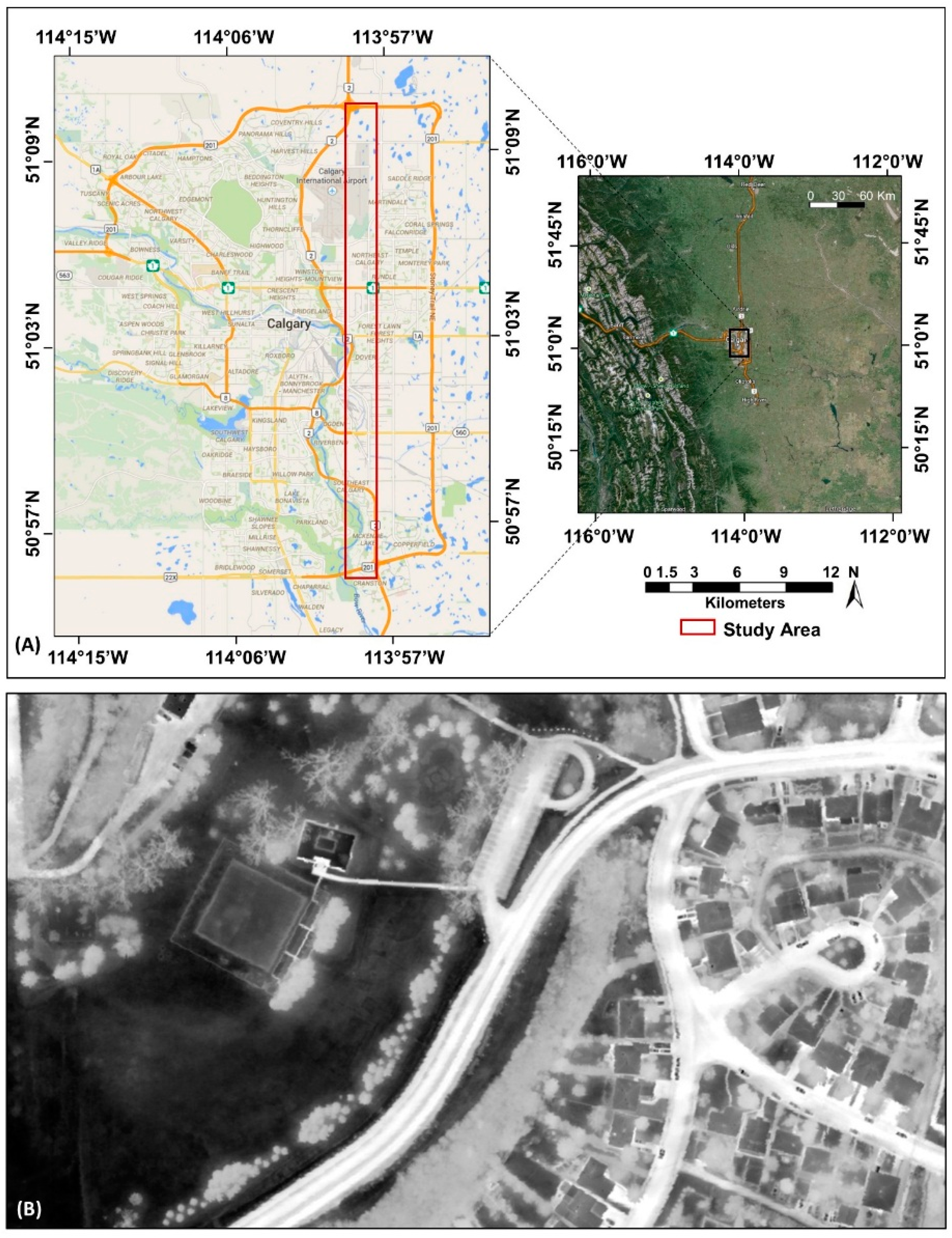
2.1. Study Area and Dataset

Our study area represents a (~70 km2) portion of The City of Calgary, Alberta, Canada, composed of two adjacent TABI-1800 TIR flight lines (Figure 1A), each ~0.9 km wide by 39 km long with ~30% overlap between them. The City of Calgary is situated approximately 80 km east of the front ranges of the Canadian Rockies mountain range and, as a modern metropolitan center, is composed of a variety of urban landscape features (Figure 1B). The TABI-1800 (Thermal Airborne Broadband Imager) is an H-res TIR airborne sensor that has a swath-width of 1800 pixels, which it collects in a single channel (3.7–4.8 µm spectral range). It has an instantaneous field of view (IFOV) of 0.405 milliradians and a field of view (FOV) of ±40 degrees with a 14-bit dynamic range. The sensor’s radiometric accuracy is 0.05 °C, and it is able to collect data at 90–100 frames per second. The data for this project were acquired between 2:00 and 3:00 am on 13 May 2012, at a 50-cm spatial resolution and were ortho-rectified using a 10-m DEM (digital elevation model). The reported (horizontal) geometric accuracy of the dataset is ±1 m.
Figure 1. (A) The City of Calgary map, displaying the location of the two TABI-1800 flight lines used in this study. (B) An example of TABI-1800 imagery (at 50 cm pixels) within the study area, detailing the urban complexity resulting from roads, buildings, trees, green space, etc. Bright locations are warm, and dark locations are cool.
Remotesensing 06 11810 g001

2.2. Relative Radiometric Normalization

The RRN methods evaluated in this study include: (i) histogram matching (HM); (ii) pseudo-invariant feature-based polynomial regression (PIF_Poly); (iii) no-change stratified random sample-based linear regression (NCSRS_Lin); and (iv) no-change stratified random sample-based polynomial regression (NCSRS_Poly). All algorithms were written in-house using the Interactive Data Language (IDL 8.0), were applied to the same datasets and were performed using the same workstation (an Intel(R) Core(TM) i7–2600, running Windows Server 2008 (64 bit) on a Quad Core CPU at 3.40 GHz, 16 GB RAM).
As we only have 30% overlap (max) between the master and the slave images, we (i) first extract the overlap sections from both flight lines; as this represents the same land area observed at two different acquisition times. Next, (ii) we develop all RRN methods based on these overlaps, then (iii) we apply the RRN methods exclusively to the (entire) slave flight line, thus normalizing it to the master. The RRN methods used in this study are briefly described below.

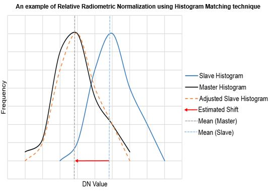
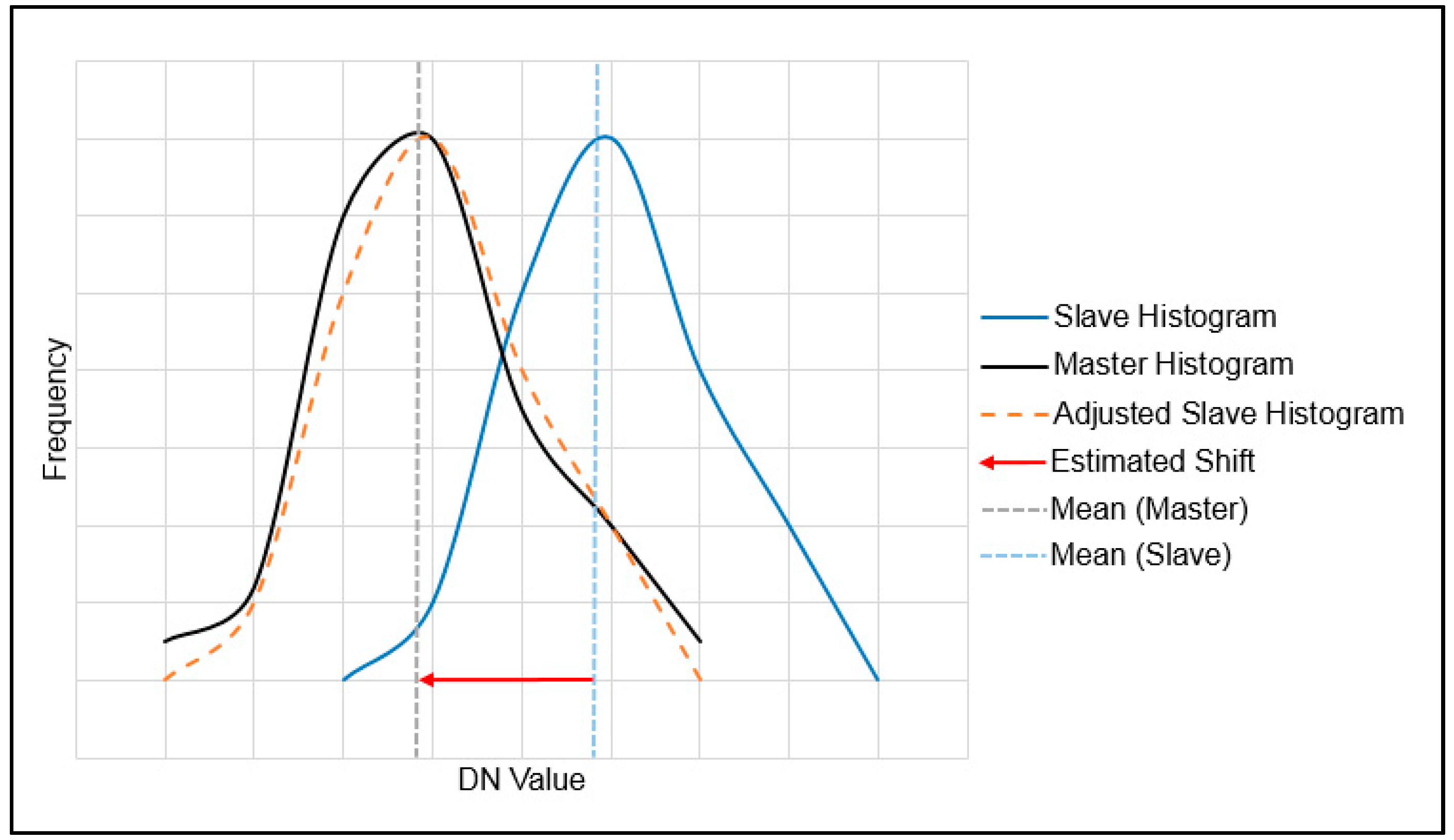
2.2.1. Histogram Matching

Histogram matching (HM) is described as matching the histogram of the slave image to that of the master image, so that their apparent distribution of the digital number (DN) values becomes closer [21]. The simplest way to perform HM is to create the histogram of the master and the slave images, then calculate the mean difference using Equation (1) and use it to shift (a.k.a. normalize) the slave histogram to the master [13]. Figure 2 displays a hypothetical example of the HM technique.
M D =   1 n i = 1 i = n ( y i   x i )
where, M D = the mean difference, n = the number of pixels, x i = the value of pixel i in the slave image and y i = the value of pixel i in the master image.
Figure 2. A hypothetical example of radiometric normalization using the histogram matching technique. DN (digital number).
Remotesensing 06 11810 g002

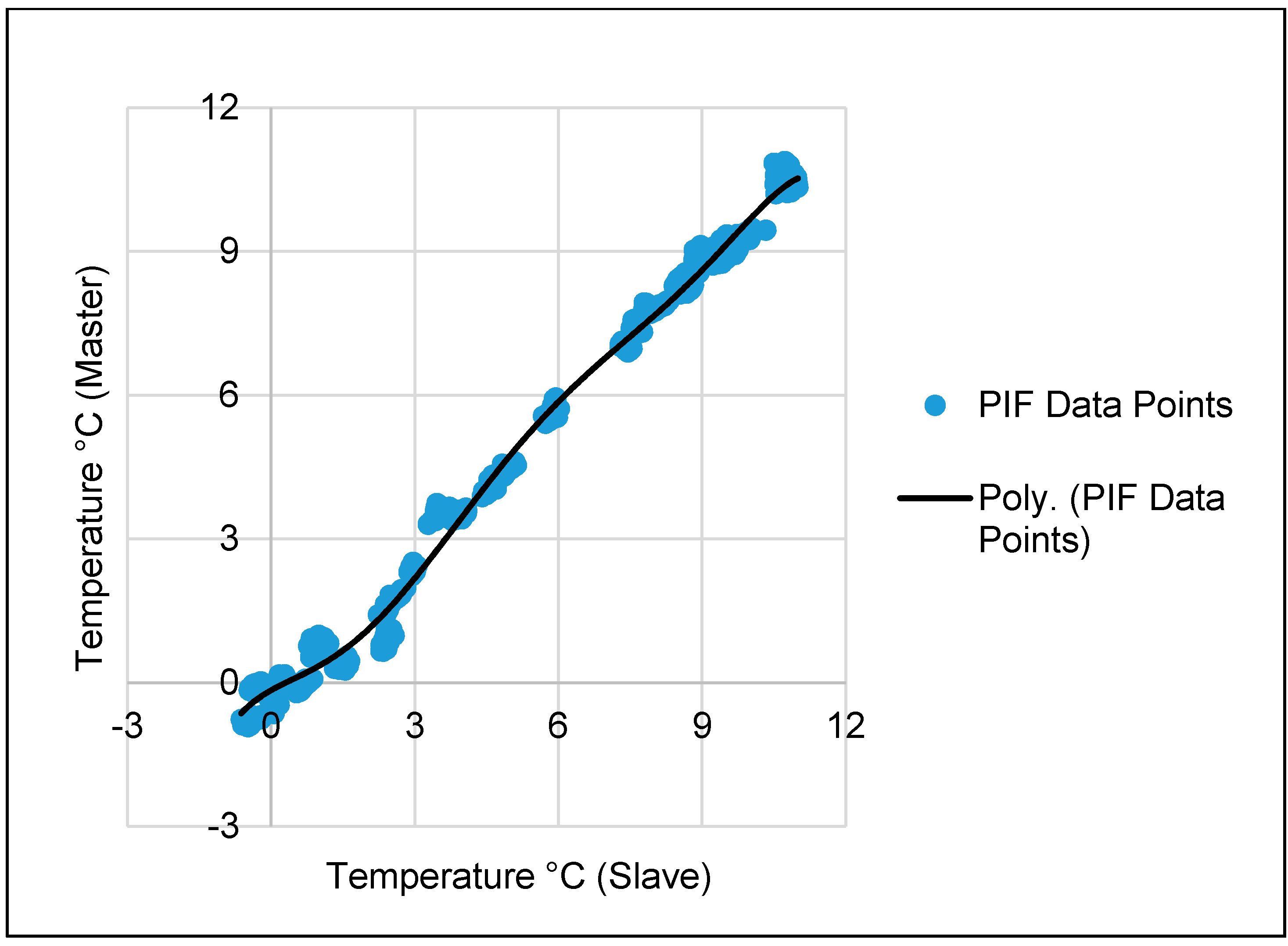
2.2.2. Pseudo-Invariant Feature (PIF)-Based Polynomial Regression (PIF_Poly)

Pseudo-invariant features (PIFs) are defined as objects whose electromagnetic properties (reflection, absorption and emission) are nearly constant during the imaging conditions and which are independent of seasonal or biological cycles [22]. Such features are commonly used as references for the relative radiometric normalization of multi-temporal imagery [6,13,22,23,24]. In this study, we used four types of PIFs that were expected to be consistent during the acquisition of both flight lines: (i) grass; (ii) roof top; (iii) river water; and (iv) road; each of which cover a broad (non-overlapping) range of temperatures. In general, grass and roofs were cooler than most of the features within each flight line; water was warmer and road was the hottest. We manually collected ~2000 training sample points (~500 points for each type of land cover) within the overlap sections. These points were then plotted (Figure 3) and a sixth order polynomial regression equation (Equation (2)) was developed from the scatterplot, which was later used to normalize the slave image to the master. We note that numerous orders of polynomial regression were evaluated before concluding that for these samples, a sixth order polynomial was optimal.
y = 0.0001 x 6 + 0.0033 x 5 0.0387 x 4 + 0.1796 x 3 0.2020 x 2 + 0.5659 x + 0.1583   ( R 2 = 0.99 )
Figure 3. A scatterplot of pseudo-invariant features (PIFs) selected within the overlap of the master and the slave images. These PIFs represent a combination of four land cover classes (grass, river water, rooftop and road) and are shown modeled with a sixth order polynomial trend line (black). Poly, polynomial.
Remotesensing 06 11810 g003

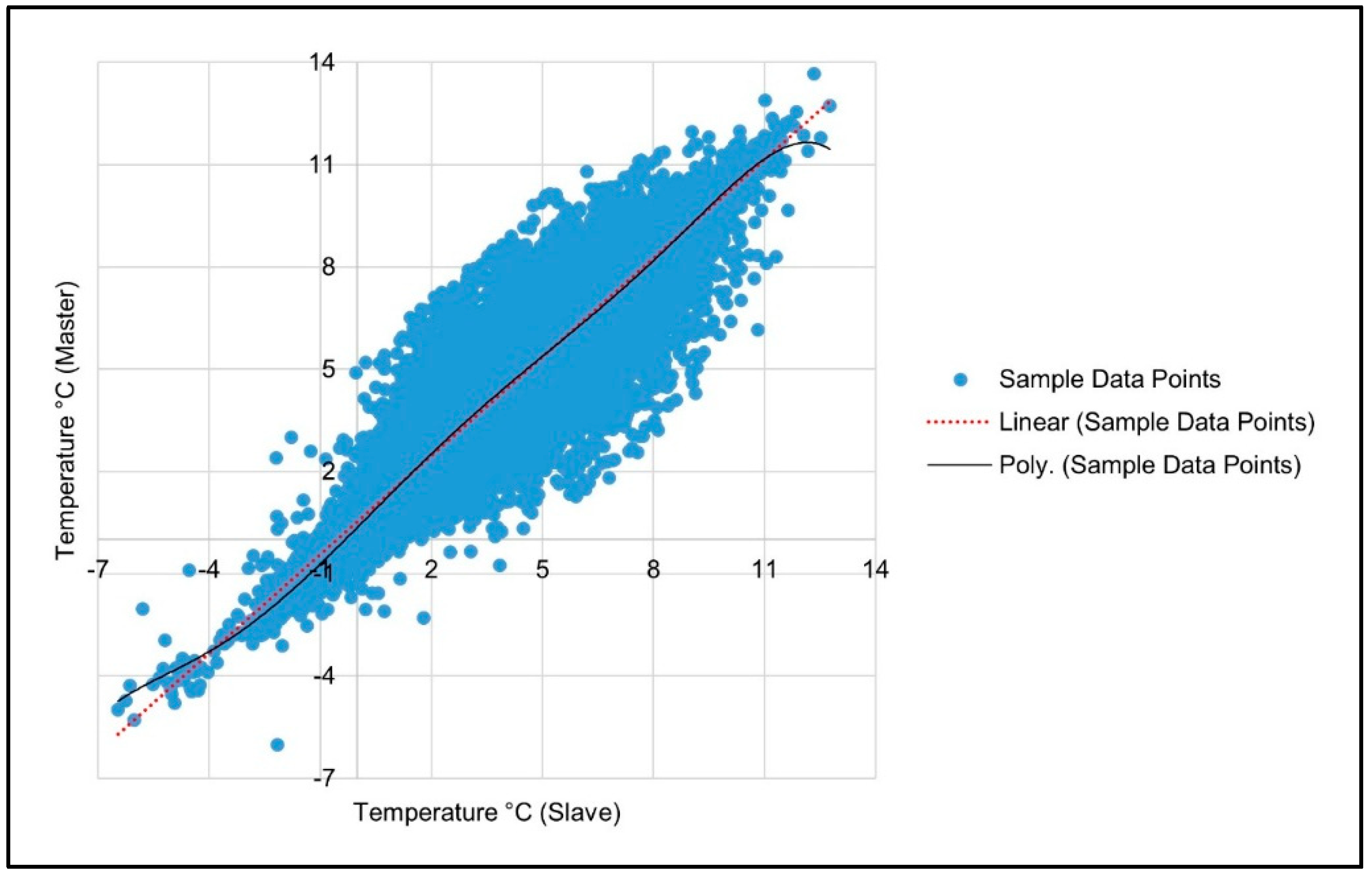
2.2.3. No-Change Stratified Random Sample (NCSRS)-Based Linear Regressions

The manual selection of PIFs is subject to user bias and errors and can be difficult, time consuming and costly to complete correctly, especially in areas where the analyst may have limited local field experience. To overcome these issues, a number of studies describe using automatic techniques to identify no-change sets (i.e., invariant features) from which they select reference samples for relative radiometric normalization [6,8,13,25,26,27]. In this paper, we apply the method described in Rahman et al. [13], which used the mean and standard deviation (SD) to automatically identify the no-change set within the flight line overlap. This required producing an image difference map of the overlap sections by subtracting the slave from the master overlap (i.e., Master DN-Slave DN), then creating a histogram from this difference map.
As these flight lines were collected during a calm night only ~20 min apart, we assumed that the temperature of different land cover types was not significantly altered. Consequently, any abrupt changes in surface temperature during this brief time are considered as noise and are masked out of the image difference histogram using a heuristically-derived measure of SD. Due to the airborne nature of these data, we note that this activity also compensates for areas within the scene that may have localized geometry issues greater than the reported geometric error (±1 m) of the post-processed data. “Compensates for” means that areas with large geometric error are expected to show high variance in the change image; thus, these areas are not included in the analysis. This SD measure corresponds to data points (i.e., DNs) beyond the mean ±3SD, which has been extensively shown to work over different cover types [13]. To collect representative samples from the remaining image, the master and slave overlap DN pairs were sorted in an ascending order, and a random pair was selected from each 500-point bin (i.e., 0.2% of the population); in this case, totaling 42,280 sample points. Data were sorted to cover the entire radiometric range of the overlap image, so that different land cover types (with different temperatures) are included in the samples. The selected samples were then plotted (Figure 4) to develop a linear regression equation (Equation (3)), which is then applied over the slave image to radiometrically normalize it to the master image.
y = 0.9124 x +   0.334   ( R 2 = 0.88 )
Figure 4. A scatterplot of no-change stratified random samples (NCSRS) with a sixth order polynomial trend line (black) and a linear trend line (red dotted) between the master and the slave images.
Remotesensing 06 11810 g004

2.2.4. No-Change Stratified Random Sample (NCSRS)-Based Polynomial Regression

The same samples (Figure 4) that are used for NCSRS-based linear regression (Section 2.2.3) are used here to develop a polynomial regression equation (Equation (4)). This equation is used to radiometrically normalize the slave image to the master.
y = 0.000004 x 6 0.00009 x 5 + 0.00017 x 4 +   0.00696 x 3 0.3294 x 2 + 0.95803 x 0.1189   ( R 2 = 0.93 )

2.3. Validation of the Results Using Root Mean Square Error (RMSE)

It is expected that the radiometric (temperature) difference between identical features in the master and the slave flight lines (within the overlap) will decrease after performing normalization. To test this, we randomly selected 2000 test points from the four major land cover types present in the overlap sections, including: (i) grass; (ii) rooftop; (iii) river water; and (iv) road (~500 points for each type of land cover); then, we calculated the root mean square error (RMSE) of the selected points for all presented methods using Equation (5).
R M S E = 1 n   ( D N m a s t e r     D N s l a v e ) 2 n
The RMSEs are then compared (see Section 3) to assess the performance of all methods. RMSE is used as an overall comparative measure of fitness, as it defines the difference between values predicted by the model and the observed values. The smaller the RMSE, the closer the model is to the observed values.

3. Results and Discussions

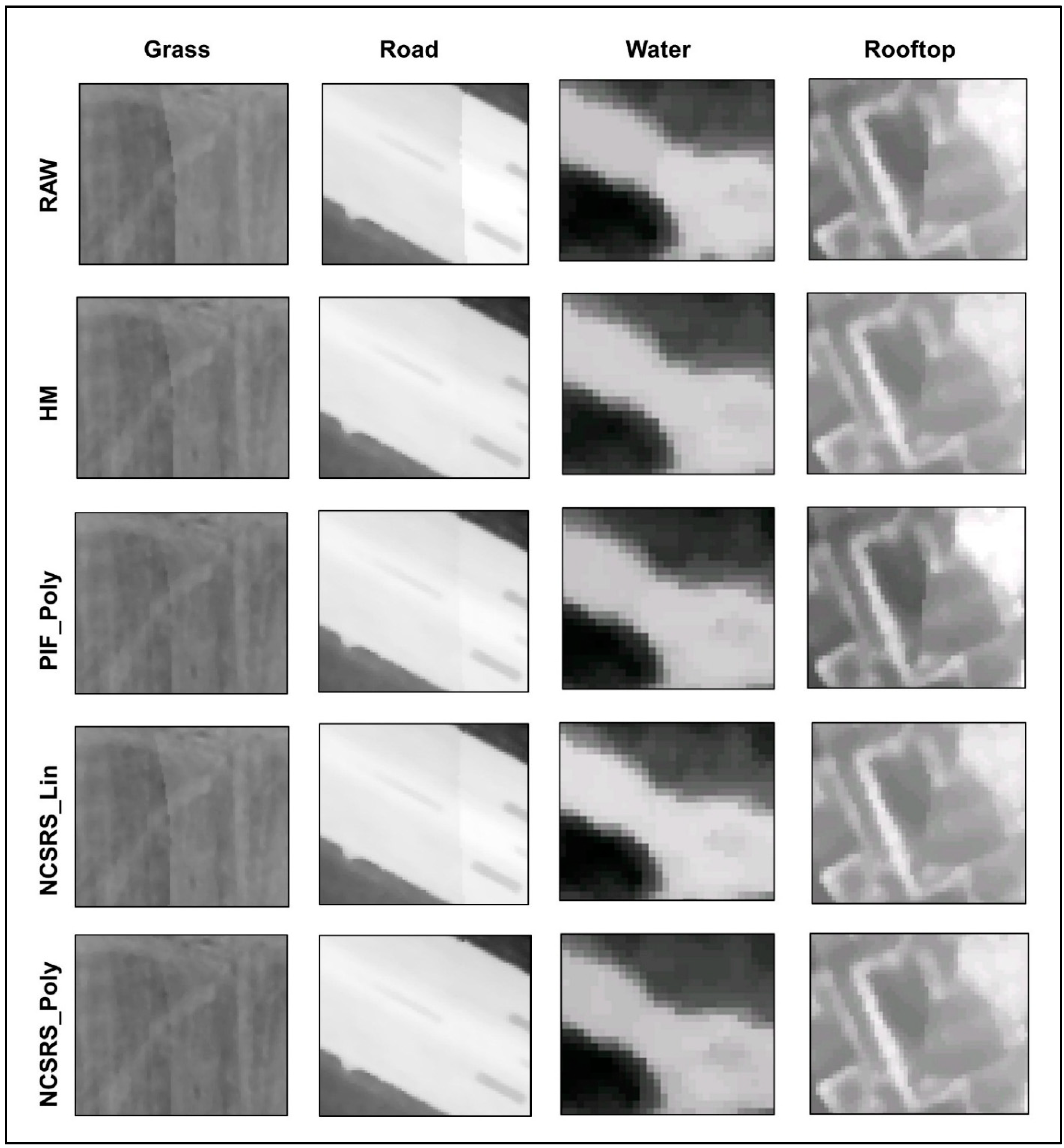
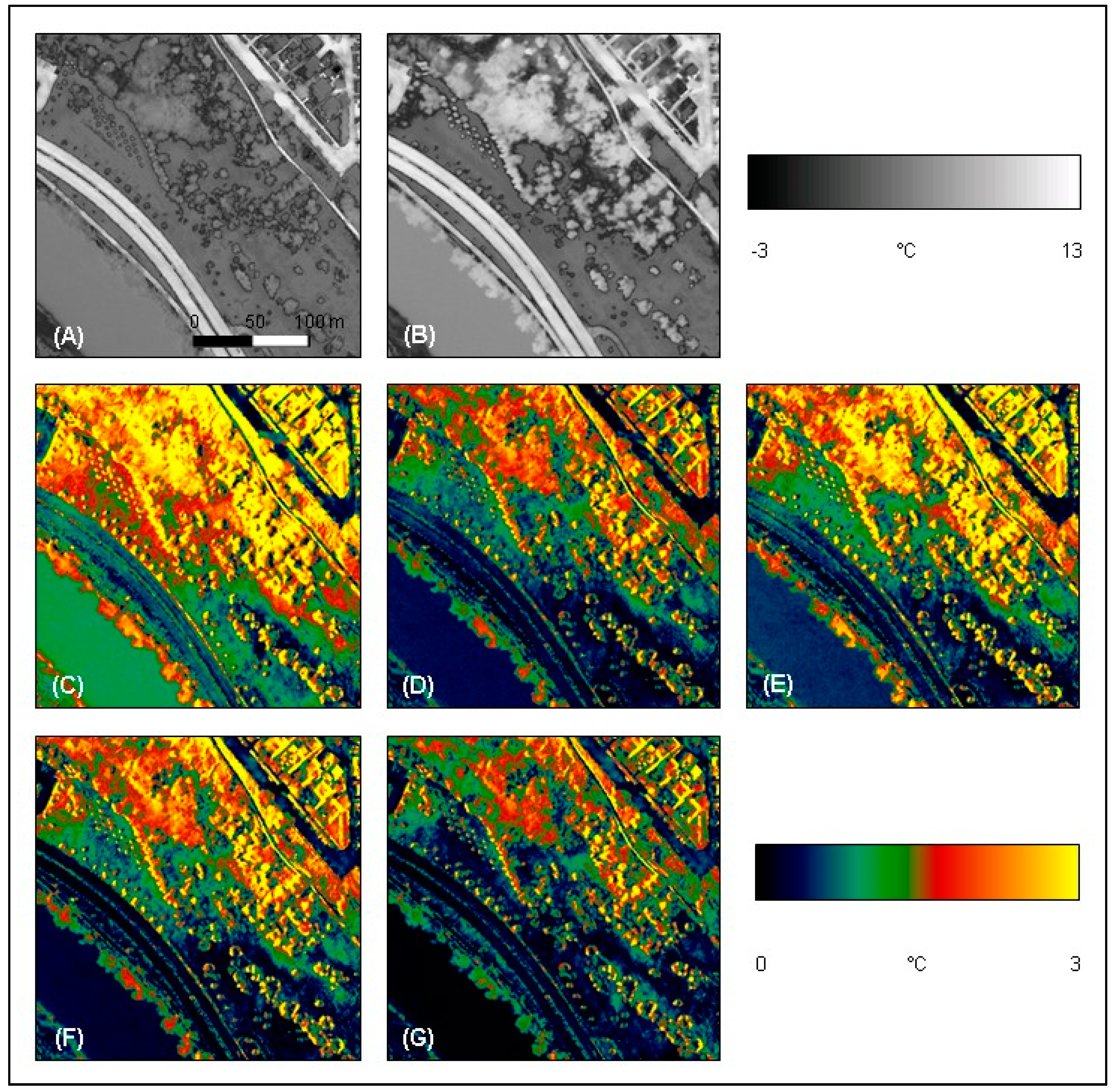
3.1. Visual Assessments

Visual assessment is a straightforward way to judge the performance of the evaluated methods. In so doing, the master and the slave flight lines were joined and features along the mosaic line were assessed. If the visual differences between the master and the normalized slave images are smaller than that of the master and the raw slave images, the normalized image can be considered as radiometrically fitted to the reference image.
A visual assessment of grass, road, water and rooftop samples (illustrated in Figure 5) shows that each tested method visually improves the radiometric agreement between the master and the slave images compared to the raw image. However, the degree of normalization varies depending on the method used and the land cover type assessed. Specifically:
HM appears to perform very well for road and water, but performs only moderately well for grass and rooftop.
PIF_Poly performs well for road and water and moderately well for grass, but it does not perform well for rooftop.
NCSRS_Lin performs very well for water and moderately well for road, grass and rooftop.
NCSRS_Poly performs very well for road and water and well for grass and rooftop. Though subjective, we further suggest that grass and rooftop visually appear best modeled by this method.
Figure 5. Visual examples of four different relative radiometric normalization methods applied along the mosaic join line of four different land cover types (grass, road, water and rooftop). PIF_Poly—pseudo-invariant feature-based polynomial regression; NCSRS_Lin-no-change stratified random sample-based linear regression.
Remotesensing 06 11810 g005
In general, the radiometric error of geographically simple features, like road and water, are visually reduced by all methods; this, in part, can be explained by their high thermal inertia, which results in low within-class variability (regardless of their acquisition time within either flight line).
We also note that while the river water class is a part of a dynamic system, its nighttime temperature fluctuates very little as its source is regulated by high mountain snow melt. However, complex features, like grass and rooftops, are not well modeled by most of the evaluated methods. This, in part, can be explained by their complex and variable nature. That is: (i) Different types of grass will exhibit different nighttime evapotranspiration rates; and (ii) the temperature of different roof sections (even for the same building structure) can be differentially heated at different times during the night, as they respond to varying local microclimatic differences in temperature and humidity—two attributes typically assessed by modern in-home thermostats. At a broader community scale, roof tops can further be considered a highly variable land cover feature, as they are composed of numerous materials, many of which have different emissivity characteristics that need to be corrected for (after radiometric normalization) in order to convert their relative temperature values (defined by the sensor) to true kinetic temperatures [2,3]. As a consequence, a small constant difference in (relative) ambient temperature may result in several degrees of difference in roofs composed of different materials, which are not corrected for emissivity.
Figure 6 provides another visual example of how the four evaluated relative radiometric normalization techniques reduce the thermal variability between the master and slave image(s) for four different land cover types. Figure 6A (the master) and 6B (the slave) represent corresponding grey-scale TABI-1800 image samples of a small area located within the flight line overlap that is predominantly composed of vegetation, roads, a (water-body) river and roofs. In both of these grey-scale sub-images, grass (smooth lower right) and roofs (top right corner) appear cool (mid-dark grey), the river (lower left diagonal feature) and trees (textured blobs) are moderately warm (light grey), while roads and paths are the hottest (white). In Figure 6C, the strongest temperature difference between the master and the uncorrected (raw) slave image appears yellow (+3 °C) for trees and rooftops. However after radiometric normalization, these differences and those of other features tend to visually decrease (Figure 6D–G). For example, water and road appear well modeled by most of the methods, displaying a minimum difference (i.e., black or blue ≈ 0–1 °C) between the master and the normalized slave images. Overall, rooftops and trees display the highest differences (yellow ≈ +3 °C), which perpetuates over different spatial extents in all slave images. Upon more detailed visual inspection, these yellow coloured rooftops and trees appears to be due to geometric shift-differences, especially noticeable as yellow regions along the edge of buildings (see the top right Figure 6D–G) and on tree-tops and along paths (within the same figures). However, based on a visual assessment of the pseudo-coloured temperature differences for all of the RRN samples, NCSRS_Poly visually appears to perform the best for all four land cover types (as it exhibits the most black and blue colors, thus representing the smallest temperature differences), closely followed by HM and NCSRS_Lin.
Figure 6. A visual example of how relative radiometric normalization techniques decrease the radiometric variability between flight lines. (A) A sample area from the master image. (B) The same area from the slave image. Pseudo-colored absolute image difference (C) between the master and the uncorrected slave image and between the master and the normalized salve images resulting from (D) HM, (E) PIF_Poly, (F) NCSRS_Lin and (G) NCSRS_Poly.
Remotesensing 06 11810 g006

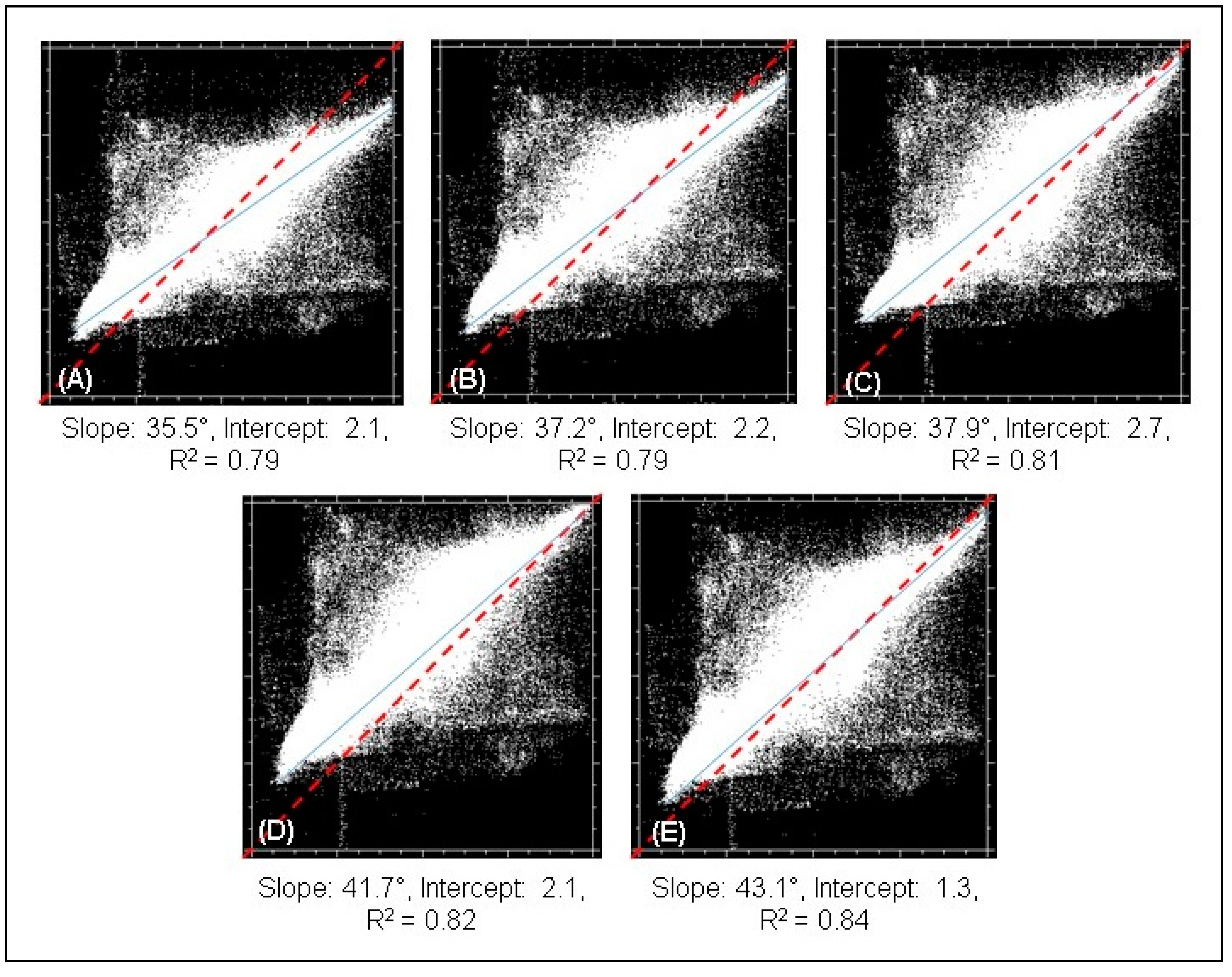
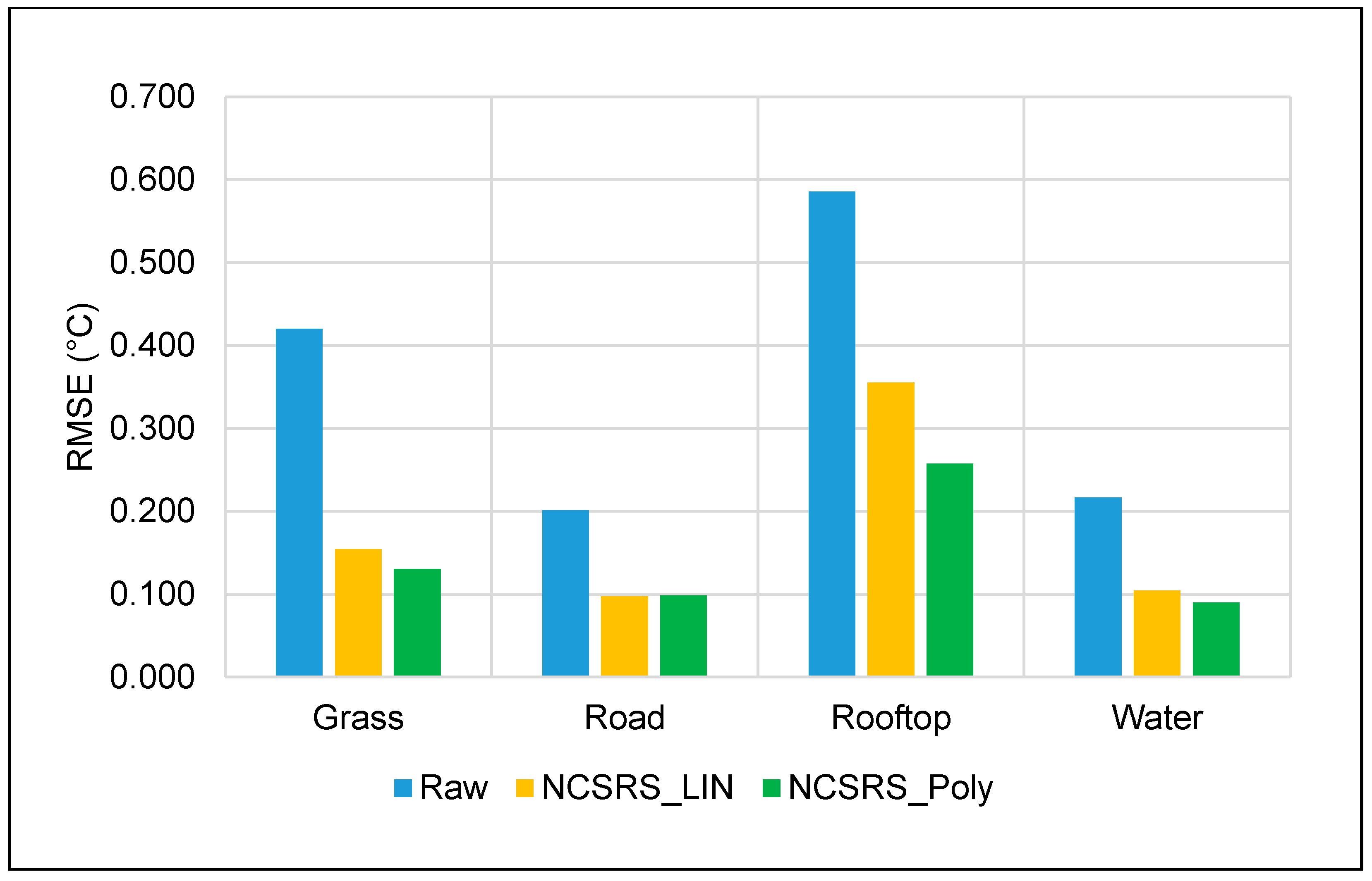
3.2. Statistical Analysis

As noted in Section 2.2.4, the root mean square error (RMSE) was used to define the statistical agreement between the normalized slave images and the master image. This required collecting 2000 stratified random sample points within the overlap that represent four different land cover types over a wide range of temperatures. These include: (i) grass; (ii) road; (iii) water; and (iv) rooftop. Table 1 summarizes the RMSEs calculated for these cover types.
Table 1. The overall RMSE of four different land cover types, for each of the four different relative radiometric normalization methods evaluated in this study. Bold values represent the lowest RMSE of each class and overall RMSE calculated for each image.
Land Cover TypeRMSE (°C)
SlaveHMPIF_PolyNCSRS_LinNCSRS_Poly
Grass0.4200.2360.2270.1930.163
Road0.2010.0970.1280.1220.123
Rooftop0.5860.4360.4520.3710.322
Water0.2160.1060.1080.1300.113
Overall *0.3560.1940.2100.1730.159
* Mean of RMSEs of all selected test samples for different land cover types.
In general, all methods show a reduced radiometric variation between the master and the slave images. From Table 1, we see that complex features, like rooftops and grass, have higher RMSE values in the uncorrected slave image than other features. This is understandable, as different roofing materials are used in Calgary, including asphalt shingles, clay tiles, cedar, tar and gravel, wood, concrete, fibreglass, vinyl shingles, etc. each of which have different thermal capacities, conductivity and emissivity. As a result, we found it challenging to radiometrically normalize rooftops with each of the methods. Similarly, the grass class also has a higher RMSE in the uncorrected slave image, potentially due to: (i) the various species compositions, each with varying allometric and morphometric characteristics; and (ii) the varying amount of moisture in the background soil [28]. The other two features (road and water) are relatively simple and exhibit relatively lower RMSE values in the slave image. They are also reasonably well modeled by all methods, resulting in decreased RMSE values (~50%). However, the complex feature classes (rooftop and grass) are best modeled only by the NCSRS-based methods, with the NCSRS-based polynomial technique providing the lowest overall RMSE values (0.322 and 0.163 respectively).
Figure 7 illustrates the scatterplots and resulting trend-lines between the master and the slave images before (Figure 7A) and after (Figure 7B–E) normalization. The blue lines represent the linear trend lines, while the red dashed lines illustrate the expected trend of each dataset at perfect radiometric agreement. Scatterplots can be used to describe various correlations between different variables. A high positive linear correlation exists between two datasets when the data cloud follows a 45° diagonal line (i.e., the red dotted line in Figure 7A–E). This indicates that the datasets are not only highly correlated, but also that their DN values are very close to each other.
In a perfect scenario, if two datasets represent the same features, their slope in the scatterplot should be 45° and their intercept should be at zero. In the scatterplot of the raw images (Figure 7A), the slope is shown to be 35.5° and the intercept is shown as 2.1. However, each of the normalized scatterplots (Figure 7B–E) improves the slope between the master and the slave, and most of the methods improve both the intercept and the slope. Of those methods tested, the scatterplot results (Figure 7A–E) show that the NCSRS_Poly trend line (Figure 7E) is visually and statistically the closest to the red line with a slope of 43.1°, an intercept of 1.3 and an R2 of 0.84. Thus, it represents the best performing normalization method, followed by NCSRS_Lin (Figure 7D). Conversely, while the HM method improves the slope between the master and the slave (indicating that the radiometric agreement is supposed to improve), the intercept is slightly increased, and in the case of PIF_Poly, the intercept is further increased (meaning that the radiometric agreement is supposed to be decreased).
Figure 7. (A) A comparison of the scatterplot between the original master and the slave images and after applying four normalization methods: (B) HM; (C) PIF_Poly; (D) NCSRS_Lin; and (E) NCSRS_Poly. The thin blue lines describe the data trend line, while the red dashed lines show the expected trend(s) at perfect radiometric agreement.
Remotesensing 06 11810 g007

3.2.1. A Comparison of Automatic vs Manual Methods

When automatic methods (HM, NCSRS_Lin and NCSRS_Poly) are compared against the manual method (PIF_Poly), the Table 1 results demonstrate that automated methods are able to more efficiently process large volumes of data, while maintaining a higher level of accuracy (i.e., a lower RMSE). Figure 5 and Table 1 further show that although the (PIF_Poly) method performed moderately well for grass, road and water, it failed to improve the radiometric agreement for rooftops. Additionally, the required manual collection of samples is time consuming, subject to human error and not easily operationalized for large datasets.

3.2.2. An Assessment of Computation Time

When analyzing large area, H-res TIR imagery, especially within an operational setting, computation time is an important criterion to consider. In order to meaningfully assess the computation times for each of the evaluated radiometric normalization methods, we applied each method over the same datasets and used the same workstation for subsequent analysis. All algorithms were written (in house) in the Interactive Data Language (IDL 8.0) and optimized for performance.
Processing results (Table 2) show that the NCSRS-based linear regression method required the least amount of time to execute (1.4 min). The second fastest method was histogram matching, which required 2.14 min; while NCSRS_Poly and PIF_Poly each took 4.7 min to compute. However we rate NCSRS_Poly as the third fastest, as its training samples were automatically selected. Conversely, PIF_Poly required the manual collection of training samples, which, in this case, took about 30 min to manually define (from within the overlap between the two flight lines). Furthermore, as the number of flight lines increases, this method becomes increasingly complicated, as additional samples will need to be manually collected from each overlap section. For example, if we were to use this method to process the full City of Calgary with its 43 TABI-1800 fight lines (~600 GB), we estimate 22 h of additional labour, just for manual sample collection (i.e., 42 overlaps × 30 min each). Thus, we rate PIF_Poly as the slowest method to implement and do not recommend it for large area operational analysis.
Table 2. Computation time of four different relative radiometric normalization (RRN) methods evaluated in this study.
RRN MethodComputing Time (min)
Histogram Matching2.14
PIF_Poly4.7 *
NCSRS_Lin1.4
NCSRS_Poly4.7
* Represents the computation time required after the manual collection of PIFs.

3.2.3. A Comparison of Linear vs Polynomial Methods

In the Introduction, we hypothesized that nonlinear (i.e., polynomial) RRN techniques are better suited to model the temperature variability of complex urban features in H-res TIR imagery than corresponding linear techniques. In this section, we test this hypothesis by comparing only the NCSRS-based linear and polynomial RRN techniques, as they both use the same automatically generated samples in their corresponding regression equations
From a visual assessment of the cover classes in Figure 5 and Figure 6 and the scatterplot agreement in Figure 7, we conclude that NCSRS_Poly visually performs better than NCSRS_Lin. Furthermore, Table 1 shows the lowest overall RMSE resulting from NCSRS_Poly. That is, when compared to the original slave test samples (Table 1), NCSRS_Poly decreases overall RMSE by 56%, which is 5% less than NCSRS_Lin (51%). However, if we only look at the results for the most complex class (rooftop), NCSRS_Poly decreases the RMSE by 46%, vs 36% for NCSRS_Lin.
From Figure 8, we see that results from the polynomial function (in green) display notable improvement over the raw data (blue) or the linear method (yellow) for the two complex land cover classes—grass and rooftop (each of which are characterized by greater internal variability). For more simple landscape features, like water and road, both methods perform very closely, with NCSRS_Poly only slightly better for water.
Figure 8. A comparison of linear (LIN) and polynomial (Poly) regression-based radiometric normalization using the same no-change stratified random samples (NCSRS).
Remotesensing 06 11810 g008
Based on this combination of results, it is clear that the polynomial technique (NCSRS_Poly) provides improved radiometric agreement over the linear technique, though we note that NCSRS_LIN is three-times faster to implement (see Table 2). Scaled for 43 flight lines, this represents a processing time of 58.8 min vs 197.4 min. While a faster implementation time is best, we consider NCSRS_Poly as the most operationally capable, based on the strength of its visual and statistical results, even with its (currently) slower implementation time. If necessary, increased processing speed can be gained from faster hardware.

4. Conclusions

This paper has evaluated two linear relative radiometric normalization techniques, (i) histogram matching and (ii) no-change stratified random sample-based linear regression, against two new polynomial RRN techniques, (iii) Pseudo invariant feature-based polynomial regression and (iv) no-change stratified random sample-based polynomial regression. One of the evaluated techniques required manual sample collection, while the other three were automatic.
Pseudo invariant feature-based polynomial regression (PIF_Poly) is based on a polynomial regression equation derived from a scatterplot formed by manually-selected pseudo-invariant feature point pairs (i.e., of grass, road, rooftop and water) extracted from the overlap between the master and the slave flight lines. Results show that this method is unsuitable for the operational radiometric normalization of H-res thermal infrared imagery in terms of time, visual assessment and statistical analysis. Specifically, it showed the highest overall RMSE for all classes; thus, it is the least accurate of those tested. Additionally, the manual selection of its reference points is time consuming and subject to human error, and as data volumes increase, the time and complexity of such a method will also increase.
Histogram matching (HM) performs a scalar shifting of the slave histogram to the reference histogram. This method is easy to understand, simple to implement, the second fastest of those tested and produces acceptable visual results. However, while a simple scalar adjustment is very good for relatively invariant features, like water or road, it does not work well for complex urban features, like rooftops and vegetation, which are present in all flight lines. Nevertheless, this method does not reduce the radiometric agreement. Overall, it produced the third highest RMSE for all classes. Thus, for a quick assessment with acceptable results, we still consider this method as effective.
No-change stratified random sample-based linear regression (NCSRS_Lin) generates a linear regression equation based on automatically selected sample points from the reference and the slave flight line overlaps. This linear regression method is computationally the fastest tested method; it is simple to understand, easy to execute and produces visually and statistically better results than HM, including those for complex features, like grass and rooftops.
No-change stratified random sample-based polynomial regression (NCSRS_Poly) generates a polynomial regression equation based on the same automatically generated sample set as NCSRS-based linear regression. In terms of computational time, this method is slower than HM and NCSRS-based linear regression; however, it achieved the best results from both visual and statistical assessments. We ranked it third fastest in computation time, tying with (PIF_Poly), but beating it, due to its automatic sampling feature. In particular, the non-linear characteristic of this method, when applied to a large number of automatically collected samples, was the best at modelling complex urban surfaces, especially urban rooftops and grass. It also performed well for less complex features, such as road and water.
In summary, all four of the methods evaluated in this paper have increased the radiometric agreement between the reference and the slave image. In terms of time, NCSRS-based linear regression was the fastest method, and it also generated visually and statistically acceptable results. In terms of statistical results, the NCSRS-based polynomial regression method produced the best results, with its radiometric agreement (between the master and the slave image) increasing by ~56%, closely followed by NCSRS-based linear regression (~51%). Results show that the non-linear method (NCSRS_Poly) better models the various heterogeneous thermal properties of a complex urban landscape compared to the evaluated linear methods; thus, we recommend it as the most appropriate to use for normalizing H-res airborne TIR urban imagery.

Acknowledgments

We acknowledge support from The Institute for Sustainable Energy, Environment and Economy (ISEEE) (www.iseee.ca), ITRES Research Limited (www.itres.com), The City of Calgary (www.calgary.ca), Tecterra (www.tecterra.com), NSERC (www.nserc.ca), The Alberta Real Estate Foundation (www.aref.ab.ca) and the Calgary Real Estate Board (www.creb.com). We also acknowledge a University of Calgary Faculty Graduate Research Scholarship and a Geography Excellence Award provided to Mir Mustafizur Rahman and an Alberta Informatics Circle of Research Excellence (iCore) Scholarship and an ISEEE Graduate Scholarship awarded to Bharanidharan Hemachandran.

Author Contributions

Mir Mustafizur Rahman processed the thermal data, analyzed the results, wrote the paper, and is the main author of the article. Geoffrey J. Hay helped with ideas and technical advices during the development stage of the algorithm and also contributed in reviewing the paper. Isabelle Couloigner and Bharanidharan Hemachandran helped in editing the paper, and Jeremy Bailin contributed in developing IDL codes and in reviewing the paper.

Conflicts of Interest

The authors declare no conflict of interest.

References

  1. Voogt, J.A.; Oke, T.R. Complete urban surface temperatures. J. Appl. Meteorol. 1997, 36, 1117–1132. [Google Scholar] [CrossRef]
  2. Rahman, M.M.; Hay, G.J.; Couloigner, I.; Hemachandran, B.; Tam, A. Geographic object-based mosaicing (OBM) of high-resolution thermal airborne imagery (TABI-1800) to improve the interpretation of urban image objects. IEEE Geosci. Remote Sens. Lett. 2013, 10, 918–922. [Google Scholar] [CrossRef]
  3. Rahman, M.M.; Hay, G.J.; Couloigner, I.; Hemachandran, B. Transforming image-objects into multiscale fields: A GEOBIA approach to mitigate urban microclimatic variability within H-Res thermal infrared airborne flight lines. Remote Sens. 2014, 6, 9435–9457. [Google Scholar] [CrossRef]
  4. Hill, J.; Sturm, B. Radiometric correction of multitemporal thematic mapper data for use in agricultural land-cover classification and vegetation monitoring. Int. J. Remote Sens. 1991, 12, 1471–1491. [Google Scholar] [CrossRef]
  5. Du, Y.; Teillet, P.M.; Cihlar, J. Radiometric normalization of multitemporal high-resolution satellite images with quality control for landcover change detection. Remote Sens. Environ. 2002, 82, 123–134. [Google Scholar] [CrossRef]
  6. Hall, F.G; Sterbel, D.E.; Nickeson, J.E.; Goetz, S.J. Radiometric rectification: Toward a common radiometric response among multidate, multisensory images. Remote Sens. Environ. 1991, 35, 11–27. [Google Scholar] [CrossRef]
  7. Chen, X.; Vierling, L.; Deering, D. A simple and effective radiometric correction method to improve landscape change detection across sensors and across time. Remote Sens. Environ. 2005, 98, 63–79. [Google Scholar] [CrossRef]
  8. Canty, M.J.; Nielsen, A.A.; Schmidt, M. Automatic radiometric normalization of multitemporal satellite imagery. Remote Sens. Environ. 2004, 91, 441–451. [Google Scholar] [CrossRef]
  9. Fernandes, R.; Leblance, S.G. Parametric (modified least squares) and non-parametric (Theil-Sen) linear regressions for predicting biophysical parameters in the presence of measurement errors. Remote Sens. Environ. 2005, 95, 303–316. [Google Scholar] [CrossRef]
  10. Xing, Y.; Jiang, Q.G.; Qiao, Z.P.; Li, W.Q. Study of relative radiometric normalization based on multitemporal ASTER images. Adv. Mater. Res. 2010, 108, 190–194. [Google Scholar] [CrossRef]
  11. Warner, T.A.; Chen, X. Normalization of Landsat thermal imagery for the effects of solar heating and topography. Int. J. Remote Sens. 2001, 22, 773–788. [Google Scholar] [CrossRef]
  12. Scheidt, S.; Ramsey, M.; Lancaster, N. Radiometric normalization and image mosaic generation of ASTER thermal infrared data: An application to extensive sand sheets and dune fields. Remote Sens. Environ. 2003, 112, 920–933. [Google Scholar] [CrossRef]
  13. Rahman, M.M; Hay, G.J.; Couloigner, I.; Hemachandran, B.; Bailin, J.A. A comparison of four radiometric normalization techniques for mosaicing H-res multi-temporal thermal infrared flight lines of a complex urban scene. ISPRSJ. Photogramm. Remote Sens. 2014. accepted. [Google Scholar]
  14. Theil, H.A. Rank-Invariant Method of Linear and Polynomial Regression Analysis. Available online: http://link.springer.com/chapter/10.1007/978-94-011-2546-8_20 (accessed on 10 September 2014).
  15. Sen, P.K. Estimates of the regression coefficient based on Kendall’s Tau. J. Am. Stat. Assoc. 1968, 63, 1379–1389. [Google Scholar] [CrossRef]
  16. Peng, H.; Wang, S.; Wang, X. Consistency and asymptotic distribution of the Theil-Sen estimator. J. Stat. Plan. Infer. 2008, 138, 1836–1850. [Google Scholar] [CrossRef]
  17. Kahle, A.B.; Gillespie, A.R.; Goetz, A.F. Thermal inertia imaging: A new geologic mapping tool. Geophys. Res. Lett. 1976, 3, 26–28. [Google Scholar] [CrossRef]
  18. Jensen, J.R. Remote Sensing of the Environment: An Earth Resource Perspective, 2nd ed; Pearson Prentice Hall: Upper Saddle River, NJ, USA, 2007. [Google Scholar]
  19. Oke, T.R. Canyon geometry and the nocturnal urban heat island: Comparison of scale model and field observations. J. Climatol. 1981, 1, 237–254. [Google Scholar] [CrossRef]
  20. Chudnovsky, A.; Ben-Dor, E.; Saaroni, H. Diurnal thermal behavior of selected urban objects using remote sensing measurements. Energ. Build. 2004, 36, 1063–1074. [Google Scholar] [CrossRef]
  21. Richards, J.A. Remote Sensing Digital Image Analysis; Springer: NewYork, NY, USA, 1999. [Google Scholar]
  22. Schott, J.R.; Salvaggio, C.; Vochok, W.J. Radiometric scene normalization using pseudo-invariant features. Remote Sens. Environ. 1988, 26, 1–16. [Google Scholar] [CrossRef]
  23. Salvaggio, C. Radiometric scene normalization utilizing statistically invariant features. In Proceedings of Workshop Atmospheric Correction of Landsat Imagery, Torrance, CA, USA, 29 June–1 July 1993.
  24. Bao, N.; Lechner, A.M.; Fletcher, A.; Mellor, A.; Mulligan, D.; Bai, Z. Comparison of relative radiometric normalization methods using pseudo-invariant features for change detection studies in rural and urban landscapes. J. Appl. Remote Sens. 2012, 6. [Google Scholar] [CrossRef]
  25. Elvidge, C.D.; Yuan, D.; Ridgeway, D.W.; Lunetta, R.S. Relative radiometric normalization of Landsat Multispectral Scanner (MSS) data using an automatic scattergram-controlled regression. Photogmm. Eng. Remote Sens. 1995, 61, 1255–1260. [Google Scholar]
  26. de Carvalho, O.A.; Júnior; Guimarães, R.F.; Silva, N.C.; Gillespie, A.R.; Gomes, R.A.T.; Silva, C.R.; de Carvalho, A.P.F. Radiometric normalization of temporal images combining automatic detection of pseudo-invariant features from the distance and similarity spectral measures, density scatterplot analysis, and robust regression. Remote Sens. 2013, 5, 2763–2794. [Google Scholar] [CrossRef]
  27. Hu, C.M.; Ping, T. Automatic algorithm for relative radiometric normalization of data obtained from Landsat TM and HJ-1A/B charge-coupled device sensors. J. Appl. Remote Sens. 2012, 6. [Google Scholar] [CrossRef]
  28. Friedl, M.A.; Davis, F.W. Sources of variation in radiometric surface temperature over a tallgrass prairie. Remote Sens. Environ. 1994, 48, 1–17. [Google Scholar] [CrossRef]

