Article

Cultivated Land Information Extraction and Gradient Analysis for a North-South Transect in Northeast Asia between 2000 and 2010

1
State Key Laboratory of Resources and Environmental Information System, Institute of Geographic Sciences and Natural Resources Research, Chinese Academy of Sciences, Beijing 100101, China
2
Sichuan Province in second Geographic Information Engineering Institute of Surveying and Mapping, Chengdu 610031, China
3
College of Agriculture and Biotechnology, China Agricultural University, Beijing 100094, China
4
University of Chinese Academy of Sciences, Beijing 100049, China
5
Jiangsu Center for Collaborative Innovation in Geographical Information Resource Development and Application, Nanjing 210023, China
*
Author to whom correspondence should be addressed.
Remote Sens. 2014, 6(12), 11708-11730; https://doi.org/10.3390/rs61211708
Submission received: 12 June 2014 / Revised: 17 November 2014 / Accepted: 18 November 2014 / Published: 25 November 2014

Abstract

:
Cultivated land resources are an important basis of regional sustainability; thus, it is important to determine the distribution of the cultivated land in the Northeast Asia trans-boundary area of China, Russia and Mongolia, which has a continuous geographic and ecological environment and an uneven population distribution. Extracting information about the cultivated land and determining the spatial and temporal distribution of its features in this large trans-boundary area is a challenge. In this study, we derived information about the cultivated land of the North-South Transect in Northeast Asia by Linear Spectral Mixing Model, using time series data with MODerate resolution Imaging Spectroradiometer (MODIS) in 2000 and 2010. The validation showed more than 98% pixels with a root mean square error less than 0.05. The overall accuracy and spatial consistency coefficients were 81.63% and 0.78 in 2000 and 72.81% and 0.75 in 2010, respectively. The transect analyses indicate the presence of a greater amount of cultivated land in the south and less in the north. China owns most of the cultivated land in the transect area, followed by Mongolia and then Russia. A gradient analysis revealed a decrease of 34.16% of the cultivated land between 2000 and 2010. The amount of cultivated land decreased 22.37%, 58.93%, and 64.73% in China, Russia, and Mongolia, respectively. An analysis shows that the amount of cultivated land is primarily influenced by the various land development and protection policies in the different counties in this trans-boundary area.

Graphical Abstract

1. Introduction

The trans-boundary area of China, Russia, and Mongolia in northeast Asia has varying ecosystems, diverse climate zones, and significantly differing human-land relationships. The region has a large population that is unevenly distributed [1,2,3]. Cultivated land is the most important agricultural resource supporting the people living in the region. Due to its vulnerability to both natural and human forces, the distribution of the cultivated land in the area is very sensitive to both regional and global climate changes as well as to changes in the human activity in the three countries, such as changes in agriculture policy and population. It is notable that the social and economic systems of Russia and Mongolia were reformed in the early 1990s, which has had an influence on the first 10 years of the 21st century. Thus, obtaining information on the distribution of the cultivated land and the recent dynamics in the region is significant for ecologically safe construction, regional sustainable development and long-term international cooperation.
Remote sensing technology has been widely applied to extract information about cultivated land. The methods can be divided into three categories: computer automatic extraction, visual interpretation and man-machine interactive interpretation. Computer automatic extraction algorithms include decision tree models, artificial neural networks, support vector machines models, etc. Deng [4], Stern [5] and Li [6] used decision tree models to extract cultivated land information. Hou [7], Wang [8], Bai [9] and Bruzzone [10] extracted built-up land information using an artificial neural network algorithm, with higher accuracy. Liu [11] constructed an elaborate crop classification system using a support vector machine. Combining the spectral and spatial texture features, Yao [12], Zhu [13], Peña-Barragán [14] and Vintrou [15] extracted highly accurate cultivated land information using an object-oriented approach. Ashraf M. [16] used a maximum likelihood supervised classification technique to extract cropland information from satellite data. Yan [17] and Liu [18] extracted relevant farmland information with a visual interpretation method using QuickBird, SPOT data and feature interpretation signs. Dou [19] and Zhao [20] extracted cultivated land information with an accuracy up to 98.22% using a man-machine interactive interpretation method, but this was both costly and time-consuming.
Each of the cultivated land extraction methods has various applications and limitations. First, the high and medium spatial resolution data were used primarily for cultivated land information extraction in small areas. Second, most of these remotely sensed data were selected in a specific time period (e.g., one day or a few days in a year) when users are conducting a cultivated land distribution study in specific regions, which can easily result in the loss of cultivated land information for land that is seasonally cultivated or abandoned for a period of time. For example, if the crops are cultivated in the autumn or winter, and the remotely sensed images are obtained in the summer, the extracted information may not include the land cultivated in the subsequent seasons.
Because of these challenges, MODerate resolution Imaging Spectroradiometer (MODIS) data were chosen for this study. These data have the advantages of a medium spatial resolution, daily coverage, high sensitivity, and cost-free distribution [21]. MODIS sensors have collected more than ten years of data on the earth’s surface and provide an excellent opportunity to extract and analyze the long-term spatiotemporal changes in cultivated land. A Linear Spectral Mixture Model (LSMM) method integrated with time series data was used to extract the cultivated land in this area. This method avoids the loss of daily images and information on seasonal or abandoned land. A transect approach was used to obtain the baseline of the cultivated land information for the long-term research in this area. Section 2 introduces the materials and related methodology. Section 3 presents the interpretation results of the transect in 2000 and 2010. Section 4 discusses the cultivated land’s spatial distribution, gradient change characteristics and the driving forces for these changes. A summary is presented in Section 5.

2. Materials and Methodology

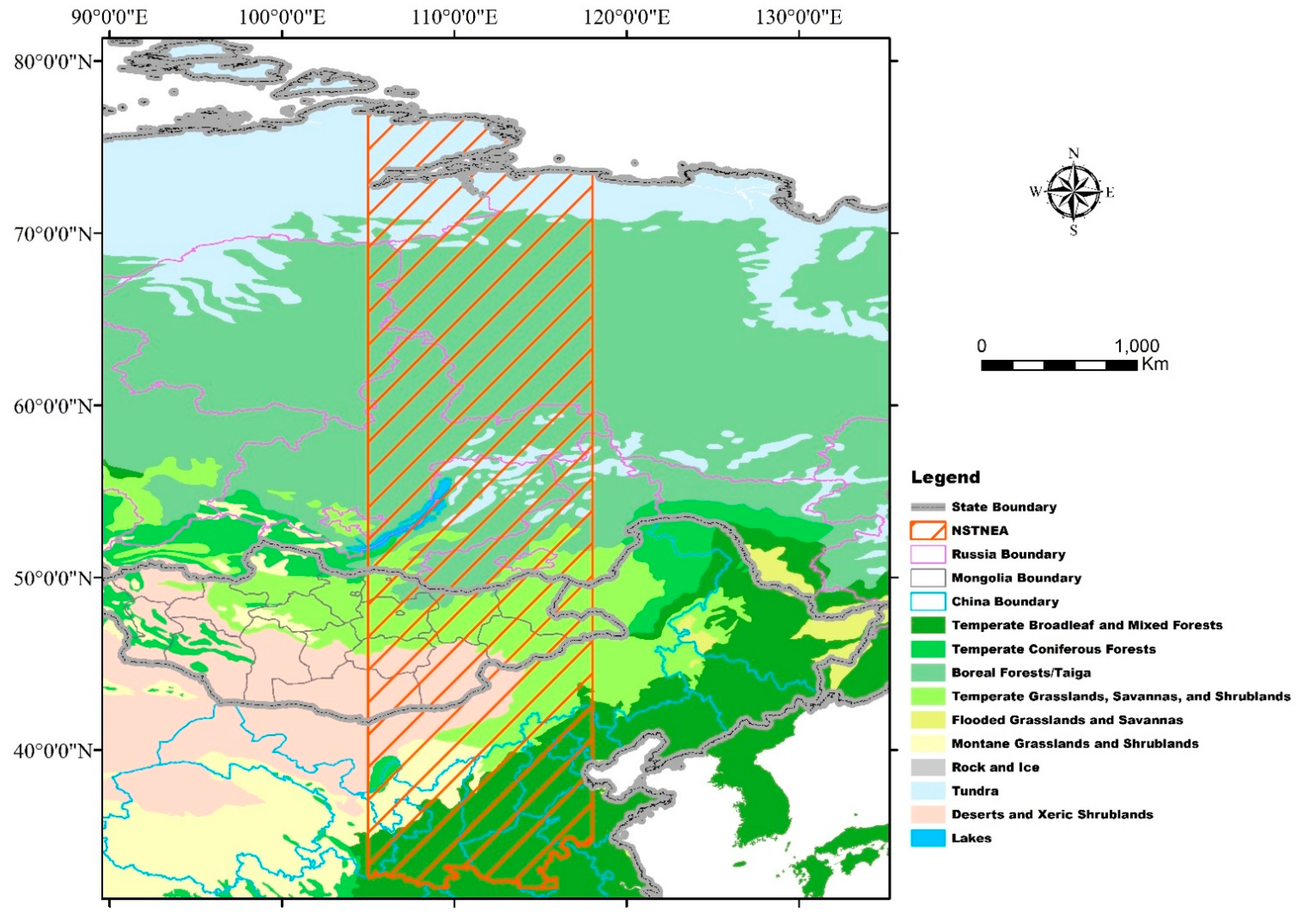
2.1. Study Area and Data

2.1.1. Study Area

A transect, which consists of a series of research sites and a global change driving gradient (temperature, precipitation, land use intensity, etc.), is a ribbon study area. It is considered to be one of the most effective methods of exploring the relationship between global change and terrestrial ecosystems [22]. The North-South Transect in Northeast Asia (NSTNEA) was selected as the study area because of its usefulness for discovering the cultivated land distribution characteristics of the larger area.
The NSTNEA was defined by Chinese, Russian and Mongolian scientists in 2008 [23]. It ranges from 32 to 78°N and 105 to 118°E. The transect centers on Lake Baikal, extending southward to the north bank of the Yellow River in China and northward to the polar region (Figure 1). The vegetation types along the transect vary gradually from broad-leaf forests, crops, and steppes in the south to conifer-deciduous broad-leaf mixed forests, conifer forests, boreal forests, and tundra in the north. This transect covers multiple eco-geographical zones from the south to north, i.e., mixed forest in the Loess Plateau, mixed forest in the Yellow River plain, deciduous forest in northeast China, East Siberian taiga, Baikal region coniferous forests, Dauria forest-steppe, Mongolian steppe, Selenge-Orkhon forest-steppe, southern Siberia forest-grasslands, Ordos Plateau grassland and Trans-Baikal bald mountain tundra biome [23]. The elevation ranges from 70 to 1400 m. The temperature and precipitation decrease with increase in the latitude. According to 2008 statistics, the average population density was 56 people per square kilometer. The highest density value was 39,171 people per square kilometer in Tianjin, China, and the lowest density value was less than 1 person per square kilometer in the northern area over latitude 68°N in Russia.
Figure 1. Location of the study area.
Remotesensing 06 11708 g001
By the end of 1991, a radical economic change had been implemented in the former Soviet Union, aimed at promoting the country’s economic transformation from a centrally planned economy to a market economy [24,25]. Mongolia launched a similar radical market-oriented reform in the early 1990s [26,27]. These reforms resulted in the economic decline of both countries during the transition until 2000.

2.1.2. Data

The data used in this study include the MODIS/Terra Vegetation Indices products, Digital Elevation Model (DEM) data, and cultivated land extraction accuracy evaluation data.
The MODIS/Terra Vegetation Indices (MOD13Q1) is a level 3 land data product with 250-m spatial resolution and 16-daytime resolution and includes 12 data sets (Table 1). The Normalized Differential Vegetation Index (NDVI) and Enhanced Vegetation Index (EVI) are important surface vegetation feature parameters that can indicate objective land cover characteristics. Because the EVI has a more enhanced vegetation detection capacity than the NDVI [28], it was selected as the basic data set for the cultivated land extraction in this study. The MOD13Q1 data for the year 2000 and 2010 were downloaded from the National Aeronautics and Space Administration’s (NASA) website [29]. Only images that were cloud-free and non-strip were selected and downloaded after careful quality control. A total of 345 images, including 18 temporal serials from the year 2000 and 300 images that included 16 temporal serials from the year 2010, were selected (Table 2). Two temporal serials from 2010 were omitted because of large areas without data in the images.
Table 1. MOD13Q1 data sets.
Data Sets NameBrief Description
250m_16_days_NDVINormalized Difference Vegetation Index
250m_16_days_EVIEnhanced Vegetation Index
250m_16_days_VI_QualityVegetation Index Quality
250m_16_days_red_reflectanceRed Reflectance
250m_16_days_NIR_reflectanceNIR Reflectance
250m_16_days_blue_reflectanceBlue Reflectance
250m_16_days_MIR_reflectanceMIR Reflectance
250m_16_days_view_zenith_angleView Zenith Angle
250m_16_days_sun_zenith_angleSun Zenith Angle
250m_16_days_relative_azimuth_angleRelative Zenith Angle
250m_16_days_composite_day_of_the_yearComposite Day of the Year
250m_16_days_pixel_reliabilityPixel Reliability Summary Quality
Table 2. EVI temporal series in 2000 and 2010 (format of the days: yyyyddd).
Day in 2000Day in 2010Temporal Serial
20000492010049T1
20000652010065T2
20000812010081T3
20000972010097T4
20001132010113T5
20001292010129T6
20001452010145T7
20001612010161T8
20001772010177T9
20001932010193T10
20002092010209T11
20002252010225T12
20002412010241T13
20002572010257T14
20002732010273T15
20002892010289T16
2010305----------T17
2010321----------T18
The selected images were mosaicked together by using the MODIS Reprojection Tool (MRT) [30]; the EVI data set was then extracted by using the ENVI software according to the boundary of the study area; finally, all of the pre-processed EVI data were stacked into a unified file for cultivated land extraction.
DEM data were used as auxiliary data. The Global 30 Arc-Second Elevation Data Set (GTOPO30) [31] was downloaded from the United States Geological Survey.
High-resolution land cover map data are required for accurate cultivated land assessment. However, only global level land cover data products that covered the entire transect area were available, and openly regional level data products were lacking. Because we selected the MODIS data sets as the input data sources for the cultivated land extraction, we didn’t select its land cover product as the reference data for the assessment of accuracy. The GLC2000 and GlobCover data sets were used in the study. The global land cover maps for the year 2000 (GLC2000) [32] and for the year 2009 (GlobCover2009) [33] were downloaded and used as global scale validation data. The GLC2000 was developed by the European Union’s Joint Research Centre. It was first developed regionally using experts in the field and then integrated into a single global product with the coarsest resolution at 1 km [34]. The overall accuracy of the GLC2000 is 68.6% (±5%) [35]. The GlobCover2009 was developed by the GlobCover consortium. A supervised and unsupervised classification algorithm was used to classify pixels with resolutions higher than 300 m. The overall accuracy of the GlobCover2009 is 67.5% [36,37].
The National Land-Use/Land-Cover Data-2000 of China (NLCD-2000) was used to validate the data in China. The NLCD-2000 was produced by approximately 100 scientists from eight research institutions in the Chinese Academy of Sciences using visual interpretation and digital image processing technology [38]. The production team made continuous efforts to provide updated land-use maps of the NLCD. To date, this dataset covers the periods of the late 1980s, 1995, 2000, 2005 and 2010. The land-use maps at a scale of 1:100,000 are drawn based on Landsat TM data, which has six first level classes and 25 second level classes. The average interpretation accuracy of the NLCD-2000 for land-use has been verified as 92.9% [39,40,41].
All of the land cover validation data were cut out by the boundary of the NSTNEA using the ENVI software. For the direct evaluation of the accuracy of the cultivated land information, all of the land cover validation data were reclassified into one of two classes: cultivated land or non-cultivated land.

2.2. Methodology

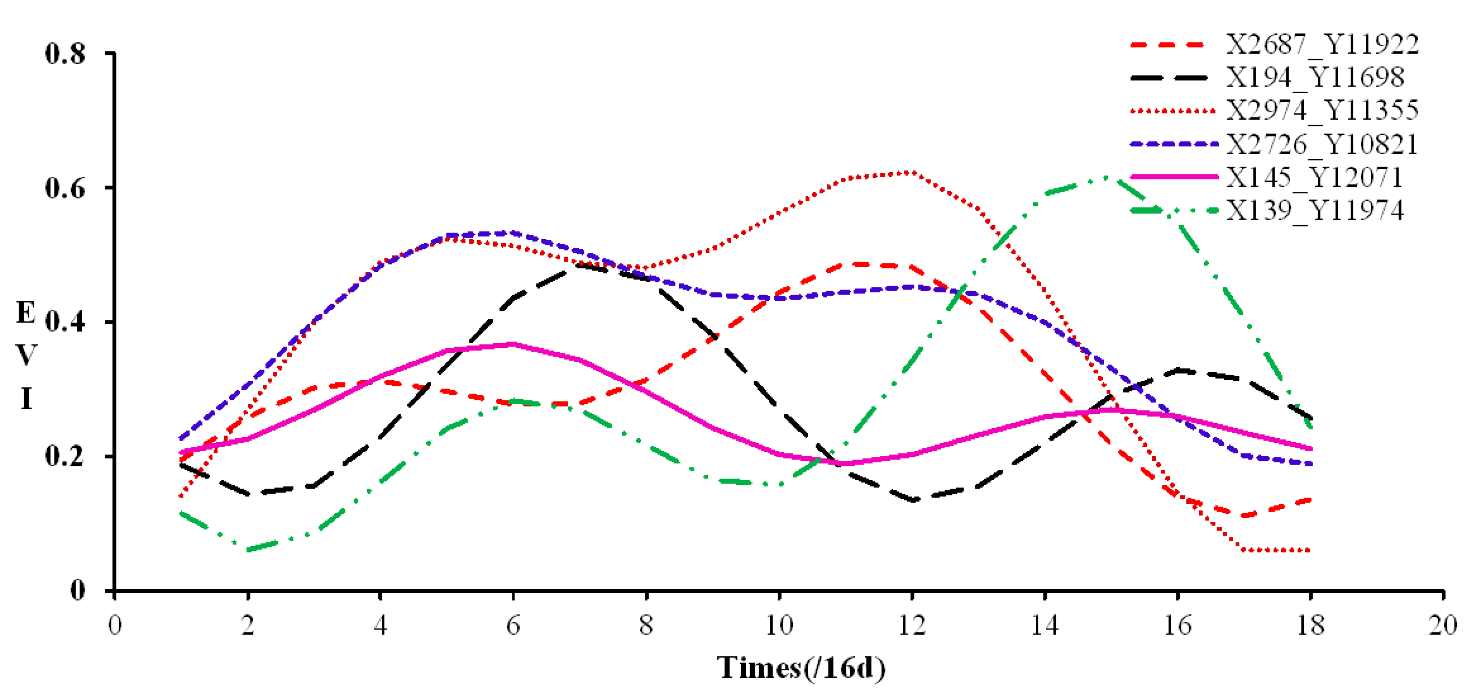
2.2.1. Harmonic Analysis of Time Series

There are many methods for time series data reconstruction [42,43,44]. Among them, the Harmonic ANalysis of Time Series (HANTS) and TIMESAT [45], which have software package support, are commonly used. The HANTS has advantages for dealing with the time series of irregularly spaced observations and for identifying and removing cloud-contaminated observations [46]. The TIMESAT program uses an adaptive Savitzky-Golay filtering method and developed methods that are based on upper envelope weighted fits to asymmetric Gaussian and double logistic model functions [45,47]. The TIMESAT has a high processing efficiency, but it has limitations on the selection of algorithms. Compared with the TIMESAT, the disadvantage of the HANTS is that there are no objective rules for determining the control parameters; thus, this determination is made on the basis of experience and after running several combinations of control parameters [46]. However, because the cropland distribution has obvious irregular features that are affected by human activities, the HANTS was selected as the primary method for time series construction in this study.
The core of the harmonic analysis is the Fourier transform and least squares fitting. Using a discrete Fourier transform, the time series of an element is transformed from the time domain to the frequency domain. A harmonic (sinusoidal) wave exists in the time domain that corresponds to each frequency component. Time series data can be decomposed into different harmonic curves of frequency using HANTS. Typical curves that reflect the time series are selected and superposed consequently. Time series data can then be reconstructed. The theory of HANTS is as follows:
f ( x ) = A 0 + i = 1 A i sin ( ω i x + φ i )
where f(x) is the continuous time series curve that satisfies the hypothesis of the convergence theorem (Dirichlet) and 2t cycle, A0 is a harmonic reminder, i is the order of harmonic, Ai is the amplitude of the harmonic order i, ωi is the frequency of the harmonic order i, and φi is the phase of the harmonic order i.
The Fourier expansion is as follows:
f ( x ) = a 0 2 + i = 1 ( a i c o s ω i x + b i s i n ω i x ) A 0 = a 0 2 = 1 t t t f ( x ) d x ,   a i = 1 t t t f ( x ) c o s ω i x d x ,   ( i = 1 , 2 , ) ,   b i = 1 t t t s i n ω i x d x , ( i = 1 , 2 )   A i = a i 2 + b i 2 , ω i = π i t , φ i = a r c t a n a i b i
where ai, bi are the Fourier coefficients of harmonic order i. A Fourier coefficient is fit using the least squares method as follows:
M T × M × J = M T × Y
where J is the coefficient matrix, M is the Fourier matrix, and MT is the transposed matrix of the Fourier matrix. The coefficient matrix can be computed using the Fourier fitting process, as has been elucidated in detail in previous research [48,49,50].

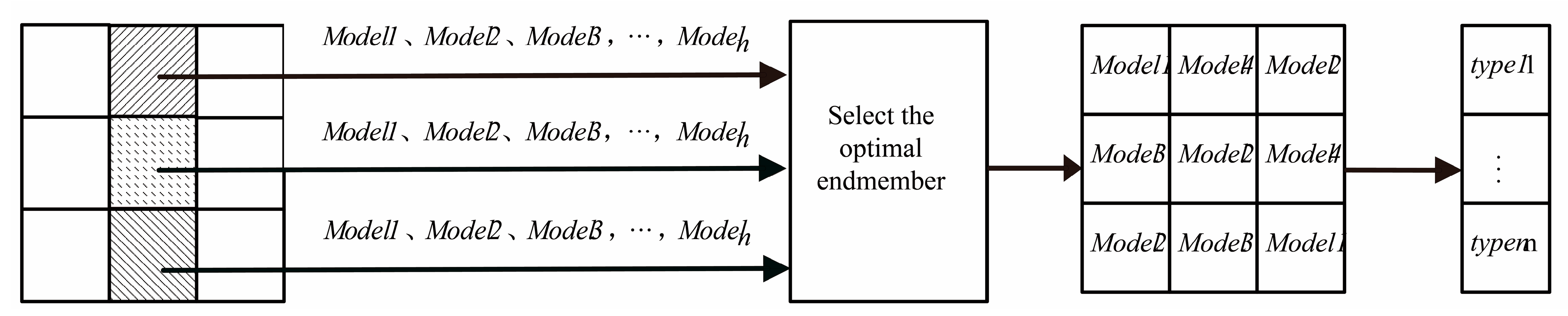
2.2.2. Multiple Endmembers Spectral Mixture Analysis

The mixed pixels of a land cover image indicate that a pixel is composed of several different pure land cover types. The spectrum value of a mixed pixel is the mix value of the pure land cover types in this pixel. Each spectrum value of the pure land cover type is called an endmember. The Linear Spectral Mixture Model (LSMM), which is widely used when quantitatively extracting land cover information [51], is used to extract the endmember in a mixed pixel. Based on the time series data extracted from the EVI using HANTS, the endmembers were selected by the linear mixture model, which is as follows:
P j = i = 1 N c i e i , j + r j
i = 1 N c i = 1 ,   0 c i 1
RMSE = j = 1 M r j 2 M
where N is the number of endmembers, M is the number of bands, Pj is the reflectance of bands j, and ci is the fraction of the endmember in the pixel. ei,j is the reflectance of endmember i in band j, and rj is the residual. The RMSE (root mean square error) is used to evaluate the accuracy of the model’s fit.
A Multiple Endmember Spectral Mixture Analysis (MESMA) is an advanced model that is based on the LSMM [52], and allows endmembers to vary on a per-pixel basis. The optimal linear endmember combination can be selected by comparing multiple endmember models in one mixed pixel based on the MESMA. Terrain shade is considered an endmember in the MESMA and can increase the accuracy of the model [53]. Vegetation and shade constitute a two-endmember model called the vegetation-shade model, and vegetation, cultivated land and shade constitute a three-endmember model called the vegetation-cultivated land-shade model. The endmember composition principle of MESMA is shown in Figure 2. Model1, Model2, ..., and Modeln in Figure 2 represent different endmember models. The endmember model may be a two-endmember, three-endmember, four-endmember, …, n-endmember model, where n is a variable.
Figure 2. Multiple Endmember Spectral Mixture Analysis principle.
Remotesensing 06 11708 g002
All of the models are run for each pixel. For example, after running m two-endmember models, if the RMSE in a pixel located in (100, 100) is RMSE1 < RMSE4 < RMSEm-2 < ... < RMSEm, with the smallest value being the RMSE1, the type of the pixel (100,100) can be interpreted as vegetation because the two-endmember model is vegetation-shade. All of the pixels can be interpreted by repeating this process. The cultivated land information reported in the paper was derived using the two-endmember model.
2.2.3 Endmember Selection
Endmember selection is the most important step in the decomposition of mixed pixels. There are traditionally two methods for selecting endmembers: the image endmember method and the reference endmember method. The former method allows the selection of homogeneous pixels directly from actual images, which is more likely to be used with the actual geographic features in the field. The latter method poses difficulty for ensuring the synchronization of the measured data and the actual image data. Moreover, it is difficult to guarantee the appropriate correction of the atmosphere correction. The image endmember method is more commonly used in research activities than the reference endmember method [54]. Taking the year 2000 as an example and using the image endmember method, the selection process is described as follows: (1) Perform a Minimum Noise Fraction (MNF) transformation based on the composite image. In this case, most of the information is concentrated in the first five MNF bands. (2) Label the Pure Pixel Index (PPI) of every pixel in the processed image. (3) Build an image endmember library based on the above labeled pixels and position the endmembers on Google Earth promptly. As a result, the image endmember library will be built.

2.2.4. Accuracy Assessment Method

The fit of a model is generally assessed using the residual and RMSE over all of the image bands. The interpreted cultivated land data are quantitatively evaluated, and the coefficient of spatial consistency is evaluated in space. The coefficient of spatial consistency can be computed by comparing the reference data and interpreted data pixel by pixel. The formulas are as follows:
K t o t a l = 1 | A i n t e r p r e t e d A r e f e r e n c e | A r e f e r e n c e × 100 %
where Areference is the reference cultivated land area, Ainterpreted is the interpreted cultivated land area, and Ktotal is the overall accuracy.
K = M M + N
where K is the coefficient of the space consistency, M is the number of pixels with consistent spatial attributes, and N is the number of pixels with inconsistent spatial attributes [55].

3. Results

3.1. Time Series Data Reconstruction

The vegetation-related information was commonly found in low frequency harmonics. Meanwhile, the noise of the handling errors generated in the process generally existed in the higher frequency harmonics. To reduce these noise effects, we set the inhibition of the direction to “low” in this study using HANTS to exclude the high frequency harmonics and to reconstruct the smooth low frequency harmonics. With repeated testing and analysis, the MOD13Q1/EVI time series data in the NSTNEA were reconstructed for 2000 and 2010. The frequency was set to two, and the error tolerance and degree of over determinedness were set to 1000 and eight, respectively.
Figure 3 shows the curves before and after the time series data reconstruction. The blue curve represents the original curve, which has a serrate wave. The red curve represents the constructed curve, which reflects the actual changes more realistically. Figure 4 shows the different cropland EVI curves in the different locations (X, Y) of the transect after HANTS processing. These fluctuation curves may reflect the double cropping and various phenology characteristics. These features are helpful for the endmember selection and cropland information extraction.
Figure 3. EVI time-series curves before and after a harmonic analysis.
Remotesensing 06 11708 g003
Figure 4. Cultivated land characteristic library.
Remotesensing 06 11708 g004

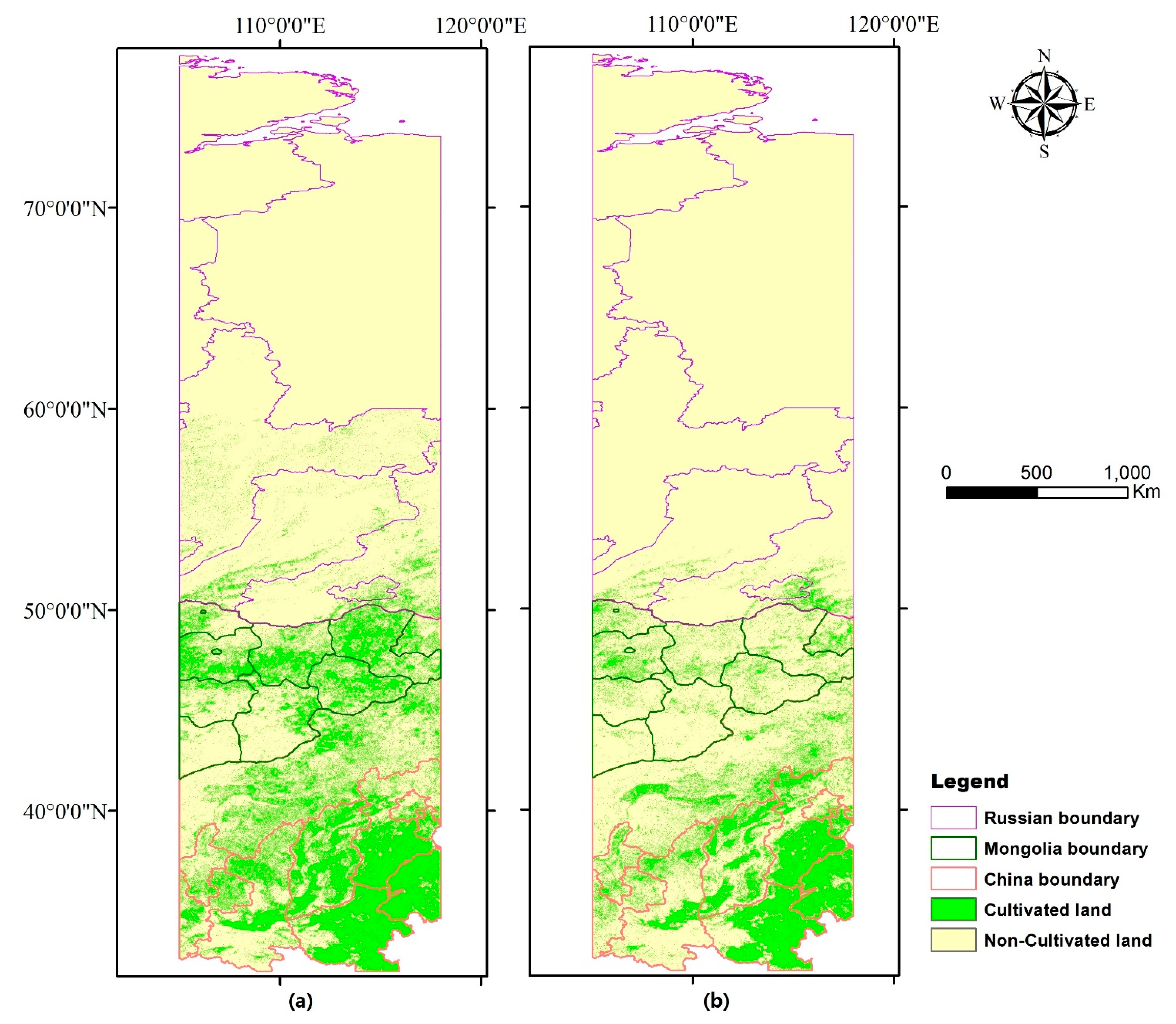
3.2. Cultivated Land Information Extraction

The basic principle of sample point selection is to ensure that every province in each country has a similar number of points (endmembers) of different types. Combined with PPI and the MODIS images of 2000 and 2010, the authors selected cultivated and non-cultivated points from Google Earth. All of the selected endmembers were integrated into the image spectrum feature library, which includes 643 cultivated land points, 284 non-vegetation points and 827 vegetation points for the year 2000 and 449 cultivated land points, 661 non-vegetation points and 729 vegetation points for the year 2010. A total of 1754 curves for 2000 and 1839 for 2010 were selected (Figure 5). Using the image spectrum feature library, two-endmember models were built that combined the features of endmember and shade. All of the models were classified into three categories: cultivated land-shade, vegetation-shade, and other-shade (other-shade represents the land cover other than cultivated land and vegetation). Shade is taken as an endmember only at the sub-pixel level and not used directly for cultivated land extraction. It is part of the accuracy assessment because the results and the reference data must be compared at the pixel level.
Figure 5. Sample distribution in the NSTNEA in 2000 and 2010.
Remotesensing 06 11708 g005
The two-endmember models are run pixel by pixel. The model with the least RMSE is then selected. The cultivated land is extracted based on the model’s calculation for 2000 and 2010. However, it is difficult to distinguish some of the cultivated land from the vegetation in Russia using the cultivated land distribution results because the highest EVI values for both the cultivated land and the forests are all from 0.25 to 0.3 in the alpine range region. In this case, the DEM and Google Earth images were selected as auxiliary data to extract the cultivated land in the Russia area. We hypothesized that the cultivated land in Russia exists where the DEM ranges from 500 m to 1000 m. Russia’s cultivated land was extracted and is primarily distributed in the Republic of Buryatia and outside Baikal Lake. The final results of the cultivated land distribution for the years 2000 and 2010 are shown in Figure 6a,b, respectively.
Figure 6. The distribution of cultivated land in the NSTNEA in 2000 and 2010.
Remotesensing 06 11708 g006

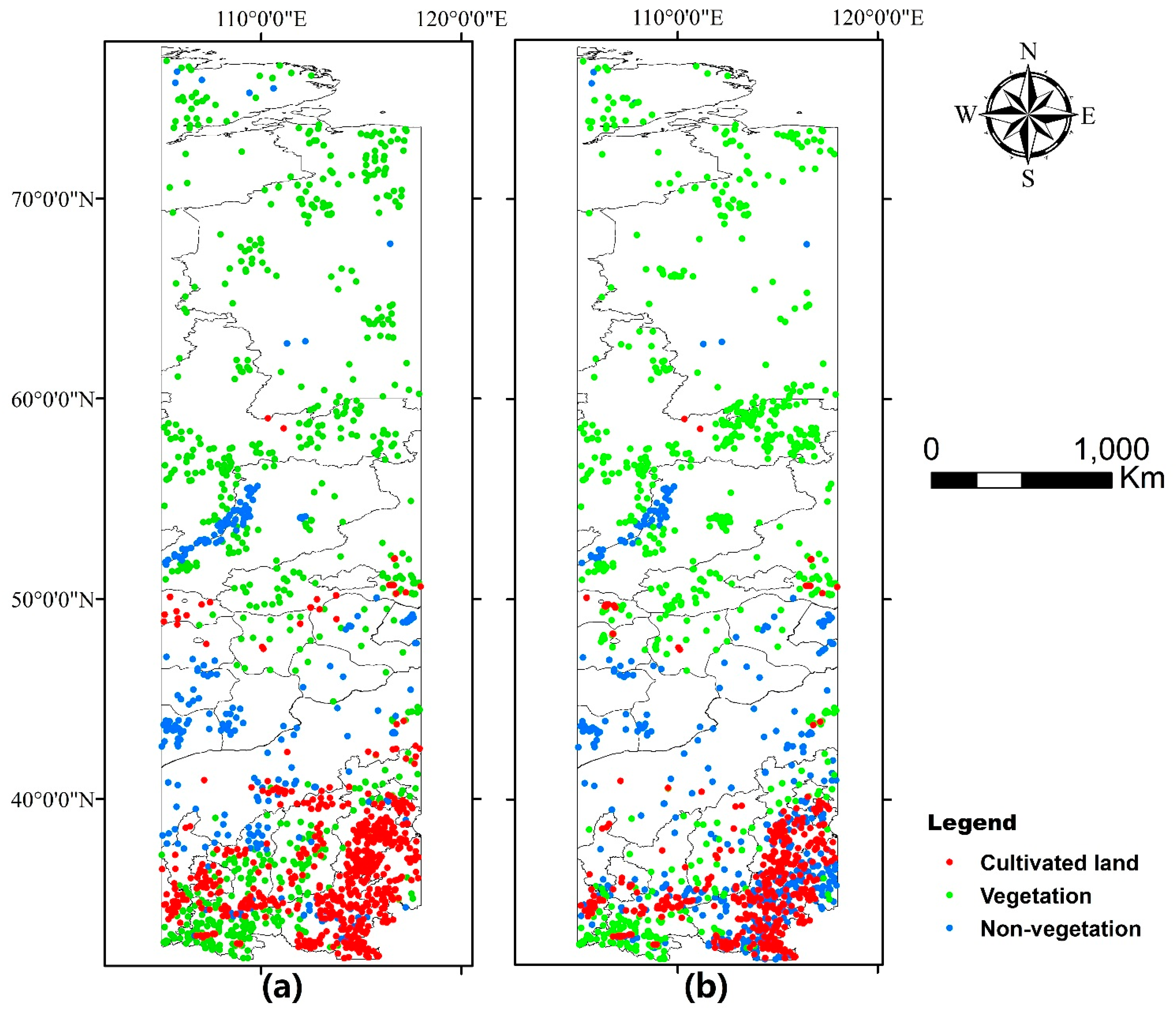
3.3. Accuracy Assessment

3.3.1. Model Accuracy

(1) Model Accuracy Assessment in 2000

The distribution range of the absolute values of residuals (Table 3) and the RMSE (Table 4) was computed for each band. More than 99.5% of the pixels had absolute residuals less than 0.1, as shown in Table 3. More than 98% of the pixels with RMSEs were less than 0.05, as shown in Table 4. These results suggest that the decomposition error of the model is very small.
Table 3. Distribution range of residuals in 2000.
Range (%)T1T2T3T4T5T6T7T8T9
0–0.199.54999.52899.477699.457299.482199.486599.507699.568499.5913
0.1–0.20.39790.41180.4490.45830.43670.44170.44320.38810.3653
0.2–0.30.04050.04220.04940.05890.05520.05440.04020.03580.0364
0.3–0.40.00570.01020.01190.01290.01470.01220.0070.00650.0048
0.4–0.50.00150.00360.00620.00630.00620.00330.00080.00080.0019
>0.50.00310.00440.0060.00620.00390.0009000.0002
Range (%)T10T11T12T13T14T15T16T17T18
0–0.199.59199.699.675599.650299.546199.393499.362299.475199.6236
0.1–0.20.35870.35970.29570.31850.40220.51380.52310.4430.3176
0.2–0.30.04340.03650.02440.0260.04020.07580.0930.06210.042
0.3–0.40.0050.00410.00370.00370.00880.01280.01760.01280.0102
0.4–0.50.00180.00020.00030.00080.00220.0030.00290.00370.0024
>0.500000.00040.00080.00110.00380.0045
Table 4. Distribution range of RMSEs in 2000.
Range0–0.050.05–0.10.1–0.150.15–0.20.2–0.250.25–0.30.3–0.35>0.35
Percent %98.11761.50120.2750.06930.01910.00850.00370.0051

(2) Model Accuracy Assessment in 2010

Table 5 and Table 6 show the statistical results for the residuals and RMSEs in 2010. The decomposition error of the model is similar to that in 2000. More than 99% of the pixels with absolute residuals were less than 0.1, and more than 98% of the pixels with RMSEs were less than 0.05.
Table 5. Distribution range of the 2010 residuals.
Range (%)T1T2T3T4T5T6T7T8
0–0.199.4699.560599.539999.579999.492399.383899.425299.5847
0.1–0.20.39740.38810.42350.3790.44660.5690.52830.386
0.2–0.30.02830.03890.02850.03180.05150.03960.04350.0261
0.3–0.40.00970.00780.0060.00740.0080.00580.00250.0024
0.4–0.50.00470.00260.00120.00110.0010.001100.0001
>0.50.00720.00420.00120.00110.0010.001100.0001
Range (%)T9T10T11T12T13T14T15T16
0–0.199.66199.66199.647299.679899.596899.437399.427599.4788
0.1–0.20.30920.30920.33390.29870.36560.51220.50990.4606
0.2–0.30.02620.02620.01430.01740.03430.04360.04930.0433
0.3–0.40.00250.00250.00350.00340.00260.0060.00970.0109
0.4–0.50.00020.00020.0005000.00060.00230.0042
>0.50.00020.00020.0005000.00060.00250.0057
Table 6. Distribution range of the 2010 RMSEs.
Range0–0.050.05–0.10.1–0.150.15–0.20.2–0.250.25–0.30.3–0.35>0.35
Percent %98.11761.50120.2750.06930.01910.00850.00180

3.3.2 Cultivated Land Accuracy

The overall accuracy and spatial consistency coefficient were used to assess the accuracy of the results. The results are shown in Table 7. In the NSTNEA, using the GLC2000 and GlobCover2009 as references, the overall accuracy and spatial consistency coefficients were 81.63% and 0.78 in 2000 and 72.81% and 0.75 in 2010, respectively. To further verify the method, the more precise NLCD-2000 was used in the Chinese region of the transect. The overall accuracy and spatial consistency coefficients were 94.76% and 0.79, respectively.
Table 7. Accuracy assessment.
GLC2000GlobCover2009NLCD-2000
Overall Accuracy72.81%83.16%94.76%
Spatial Consistency Coefficient0.780.750.79
The small residual and the RMSE show that the decomposition result of the model is reliable [56]. As for the cultivated land precision, the overall accuracy demonstrates high consistency with the land cover data products of the global scale and has a high accuracy in the Chinese part of the transect. It is worth mentioning that the original land cover products have the limitations noted above and inherent disagreements exist in regard to the cultivated land cover type [36]. However, the high spatial consistency coefficient suggests that the results are feasible for further spatial distribution and gradient analyses for 2000 and 2010 in this large transect scale.

4. Discussion

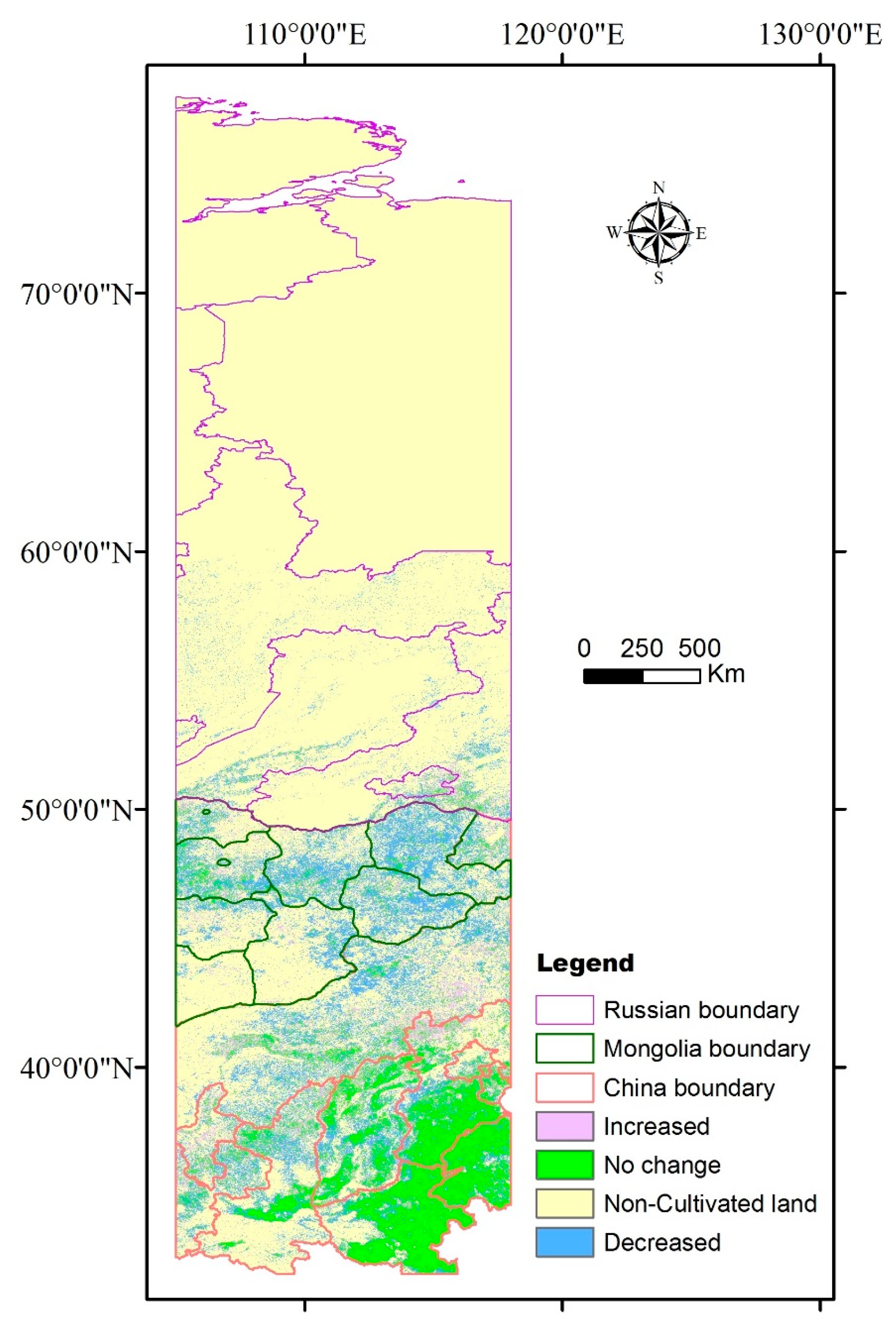
4.1. Spatial Distribution Analysis

In 2000, the spatial distribution of the cultivated land shows that the pattern is centralized in the southeast and decentralized in the northwest. The distribution range mainly includes the northeastern Henan province, western Shandong province, southern Hebei province, central Shaanxi province and Shanxi province. There are also sporadic distributions of cultivated land in the northern Hebei province, southern Shaanxi province, eastern Gansu province, northwestern Henan province, Inner Mongolia and the Ningxia autonomous region. In Mongolia, the cultivated land is mainly distributed in the northeast area. Most of the cultivated land is distributed in the Ulaanbaatar, Dornod, Sukhbaatar, Khentii and Central provinces. In Russia, the cultivated land is primarily distributed in the Republic of Buryatia and outside Baikal Lake. There is little cultivated land in the northern Irkutsk region. In general, the pattern of the transect in 2000 is as follows: the cultivated land is distributed primarily in the south, while almost no cultivated land resources are in the north. Most of the cultivated land is distributed in China, followed by Mongolia and then Russia. Although the general distribution pattern of the cultivated land in 2010 is consistent with that in 2000, the total area of the cultivated land and locations of the regional distributions changed dramatically.
According to the statistics, the cultivated land accounted for 6.57 × 10⁷ ha in China, 2.07 × 10⁷ ha in Mongolia, and 0.56 × 10⁷ ha in Russia in 2000. In 2010, the cultivated land accounted for 5.10 × 10⁷ ha in China, 0.73 × 10⁷ ha in Mongolia, and 0.23 × 10⁷ ha in Russia. The spatial distribution of the change in the cultivated land is illustrated in Figure 7. The magenta represents the regions with an increase in cultivated land, and the blue represents areas with a decrease in cultivated land between 2000 and 2010. The figure shows that the increasing cultivated land area is less than the decreasing cultivated land area. The cultivated land in the total transect decreased 34.16%. Regionally, the cultivated land decreased by 22.37%, 58.93%, and 64.73% in China, Russia, and Mongolia, respectively.
Figure 7 shows the loss of cropland that is apparent in locations higher than 53°N in the Russia area and near 48°N in the eastern area of Mongolia. The reasons for the loss of cropland are attributed as follow: In the Russian region, we used the elevation as a condition parameter for cropland detection, which may have resulted in an underestimation of the cropland area. Additionally, in the Mongolian area, the amount of abandoned land increased significantly after the changes to Mongolia’s economic system in 1991 [57]. Thus, the cropland that was abandoned in the years immediately following 2000 is not easily distinguished from the grassland, although this distinction is clear in 2010. This phenomenon may have caused the amount of cropland to be overestimated in 2000 and explain the dramatic decrease between 2000 and 2010.
Figure 7. Changes in the cultivated land in the NSTNEA between 2000 and 2010.
Remotesensing 06 11708 g007

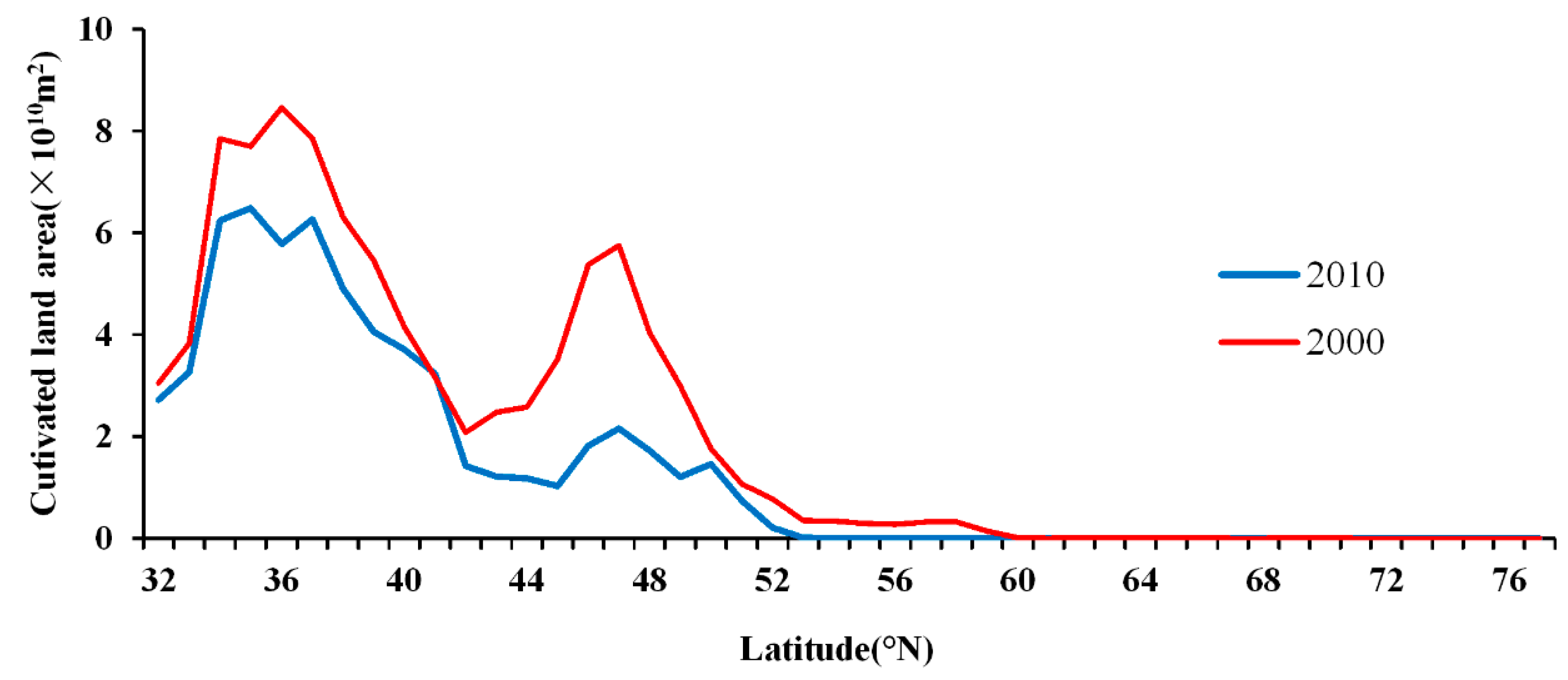
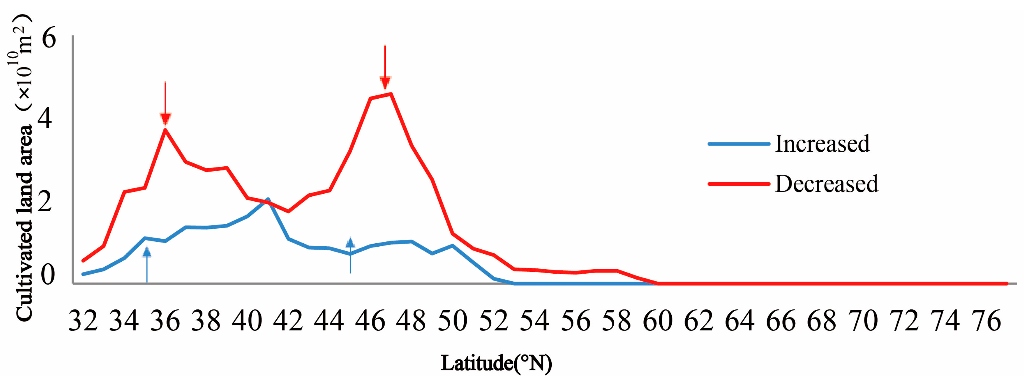
4.2. Gradient Analysis

To identify the gradient distribution and the change characteristics of the cultivated land in the transect from the south to the north, the transect was divided into 46 latitudinal gradient zones with 1° intervals. The area of the cultivated in each gradient zone was counted. Figure 8 shows the latitudinal graded distribution of the cultivated land in 2000 (the red colored curve). The curve shows a sinusoidal wave shape, and the entire change shows a “High-Low-High-Low” mode. The main transition region is between 32°N and 52°N. The cultivated land distribution gradually increases from 32°N and reaches its first peak at 36°N. The main bread basket is located in northern China, including the eastern Loess Plateau and the western North China Plain. From 37°N to 42°N, the area of cultivated land is drastically reduced. The primary region is located in a farming-pastoral ecotone in northern China that includes the northern Ningxia province, northern Shanxi province, northern Shaanxi province, Hebei province, and Inner Mongolia Autonomous Region. The amount of cultivated land in the region near 42°N is small because of the large steppe and Gobi that are distributed in the trans-boundary region of China and Mongolia. The amount of cultivated land increases from 42°N to 47°N and reaches its second peak in the transect with the Dornod province, Khentii province, Central province and Ulaanbaatar having a relatively large cultivated land distribution in Mongolia. Among them, the Central province and Ulaanbaatar have the largest cultivated land distribution in Mongolia near 47°N. From 47°N to 58°N, there is a sharp decline in the cultivated land area, especially above 54°N, where little cultivated land exists. The junction of Mongolia and Russia is adjacent to 50°N. The cultivated land in this area is very small and is scattered throughout the Russian region, except for the Republic of Buryatia and outside Baikal Lake from 52°N to 58°N.
Figure 8. The latitudinal graded distribution of the cultivated land in 2000 and 2010.
Remotesensing 06 11708 g008
The latitudinal graded distribution of the cultivated land in 2010 is illustrated in Figure 8 (the blue colored curve). This curve also shows a sinusoidal wave shape, and the entire change shows a “High-Low-Middle” mode. The change mainly occurs between 32°N and 52°N. The distribution pattern in China is similar to that in 2010, but it is clearly different in Mongolia from 42°N to 50°N. The cultivated land area curve peak in the Central province and Ulaanbaatar clearly decreases, causing a dramatic fluctuation in its neighboring region. There is little cultivated land north of 50°N, especially above 52°N in Russia.
The gradient change in the cultivated land between 2000 and 2010 shown in Figure 9 demonstrates the obvious fluctuations in the amount of cultivated land, with both increasing and decreasing features. For our purposes, increasing means that the non-cropland was converted into cropland, and decreasing means that the cropland became non-cropland. The change curve shows that the main trend is decreasing with two sharp peaks. One peak occurs at 36°N, which is the location of the “Grain for Green” project implementation area in the Loess Plateau of China. The related regions near this decreasing peak include Gansu, Shaanxi, Shanxi, and Shandong provinces. In this location, potatoes, beans and wheat are widely cultivated. The other peak occurs at 47°N, where the capital of Mongolia is located. The related regions near this second peak include the Ulaanbaatar, Central, Sukhbaatar, and Khentii provinces of Mongolia, in which potatoes and wheat are widely cultivated. The decreasing area covers nearly all of the Mongolia area in the transect. The total decreasing cultivated land area is approximately 0.3 × 10⁷ ha between the two decreasing peaks. There is also an increased peak in the cultivated land in the transect, but the peak value is a bit lower. A flat peak exists near 40°N, where limited cultivated land in the trans-boundary area between China and Mongolia is distributed. In this region, the area of the corn and beans that is cultivated increases in the Chinese region, while the area of the cultivated potatoes and wheat decreased in the Mongolia region. Overall, the area of cultivated land decreased dramatically between 2000 and 2010.
Figure 9. The latitudinal gradient distribution of cultivated land in 2000 and 2010.
Remotesensing 06 11708 g009

4.3. Analysis of the Driving Forces Changing the Cultivated Land

Generally, the driving forces of the changes in the cultivated land in the transect can be attributed to both natural and human factors. Local physical geographic conditions and climate change directly influence the distribution of the cultivated land. The temperature and precipitation have obvious gradient features from the south to the north. These two factors are important natural influences on the growth of crops and the reasons why the cropland is mainly distributed in the southern region, decreases with increasing latitude, and remains small in the northern region of the transect [57]. Although the natural driving forces can strongly affect the spatial distribution of the cultivated land, they were not the cause of the dramatic changes in the different countries during the 10-year study period, as the trans-boundary area of the three countries has a continuous and integrated ecological environment. Therefore, human activities as the driving forces of cultivated land change are analyzed and discussed in detail in this section.
In China, the implementation of the Reform and Opening policy and the socialist market economic system impacted the distribution of cultivated land as a result of a series of regional development strategies in northern China, such as the Western Development and Central Rise policy. Additionally, a series of ecological construction engineering projects have been initiated since the 1990s. The primary reasons for China’s cultivated land changes from 2000 to 2010 are discussed below, considering the current social background. First, with the acceleration of urbanization, large areas of cultivated lands have become occupied. Approximately 55.44% of the reduction of cultivated land in China from 2000 to 2010 was due to its use for construction [58]. Second, with the development of the economy, a large rural population moved to the cities, abandoning their cultivated lands. This migration inevitably led to the reduction of the total area of cultivated land. Third, many large-scale and long-term ecological construction projects were performed. For example, the Conversion from Cropland to Forest and Grassland Program (also called “Grain for Green, GFG”), which was initiated by the government in 1999, is a cropland retirement program with the integrated objectives of ecological preservation and local development. In 2002, 1897 counties in 25 provinces implemented a GFG policy. Most of these counties are either fully or partially included in the transect. To ensure crop security, the Chinese government protected the integral farmland with national policies; thus, although the area of cultivated land decreased on the whole, a small increasing trend still exists in the transect.
In Mongolia, the accelerated urbanization process and the declining rural population since the 1980s has increased the abandonment of cultivated land. After the reform of Mongolia’s social and economic systems in 1991, the agricultural policy changed from centralization to a free market economy. This weakened the centralized market and reduced support for agricultural investments both directly and indirectly. Because of a lack of effective marketing management and a functioning market economy, Mongolia’s agricultural production experienced an economic transition resulting from the following [59]: (1) instability of the market, (2) policy change, and (3) unclear land-use policies. These uncertainties affected agricultural production and led to the abandonment of farmland. The lack of machinery and of an irrigation management infrastructure also caused a decline in the crop yields. For example, in 2004, 138.5 thousand tons of cereals, 80.2 thousand tons of potatoes, 49.0 thousand tons of vegetables, and 9.6 thousand tons of fodder crops were produced. These levels of cereal and potato production are equivalent to an average of 17.5% and 75.3% of the level prior to 1990, respectively [60].
In Russia, national policies and the economic system were the primary factors for the reduction in cultivated land. The Russian Federation enacted a series of laws and established a number of nature reserves in the region to protect its resources as a precondition for economic development. After the dissolution of the Soviet Union in 1991, however, the Russian government launched rural land privatization as a core agricultural reform. The country ceased providing direct financial subsidies for agricultural production after enacting the policy with the result that some farmers chose to reduce their production, thereby causing a large area of cultivated lands to become idle. The data show that 120.9 million hectares of land were cultivated in 1999 and 76.36 million hectares of land were cultivated in 2007, indicating that the privatization of the rural land resulted in a decline in the area under cultivation [61,62,63]. The continuing decrease in the population is an important reason for the loss of farmland in Russia.

5. Conclusions

This study aimed to obtain information about the cultivated land using a mixed pixel model and yearly time series data in the transect. The method, which combines HANTS, LSMM, MNF, and PPI, can automatically derive cultivated land with pixel-level accuracy and may provide cost-effective means of mapping cultivated land with a large spatial coverage. The extracted cultivated land was divided into gradient zones in this transect in 2000 and 2010. Additionally, we qualitatively analyzed the arable gradient distribution and described the changes between 2000 and 2010. By analyzing the driving forces of the cultivated land change, we concluded that policy transformations were the predominant reasons for a decrease in the amount of cultivated land.
However, some points remain for study in the near future. First, the data processing method used in this study could be improved. As previously mentioned, TIMESAT is another good method for time series data construction and our next step is to compare it with the method we used here. Second, the distribution of the continuously cultivated land in the transect by year is also a future area of study that may yield more details about the changing trends in this trans-boundary area.

Acknowledgments

This work was supported by CAS Key Deployment Project (KZZD-EW-08-02-03), Science & Technology Basic Research Program of China (2007FY110300, 2011FY110400, and 2013FY114600), Specific Informational Infrastructure Program of CAS (XXH12504-1-01) and Talent Special Projects of Russia, Ukraine, White Russia, CAS, National Science and Technology Infrastructure of China (2005DKA32300). The authors would like to thank the editor and all the reviewers for their helpful suggestions and comments on this paper.

Author Contributions

Juanle Wang drafted the manuscript and was responsible for the research design. Yujie Zhou was responsible for the data processing and results analysis. Lijun Zhu supported the data preparation. Mengxu Gao and Yifan Li provided some useful suggestions on data processing and results analysis. All of the authors contributed to editing and reviewing the manuscript.

Conflicts of Interest

The authors declare no conflict of interest.

References

  1. Wang, J.-L.; Song, J.; Zhu, L.-J. Construcion of resource and environment science expedition data resource integration system in Northeast Asia. J. Geoinf. Sci. 2012, 14, 74–80. [Google Scholar]
  2. Wang, J.-L.; Zhu, L.-J.; Sun, C.L. Study and implementation on multi dimension data management model in integrated resources and environment scientific expedition—Case in integrated scientific expedition in North China and its neighboring area. J. Nat. Res. 2011, 26, 1129–1138. [Google Scholar]
  3. Wang, J.-L.; Zhu, L.-J.; Yang, Y.; Zhang, L. Design, development and application of Northeast Asia resources and environment scientific expedition data platform. J. Resour. Ecol. 2011, 2, 266–271. [Google Scholar]
  4. Deng, J.-S.; Wang, K.; Shen, Z.-Q.; Xu, H.-W. Decision tree algorithm of automatically extracting farmland information from SPOT-5 images based on characteristic bands. Trans. Chin. Soc. Agric. Eng. 2004, 20, 145–148. [Google Scholar]
  5. Stern, A.J.; Doraiswamy, P.C.; Akhmedov, B. Techniques for developing land-use classification using moderate resolution imaging spectroradiometer imagery. J. Appl. Remote Sens. 2009, 3. [Google Scholar] [CrossRef]
  6. Li, X.-C.; Xu, X.-G.; Wang, J.-H.; Wu, H.-F.; Jing, X.-L.; Li, C.-J.; Bao, Y.-S. Crop classification recognition based on time-series images from HJ satellite. Trans. Chin. Soc. Agric. Eng. 2013, 29, 169–176. (In Chinese) [Google Scholar]
  7. Hou, G.-L.; Zhang, H.-Y.; Wang, Y.-Q.; Zhang, Z.-X. Application of harmonic analysis of time series to extracting the cropland resource in Northeast China. J. Nat. Res. 2010, 9, 1607–1617. [Google Scholar]
  8. Wang, H.-S. Arable Land Information Extraction Using MODIS Multi-Temporal Data. Ph.D. Thesis, Zhejiang University, China, 2008. [Google Scholar]
  9. Bai, M.; Liu, H; Huang, W.; Qiao, Y.; Mu, X. Automatic farmland extraction from multi-temporal Landsat TM data based on artificial neural network. In Proceedings of 2009 Inernational Conference on Geoinformatics, Fairfax, VA, USA, 12–14 August 2009; pp. 1–4.
  10. Bruzzone, L.; Cossu, R. A multiple-cascade-classifier system for a robust and partially unsupervised updating of land-cover maps. IEEE Trans. Geosci. Remote Sens. 2002, 40, 1984–1996. [Google Scholar] [CrossRef]
  11. Liu, X.-S.; Sun, R.; Wu, F.; Hu, B.; Wang, W. Land-cover classification for Henan Province with time-series MODIS EVI data. Trans. Chin. Soc. Agric. Eng. 2010, 26, 213–219. (In Chinese) [Google Scholar]
  12. Tang, Y.; Yang, W.-N.; Li, J.; Dai, X.-A. A study of information extraction based on QuickBird data—Taking the extraction of cultivated land for an example. In Proceedings of 2010 International Conference on Multimedia Technology (ICMT), Ningbo, China, 29–31 October 2010; pp. 1–4.
  13. Zhu, L.; Wu, B.-F.; Zhou, Y.-M.; Zhang, L.; Zhang, N. Object-oriented land cover information extraction in emigration area of Zigui county using high resolution imagery. In Proceedings of 2009 Joint Urban Remote Sensing Event, Shanghai, China, 20–22 May 2009; pp. 1–6.
  14. Peña-Barragán, J.M.; Ngugi, M.K.; Plant, R.E.; Six, J. Object-based crop identification using multiple vegetation indices, textural features and crop phenology. Remote Sens. Environ. 2011, 115, 1301–1316. [Google Scholar] [CrossRef]
  15. Vintrou, E.; Desbrosse, A.; Bégué, A.; Traoré, S.; Baron, C.; Lo Seen, D. Crop area mapping in West Africa using landscape stratification of MODIS time series and comparison with existing global land products. Int. J. Appl. Earth Obs. Geoinf. 2012, 14, 83–93. [Google Scholar] [CrossRef]
  16. Dewan, A.M.; Yamaguchi, Y. Using remote sensing and GIS to detect and monitor land use and land cover change in Dhaka Metropolitan of Bangladesh during 1960–2005. Environ. Monit. Assess. 2009, 150, 237–249. [Google Scholar] [CrossRef] [PubMed]
  17. Yan, F.; Liu, D.-Z.; Wang, Y.-M. Visual interpretation’s applying on land-use types investigation based on QuickBird image—A case study in Xinqiao town of Chuanshan District in Suining City. Environ. Prot. Xinjiang 2008, 30, 6–10. (In Chinese) [Google Scholar]
  18. Liu, K.-B. Precision analysis of rice-planting area in Heilongjiang Province by visual image interpreting applying satellite SPOT4 and SPOT5 images. Heilongjiang Agric. Sci. 2011, 5, 118–120. (In Chinese) [Google Scholar]
  19. Dou, Y.-X.; Zhao, G.-X.; Tian, W.-X.; Zhang, Y.-H. Study on automatic abstraction techniques of cultivated land information on county level by satellite remote sensing. China Popul. Resour. Environ. 2000, 10, 116–118. [Google Scholar]
  20. Zhao, G.-X.; Dou, Y.-X.; Tian, W.-X.; Zhang, Y.-H. Study on automatic abstraction methods of cultivated land information from satellite remote sensing images. Sci. Geogr. Sin. 2001, 21, 224–229. [Google Scholar]
  21. Miller, R.L.; McKee, B.A. Using MODIS Terra 250 m imagery to map concentrations of total suspended matter in coastal waters. Remote Sens. Environ. 2004, 93, 259–266. [Google Scholar] [CrossRef]
  22. Wang, Q. Advance research on terrestrial transects. Adv. Earth Sci. 1997, 12, 43–50. [Google Scholar]
  23. Hong, J.; Wang, J.-L. Transect Expedition and Thematic Expedition Data Integration Report; Institute of Geographic Sciences and Natural Resources Research, Chinese Academy of Sciences: Beijing, China, 2012. [Google Scholar]
  24. Diao, L.-M.; Fan, Y.-L. Structural crisis of the Russian population. Siberian Stud. 2007, 34, 5. [Google Scholar]
  25. Li, S.; Liu, W.-D. Spatial distribution of population in Russia and its evolution. Econ. Geogr. 2014, 34, 8. (In Chinese) [Google Scholar]
  26. Narantungalag, B. Research on Population Development in Mongolia. Ph.D. Thesis, Jilin University, Changchun, China, 2012. [Google Scholar]
  27. Ren, X.-J. Empirical analysis of the Sino-Mongolian economic and trade cooperation in the Mongolian side factors. Econ. Forum 2009, 455, 129–132. (In Chinese) [Google Scholar]
  28. Zuo, L.-J.; Zhang, Z.-X.; Dong, T.-T.; Wang, X. Application of MODIS/NDVI and MODIS EVI to extracting the information of cultivated land and comparison analysis. Trans. Chin. Soc. Agric. Eng. 2008, 24, 167–172. (In Chinese) [Google Scholar]
  29. National Aeronautics and Space Administration. http://modis.gsfc.nasa.gov/ (accessed on 30 January 2013).
  30. Land Process Distributed Active Archive Center. https://lpdaac.usgs.gov/tools (accessed on 30 January 2013).
  31. GTOPO30. ftp://edcftp.cr.usgs.gov/data/gtopo30/global/ (accessed on 30 January 2013).
  32. GLC2000. http://bioval.jrc.ec.europa.eu/products/glc2000/glc2000.php (accessed on 30 January 2013).
  33. GlobCover 2009. http ://due.esrin.esa.int/globcover/ ( accessed on 30 January 2013).
  34. Bartholomé, E.; Belward, A.S. GLC2000: A new approach to global land cover mapping from Earth observation data. Int. J. Remote Sens. 2005, 26, 1959–1977. [Google Scholar] [CrossRef]
  35. Mayaux, P.; Eva, H.; Gallego, J.; Strahler, A.H.; Herold, M.; Agrawal, S.; Naumov, S.; De Miranda, E.E.; Di Bella, C.M.; Ordoyne, C.; et al. Validation of the global land cover 2000 map. IEEE Trans. Geosci. Remote Sens. 2006, 44, 1728–1739. [Google Scholar] [CrossRef]
  36. Fritz, S.; See, L.; McCallum, I.; Schill, C.; Obersteiner, M.; Van der Velde, M.; Boettcher, H.; Havlík, P.; Achard, F. Highlighting continued uncertainty in global land cover maps for the user community. Environ. Res. Lett. 2011. [Google Scholar] [CrossRef]
  37. Bontemps, S.; Defourny, P.; Bogaert, E.V.; Arino, O.; Kalogirou, V.; Perez, J.R. GLOBCOVER 2009 Products Description and Validation Report; European Space Agency: Louvain, Belgium, 2011; pp. 1–53. [Google Scholar]
  38. Liu, J.-Y.; Zhang, Z.-X.; Zhuang, D.-F.; Wang, Y.-M.; Zhou, W.-C.; Zhang, S.-W.; Li, R.-D.; Jiang, N.; Wu, S.-X. A study on the spatial-temporal dynamic changes of land-use and driving forces analyses of China in the 1990s. Geogr. Res. 2003, 22, 1–22. [Google Scholar]
  39. Liu, J.-Y.; Liu, M.-L.; Zhuang, D.-F.; Zhang, Z.-X.; Deng, X.-Z. Study on spatial pattern of land-use change in China during 1995–2000. Sci. China Ser. D 2003, 46, 373–384. [Google Scholar] [CrossRef]
  40. Liu, J.-Y.; Kuang, W.-H.; Zhang, Z.; Xu, X.; Qin, Y.; Ning, J.; Zhou, W.; Zhang, S.; Li, R.; Yan, C.; et al. Spatiotemporal characteristics, patterns, and causes of land-use changes in China since the late 1980s. J. Geogr. Sci. 2014, 24, 195–210. [Google Scholar] [CrossRef]
  41. Liu, J.; Zhang, Z.; Xu, X.; Kuang, W.; Zhou, W.; Zhang, S.; Li, R.; Yan, C.; Yu, D.; Wu, S.; et al. Spatial patterns and driving forces of land use change in China during the early 21st century. J. Geogr. Sci. 2010, 20, 483–494. [Google Scholar] [CrossRef]
  42. Beck, P.S.A.; Atzberger, C.; Høgda, K.A.; Johansen, B.; Skidmore, A.K. Improved monitoring of vegetation dynamics at very high latitudes: A new method using MODIS NDVI. Remote Sens. Environ. 2006, 100, 321–334. [Google Scholar] [CrossRef]
  43. Atzberger, C.; Eilers, P.H.C. A time series for monitoring vegetation activity and phenology at 10-daily time steps covering large parts of South America. Int. J. Digit. Earth 2011, 4, 365–386. [Google Scholar] [CrossRef]
  44. Atkinson, P.M.; Jeganathan, C.; Dash, J.; Atzberger, C. Inter-comparison of four models for smoothing satellite sensor time-series data to estimate vegetation phenology. Remote Sens. Environ. 2012, 123, 400–417. [Google Scholar] [CrossRef]
  45. Jonsson, P.; Eklundh, L. Seasonality extraction by function fitting to time-series of satellite sensor data. IEEE Trans. Geosci. Remote Sens. 2002, 40, 1824–1832. [Google Scholar] [CrossRef]
  46. Roerink, G.J.; Menenti, M.; Verhoef, W. Reconstructing cloudfree NDVI composites using Fourier analysis of time series. Int. J. Remote Sens. 2000, 21, 1911–1917. [Google Scholar] [CrossRef]
  47. Jönsson, P.; Eklundh, L. TIMESAT—A program for analyzing time-series of satellite sensor data. Comput. Geosci. 2004, 30, 833–845. [Google Scholar] [CrossRef]
  48. Zhang, L.-Z. Estimation of Land Cover Classification Using Harmonics Analysis and Linear Spectral Mixture Model: A Case Study of Hebei Plain Area. Ph.D. Thesis, Hebei Normal University, Shijiazhuang, China, 2012. [Google Scholar]
  49. Sellers, P.J.; Tucker, C.J.; Collatz, G.J.; Los, S.O.; Justice, C.O.; Dazlich, D.A.; Randall, D.A. A revised land surface parameterization (SiB2) for atmospheric GCMs. Part II: The generation of global fields of terrestrial biophysical parameters from satellite data. J. Climate 1996, 9, 706–737. [Google Scholar] [CrossRef]
  50. Lin, Z.-H.; Mo, X.-G. Phenologies from harmonics analysis of AVHRR NDVI time series. Trans. Chin. Soc. Agric. Eng. 2006, 22, 138–144. (In Chinese) [Google Scholar]
  51. Wu, C. Normalized spectral mixture analysis for monitoring urban composition using ETM+ imagery. Remote Sens. Environ. 2004, 93, 480–492. [Google Scholar] [CrossRef]
  52. Powell, R.; Roberts, D.; Dennison, P.; Hess, L. Sub-pixel mapping of urban land cover using multiple endmember spectral mixture analysis: Manaus, Brazil. Remote Sens. Environ. 2007, 106, 253–267. [Google Scholar] [CrossRef]
  53. Li, X.-X.; An, R.; Wu, H.; Yang, R.-M. Endmember spectral mixture analysis for the central and eastern area of source region of Yangtze, Yellow and Lantsang Rivers. Remote Sens. Technol. Appl. 2011, 26, 383–391. [Google Scholar]
  54. Yuan, C. Estimating Urban Impervious Surface Distribution with RS by Spectral Mixture Analysis: A Case Study of Beijing City. Master’s Thesis, Central South University, Changsha, China, 2008. [Google Scholar]
  55. Wu, W.-B.; Yang, P.; Zhang, L.; Tang, H.-J.; Zhou, Q.-B.; Shibasaki, R. Accuracy assessment of four global land cover datasets in China. Trans. Chin. Soc. Agric. Eng. 2009, 25, 167–173. (In Chinese) [Google Scholar]
  56. Heinz, D.C.; Chang, C.-I. Fully constrained least squares linear spectral mixture analysis method for material quantification in hyperspectral imagery. IEEE Trans. Geosci. Remote Sens. 2001, 39, 529–545. [Google Scholar] [CrossRef]
  57. Wei, Y.-J.; Zhen, L.; Liu, X.-L.; Batkhishig, O. Land use change and its driving factors in Mongolia from 1992 to 2005. Chin. J. Appl. Ecol. 2008, 19, 1995–2002. (In Chinese) [Google Scholar]
  58. Liu, J.-Y.; Kuang, W.-H.; Zhang, Z.-X.; Xu, X.-L.; Qin, Y.-W.; Ning, J.; Zhou, W.-C.; Zhang, S.-W.; Li, R.-D.; Yan, C.-Z.; et al. Spatiotemporal characteristics, patterns and causes of land use changes in China since the late 1980s. Acta Geogr. Sinica 2014, 69, 3–14. (In Chinese) [Google Scholar]
  59. Zhen, L.; Liu, J.-Y.; Liu, X.-L.; Wang, L.; Ochirbat, B.; Wang, Q.-X. Structural change of Agriculture-Livestock System and affecting factors in Mongolian Plateau. J. Arid Land Resour. Environ. 2008, 22, 144–151. [Google Scholar]
  60. Mongolia Government, National Statistical Office of Mongolia. Mongolian Statistical Year Book 2004; Mongolia Government: Ulaanbaatar, Mongolia, 2005; pp. 25–54. [Google Scholar]
  61. Wang, Z.-Y. Agricultural land privatization, market environment and agricultural development in Russia. Russian Stud. 2010, 2, 101–117. (In Chinese) [Google Scholar]
  62. Wang, Z.-Y. Review and retrospection of the twenty-year rural land system change in Russia. Acad. J. Russian Stud. 2012, 10, 59–64. (In Chinese) [Google Scholar]
  63. Zhu, L.-J.; Wang, J.-L. The research on the change of settlement and driving forces in Russia Baikal. Siberian Stud. 2013, 40, 25–32. [Google Scholar]

