Land Cover Classification of Landsat Data with Phenological Features Extracted from Time Series MODIS NDVI Data

Abstract

Temporal-related features are important for improving land cover classification accuracy using remote sensing data. This study investigated the efficacy of phenological features extracted from time series MODIS Normalized Difference Vegetation Index (NDVI) data in improving the land cover classification accuracy of Landsat data. The MODIS NDVI data were first fused with Landsat data via the Spatial and Temporal Adaptive Reflectance Fusion Model (STARFM) algorithm to obtain NDVI data at the Landsat spatial resolution. Next, phenological features, including the beginning and ending dates of the growing season, the length of the growing season, seasonal amplitude, and the maximum fitted NDVI value, were extracted from the fused time series NDVI data using the TIMESAT tool. The extracted data were integrated with the spectral data of the Landsat data to improve classification accuracy using a maximum likelihood classifier (MLC) and support vector machine (SVM) classifier. The results indicated that phenological features had a statistically significant effect on improving the land cover classification accuracy of single Landsat data (an approximately 3% increase in overall classification accuracy), especially for vegetation type discrimination. However, the phenological features did not improve on statistical measures including the maximum, the minimum, the mean, and the standard deviation values of the time series NDVI dataset, especially for human-managed vegetation types. Regarding different classifiers, SVM could achieve better classification accuracy than the traditional MLC classifier, but the improvement in accuracy obtained using advanced classifiers was inferior to that achieved by involving the temporally derived features for land cover classification.

1. Introduction

Land cover information is important for climate change studies and understanding complex interactions between human activities and global change [1,2,3,4,5,6]. Remote sensing has long been an effective means for land cover mapping with its ability to quickly collect information on a large regional scale, and many land cover maps on global and regional scales have been produced in recent years using remote sensing data [7,8,9,10,11,12]. With the increased availability of regular multitemporal remote sensing data, the use of time series data and time series data-derived temporal features is becoming increasingly popular for improving regional and national scale land cover mapping accuracy [13,14,15,16,17]. For example, multitemporal curve characteristics from all available Landsat data were used in land cover change detection and classification [5,18]. In addition, phenological features are the important temporal features used for land cover classification. The phenological features-based approach uses time series vegetation index data to monitor the dynamic changes in vegetation growing cycles, and different vegetation types can be distinguished based on their unique phenological signature [19]. Phenological features such as the beginning and ending dates of the growing season and the season’s length can be extracted from time series vegetation index data, and the TIMESAT software is a popular tool for extracting phenological features from time series data [20,21]. The phenological features can then be used to improve land cover classification accuracy, especially for vegetation classification, because different vegetation types have unique growing characteristics.

However, most phenological features-based classifications exhibit coarse spatial resolution because the acquisition of high spatial resolution remote sensing time series data is quite difficult due to frequent cloud contamination and tradeoffs in sensor design that balance spatial resolution and temporal coverage [22,23]. Considering that a substantial proportion of land cover changes have been shown to occur at resolutions below 250 m [24], coarse spatial resolution data are not sufficient for capturing detailed information regarding land cover changes; Landsat-like spatial resolution data are the most suitable choice for deriving fine-resolution land cover maps. However, land cover classifications of remote sensing data with Landsat-like spatial resolution usually use only a limited set of temporal data due to difficulties associated with data acquisition. Therefore, there is great potential to improve the land cover classification accuracy of remote sensing data with Landsat-like spatial resolution if phenological features contained in time series coarse-resolution data are involved in the classification.

Thus, the main issue becomes how to extract phenological features from time series coarse resolution vegetation index data to improve the land cover classification accuracy of remote sensing data with Landsat-like spatial resolution. The land cover classification approach of finer resolution remote sensing data integrating temporal features from coarser resolution time series data was developed and indicated that fusing observations from multiple sensors with different characteristics was a feasible way to obtain time series vegetation index data with Landsat-like spatial resolution for extracting temporal features [25]. However, only basic statistical temporal features, such as the maximum, minimum, mean, and standard deviation values of the time series NDVI dataset, were investigated for improving the land cover classification accuracy of Landsat data. That is to say, phenology-related features with a physical meaning for the characterization of vegetation growth, such as the beginning and ending dates of the growing season and the length of the growing season, were not involved. In addition, advanced non-parametric classifiers such as the support vector machine (SVM), which have been widely used in remote sensing data classification [26], were not investigated. Phenological features and advanced classifiers might have the potential to further improve land cover classification accuracy. Therefore, the main objective of this study was to investigate the efficacy of using phenological features extracted from time series MODIS NDVI data in improving land cover classification accuracy of Landsat data, and to compare the efficacies of different classifiers on further improving classification accuracy.

2. Study Area and Remote Sensing Data

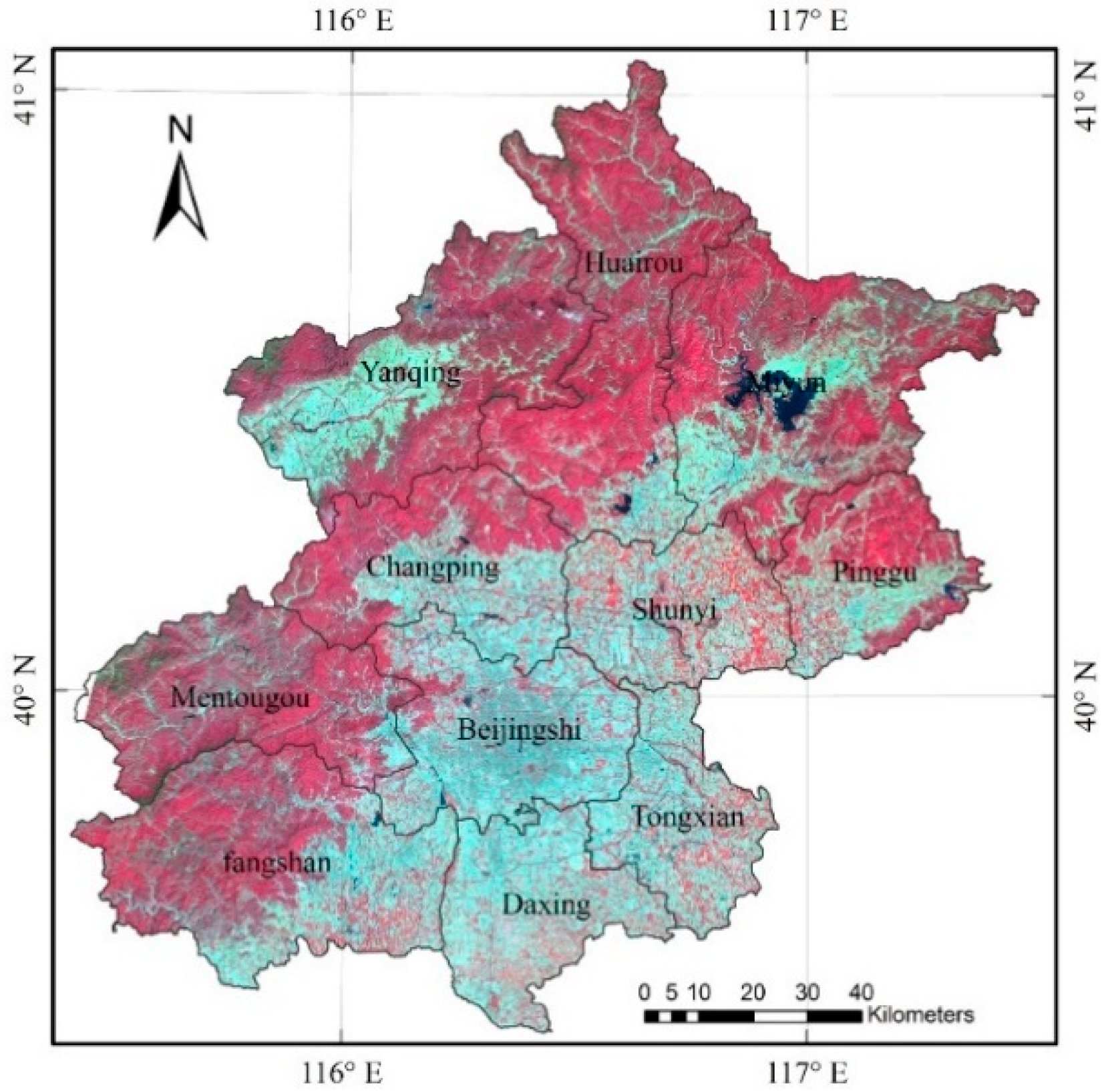
Beijing covers an area of approximately 16,800 km², from latitude 39°26'N to 41°03'N and from longitude 115°25'E to 117°30'E (Figure 1). The city is located in the north of the Northern China Plain, and belongs to the temperate climatic zone, which has an average annual temperature of approximately 12 °C and an average annual precipitation of approximately 664 mm. The geography of Beijing is characterized by alluvial plains in the south and east, whereas hills and mountains dominate the northern, northwestern, and western regions. The diverse land cover types that occur in the area, including forest, grass, cropland, urban regions, and water, make land cover classification in Beijing a suitable focus for this study.

The Landsat dataset was one of the most valuable datasets for understanding the global land cover status and freely provided by the United States Geological Survey (USGS) over the Internet [27]. In this study, two Landsat 8 [28,29] Operational Land Imager (OLI) images covering the study area (path/row: 123/32 and 123/33), were downloaded from the USGS website [30]. The OLI data were mostly not affected by cloud and the quality of the multispectral data was good (Figure 1). The OLI data were atmospherically corrected using FLAASH tools provided by ENVI version 5.0 to convert the DN value of the raw data to surface spectral reflectance. In the FLAASH tools, the atmospheric model, aerosol model, aerosol retrieval, and initial visibility were set to Sub-Arctic Summer, Urban, 2-band (K-T), and 40 km, respectively. Finally, the mosaic and subset tools were used to extract the surface spectral reflectance of OLI data to cover the study area.

Figure 1. The location of the study area and the Landsat OLI data acquired on 12 May 2013 (presented in false color image: R = NIR, G = red, B = green).

Figure 1. The location of the study area and the Landsat OLI data acquired on 12 May 2013 (presented in false color image: R = NIR, G = red, B = green).

MODIS 16-day composited NDVI data (MOD13Q1, L3 Global 250 m version 5) in HDF format covering the study area from October 2012 to September 2013 were acquired from the National Aeronautics and Space Administration (NASA) of the United States Warehouse Inventory Search Tool. MOD13Q1 provides data every 16 days at a spatial resolution of 250 m in a sinusoidal projection. The Savitzky-Golay (S-G) filter was used to smooth the time series MODIS NDVI data, specifically for removing the noise caused primarily by cloud contamination and atmospheric variability [31,32]. The smoothed MODIS NDVI data were reprojected to the same projection with OLI data, and the spatial resolution was resampled to 30 m. Finally, the same columns and lines of MODIS NDVI data were extracted to maintain consistency with OLI data for further analysis.

3. Methods

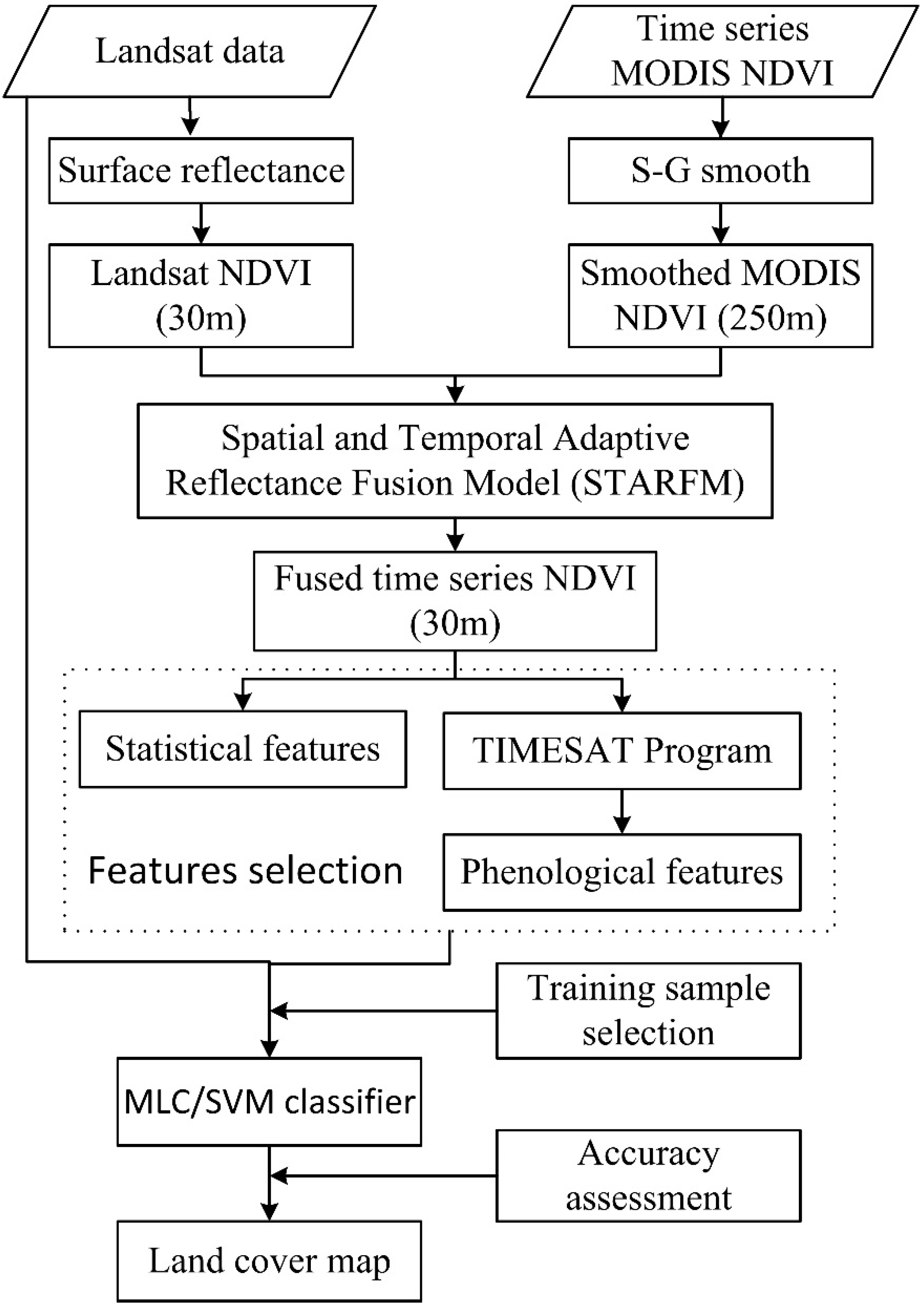
The flowchart of this study is presented in Figure 2. First, the time series MODIS NDVI data were fused with NDVI derived from OLI data using the Spatial and Temporal Adaptive Reflectance Fusion Model (STARFM) [33]. Statistical temporal features were calculated and phenological features were extracted from the fused time series NDVI data using the TIMESAT toolbox, a well-established program for extracting the seasonality of satellite time series data [20,21]. Finally, the phenological features and the statistical temporal features combined with OLI spectral bands were used for land cover classification with supervised classifiers, and an accuracy assessment was conducted to investigate whether the phenological features could significantly improve the land cover classification accuracy of Landsat data.

3.1. Fusion of Time Series MODIS NDVI and OLI NDVI Data

STARFM was selected to fuse high temporal resolution information from MODIS NDVI data and high spatial resolution information from Landsat OLI data. STARFM predicts pixel values based on the spatially weighted difference computed between the Landsat and the MODIS NDVI data acquired at T1 and one or more MODIS scenes of the prediction day (T2), respectively [33]. Ideally, in the fusion process, if Landsat data from multiple dates are being used, one would expect higher fidelity for the predicted finer resolution NDVI data using the MODIS NDVI and STARFM methods. However, only one cloudless Landsat 8 OLI data of high quality was acquired in this study, further illustrating the difficulty in obtaining time series high spatial resolution remote sensing data. Thus, it was hypothesized that land cover types did not change in the Landsat image across the temporal MODIS NDVI data. Land cover types generally change little over one year. Therefore, the spatially weighted difference in the STARFM method should not be changed significantly using the single Landsat data in the fusion process, and the predicted time series NDVI data could reflect the actual change trend of NDVI.

Figure 2. The flowchart of land cover classification of Landsat data with phenological features extracted from time series MODIS NDVI data.

Figure 2. The flowchart of land cover classification of Landsat data with phenological features extracted from time series MODIS NDVI data.

In this study, the OLI NDVI data were scaled to 0–10,000 and designated the Landsat T1-scene data. The same scaled and spatially resampled (30 m) MODIS NDVI data (acquired on Julian day 129 of 2013) that were nearest to the OLI data were designated the MODIS T1 data. The time series MODIS NDVI data acquired from October 2012 to September 2013 were then scaled to 0–10,000 and used to produce Landsat-like NDVI data. Finally, fused NDVI time series data gathered over a 16-day interval at a spatial resolution of 30 m were generated for further analysis.

3.2. Phenological Features Extraction

Phenological features were obtained using the TIMESAT toolbox. Because one year of fused NDVI time series data were gathered and the vegetation season peaks were near the middle of the time series, for this study the time series data could be duplicated to produce an artificial time series spanning three years to extract the seasonality parameters using the TIMESAT toolbox [20]. In the TIMESAT toolbox, the NDVI time series data were first fitted to a double-logistic function, and then phenological features were extracted [20,21]. The extraction of phenological features over one year of NDVI time series data was recommended to improve land cover classification accuracy because one year of data would better reflect the actual phenological features in the study period. Data gathered over a greater number of years may cause confusion in phenological features extraction; for example, cropland may be fallow in one year, or crop types may vary between different years. Such variations could lead to changes in phenological features. The phenological features extracted for improving land cover classification accuracy in this study included the beginning and ending dates of the growing season, the length of the growing season, the seasonal amplitude, and the maximum fitted NDVI value. The beginning and ending dates of the growing season were defined as the times at which the fitted NDVI curve reached 50% of the seasonal amplitude measured from the left and right minimum values, respectively. More information about the definition of the phenological features used in this study can be found in [20]. To compare the classification results obtained using phenological features, four statistical temporal features of the time series fused NDVI data—the maximum, minimum, mean, and standard deviation values—were also extracted for land cover classification.

3.3. Supervised Classifiers

The widely used maximum likelihood classifier (MLC) and SVM classifier were selected for land cover classification in this study [34,35,36]. The SVM classifier is the most widely used advanced non-parametric statistical learning classifier, usually performing well in land cover classification studies [37,38]. Because the coastal aerosol and blue bands of OLI data are significantly correlated and the coastal aerosol band is mainly designed for monitoring coastal waters and aerosol levels, the coastal aerosol band was removed from the input variables of the supervised classifiers. Similarly, the cirrus band was also removed from the classification because it was designed for cloud identification and contained limited land surface information. Finally, bands 2, 3, 4, 5, 6, and 7 of the OLI data and the composite OLI spectral bands with phenology features and statistical temporal features were separately used for land cover classification with the MLC and SVM classifiers to investigate the efficacy of phenological features and non-parametric classifiers on improving classification accuracy.

Based on the knowledge of land cover type distribution in the study area, six classes—water, crop, bare land, impervious, grass, and forest—were identified as the final classification categories. Samples (Table 1) were randomly selected from known areas using the “region of interest” (ROI) tools provided by ENVI version 5.0 software, with the help of the researchers’ experiential knowledge on the actual distribution of land cover types and their characteristics presented in remote sensing images. The Google Earth tool was also employed to help identify land cover types. Half of the sample pixels were randomly selected as training samples, and the remaining half were selected as validating samples.

Table 1. Number of ROIs and pixels used for training and validating the classifiers.

Sample Types	Water	Crop	Bare Land	Impervious	Forest	Grass
Number of ROIs	22	86	51	33	107	81
Number of pixels	6046	6860	7922	7046	13,390	4730

Table 1. Number of ROIs and pixels used for training and validating the classifiers.

Sample Types	Water	Crop	Bare Land	Impervious	Forest	Grass
Number of ROIs	22	86	51	33	107	81
Number of pixels	6046	6860	7922	7046	13,390	4730

3.4. Classification Accuracy Assessment

The classification accuracy of the MLC and SVM classifiers using only OLI spectral data, OLI spectral data integrating phenological features, and OLI spectral data integrating statistical temporal features were assessed via quantitative classification accuracy indicators, including overall classification accuracy, producer’s accuracy, user’s accuracy, and Kappa statistics [39,40,41,42]. The reference data used to support the accuracy assessment consisted of randomly selected samples that included 3023 pixels for water, 3430 pixels for crop, 3961 pixels for bare land, 3523 pixels for impervious, 6695 pixels for forest, and 2365 pixels for grass. Furthermore, a Z-test was performed to assess significant differences between the accuracy measurements of different classification results [40]. The Z-test is a statistical test of the difference in accuracy values; it involves comparing the accuracy of a new classifier against one derived from the application of a standard classifier. Because one of the most widely used means of comparing classification accuracy in remote sensing is the comparison of kappa coefficients, the statistical significance of the difference between two independent kappa coefficients derived from different classifications is evaluated by calculating the Z-test value:

$$\text{z}=\frac{{\widehat{k}}_1-{\widehat{k}}_2}{\sqrt{{\widehat{\sigma }}_{k_1}^2+{\widehat{\sigma }}_{k_2}^2}}$$

(1)

where ${\widehat{k}}_1$ and ${\widehat{k}}_2$ represent the estimated kappa coefficients for the classification derived from two different classifications, and ${\widehat{\sigma }}_{k_1}^2$ and ${\widehat{\sigma }}_{k_2}^2$ represent the corresponding variances [40]. Assuming a normal distribution, a difference is considered to be statistically significant if |z| > z_α/2, where z_α/2 represents the value cutting off the proportion α/2 in the standard normal curve’s upper tail and can be determined from statistical tables. Thus, if α = 0.05 the Z-test will yield z > 1.96 or z < −1.96; the difference can be declared significant at the 5% significance level. Therefore, |z| > 1.96 will indicate that the two compared classifications are significantly different at the 5% significance level.

4. Results and Discussions

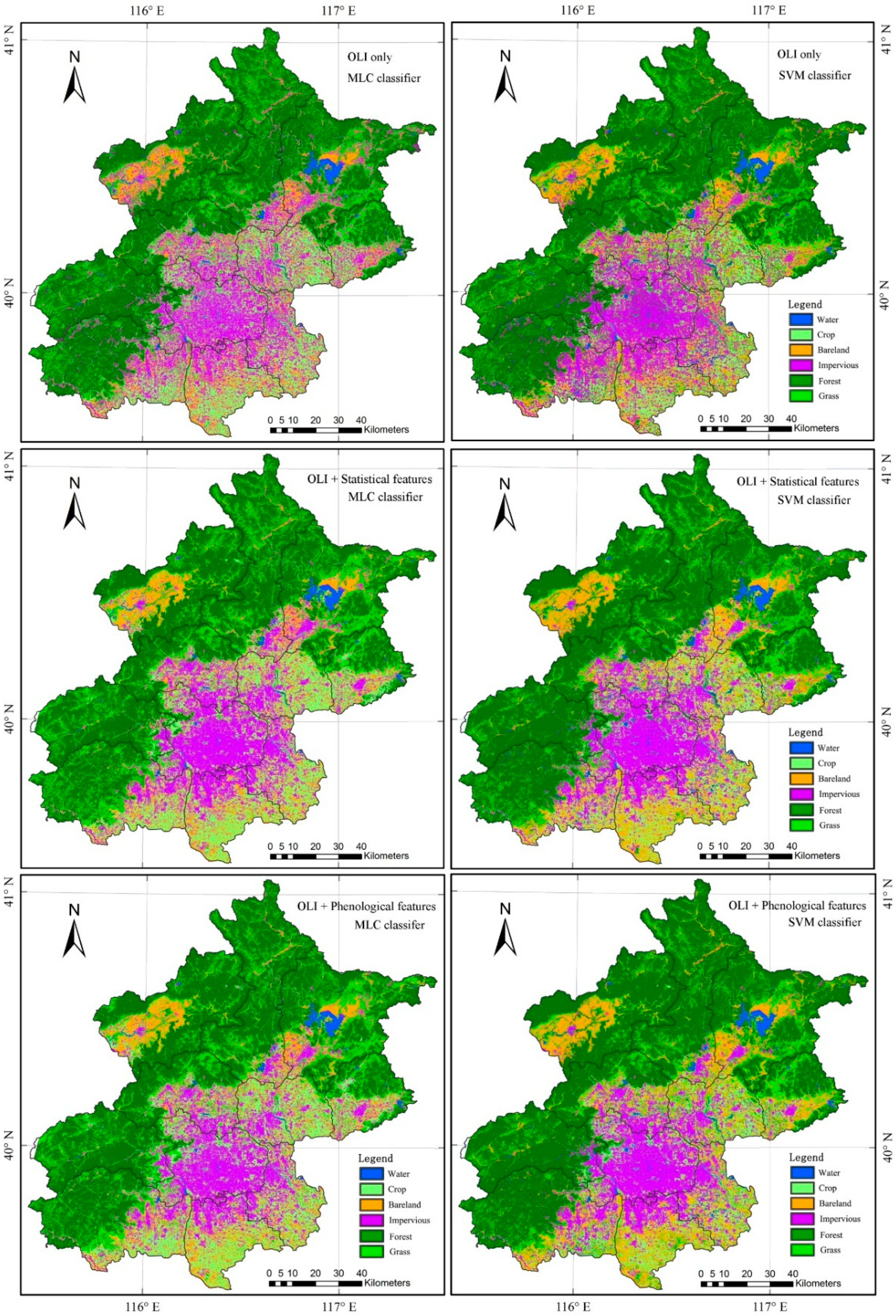
The land cover classification results (Figure 3) show that spatial distribution of land cover types is consistently achieved using MLC and SVM classifiers with only OLI spectral data, the OLI spectral data integrated with phenological features and statistical temporal features extracted from time series MODIS NDVI data. The distribution of forests, crops, bare land, water, and impervious surfaces reflects the actual land cover situation in the study area, based on visual observation and experts’ knowledge. Forests and grasses are mainly distributed in the northern, northwestern, and western mountain regions, whereas the impervious surfaces are primarily distributed in urban regions. Preliminary observation shows that the classification results for different configurations are reasonable. The main improvement achieved by using phenological features or statistical temporal features was that vegetation types could be more effectively identified. Regarding different classifiers, the SVM classifier performed slightly better than the MLC classifier.

Figure 3. Land cover classification results of MLC and SVM classifiers with different configurations.

Figure 3. Land cover classification results of MLC and SVM classifiers with different configurations.

The confusion matrices and kappa statistics for quantitatively assessing the performance of land cover classification results of the MLC and SVM classifiers using only OLI spectral data, combined OLI spectral data with phenological features, and statistical temporal features were calculated using the validation samples. Overall classification accuracies, producer’s and user’s accuracies, and kappa coefficients are presented in Table 2. The land cover classification performances were all satisfactory. OLI spectral data integrating phenological features achieved better classification accuracy using both the MLC (overall accuracy: 93.5%; kappa coefficient: 0.920) and SVM (overall accuracy: 93.8%; kappa coefficient: 0.924) classifiers than the classification result for only OLI spectral data using the MLC (overall accuracy: 90.4%; kappa coefficient: 0.881) and SVM (overall accuracy: 91.3%; kappa coefficient: 0.893) classifiers. These findings were similar to those obtained by visual observation.

The five phenological features extracted from time series fused NDVI data improved the overall classification accuracy by approximately 3% and the kappa coefficient value by approximately 3% compared to that obtained by using only OLI spectral data (Table 2). User’s accuracy and producer’s accuracy for almost all land cover types improved when using phenological features, especially for grass, which showed an accuracy improvement of more than 10%. These results further indicate that phenological features contain important information for land cover classification when using remote sensing data, especially for vegetation type discrimination because different vegetation types usually have separable phenological features that can be captured by time series vegetation index profiles. The phenological features extracted using the TIMESAT toolbox contained vegetation growing characteristic information and could weaken the effect of cloud, terrain, and shadow on the land cover classification of single Landsat OLI data, thus significantly improving the classification accuracy, especially for vegetation type classification.

Table 2. Classification accuracies for MLC and SVM classifiers with different configurations (%).

Land Cover Types	Accuracy Types	OLI Spectral Data		OLI+ Statistical Features		OLI+ Phenological Features
		OLI_MLC *	OLI_SVM	Stat_MLC	Stat_SVM	Phen_MLC	Phen_SVM
Water	Pro. Acc.	96.8	99.3	97.0	99.6	96.9	99.5
	User Acc.	100.0	99.3	100.0	99.9	100.0	99.9
Crop	Pro. Acc.	92.5	96.1	96.5	98.0	94.4	95.7
	User Acc.	91.8	95.9	94.8	96.3	91.4	94.8
Forest	Pro. Acc.	91.4	91.9	93.5	93.9	92.6	92.2
	User Acc.	87.0	87.5	93.4	92.8	92.9	91.9
Impervious	Pro. Acc.	91.5	92.6	96.4	97.2	93.6	97.1
	User Acc.	93.0	94.2	95.7	97.6	93.6	96.8
Bare land	Pro. Acc.	96.9	95.3	98.3	97.9	98.2	97.3
	User Acc.	93.6	94.2	96.8	97.5	98.2	97.1
Grass	Pro. Acc.	63.6	63.8	83.4	81.4	82.7	78.1
	User Acc.	74.8	74.3	85.6	86.3	85.8	79.9
Overall classification accuracy		90.4	91.3	94.6	95.2	93.5	93.8
Kappa Coefficient		0.881	0.893	0.934	0.941	0.920	0.924

* Note: OLI_MLC represented the result of the MLC classifier obtained using OLI spectral data; other symbols were similar and represented classification results obtained using different configurations. Stat: statistical temporal features integrated with OLI spectral data. Phen: phenological features integrated with OLI spectral data. Pro. Acc.: Producer’s Accuracy. User Acc.: User’s Accuracy.

Table 2. Classification accuracies for MLC and SVM classifiers with different configurations (%).

Land Cover Types	Accuracy Types	OLI Spectral Data		OLI+ Statistical Features		OLI+ Phenological Features
		OLI_MLC *	OLI_SVM	Stat_MLC	Stat_SVM	Phen_MLC	Phen_SVM
Water	Pro. Acc.	96.8	99.3	97.0	99.6	96.9	99.5
	User Acc.	100.0	99.3	100.0	99.9	100.0	99.9
Crop	Pro. Acc.	92.5	96.1	96.5	98.0	94.4	95.7
	User Acc.	91.8	95.9	94.8	96.3	91.4	94.8
Forest	Pro. Acc.	91.4	91.9	93.5	93.9	92.6	92.2
	User Acc.	87.0	87.5	93.4	92.8	92.9	91.9
Impervious	Pro. Acc.	91.5	92.6	96.4	97.2	93.6	97.1
	User Acc.	93.0	94.2	95.7	97.6	93.6	96.8
Bare land	Pro. Acc.	96.9	95.3	98.3	97.9	98.2	97.3
	User Acc.	93.6	94.2	96.8	97.5	98.2	97.1
Grass	Pro. Acc.	63.6	63.8	83.4	81.4	82.7	78.1
	User Acc.	74.8	74.3	85.6	86.3	85.8	79.9
Overall classification accuracy		90.4	91.3	94.6	95.2	93.5	93.8
Kappa Coefficient		0.881	0.893	0.934	0.941	0.920	0.924

* Note: OLI_MLC represented the result of the MLC classifier obtained using OLI spectral data; other symbols were similar and represented classification results obtained using different configurations. Stat: statistical temporal features integrated with OLI spectral data. Phen: phenological features integrated with OLI spectral data. Pro. Acc.: Producer’s Accuracy. User Acc.: User’s Accuracy.

However, when considering the performance of different temporal-related features used for land cover classification, the phenological features using both the MLC (overall accuracy: 93.5%; kappa coefficient: 0.920) and SVM (overall accuracy: 93.8%; kappa coefficient: 0.924) classifiers did not improve on statistical temporal features using the MLC (overall accuracy: 94.6%; kappa coefficient: 0.934) and SVM (overall accuracy: 95.2%; kappa coefficient: 0.941) classifiers (Table 2). Taking the results of the MLC classifier as an example, the main difference in the individual land cover type discrimination accuracies of phenological features and statistical temporal features occurred in the crop category. Producer’s and user’s accuracies for crops achieved using statistical temporal features were approximately three percentage points higher than those obtained by using phenological features. A similar phenomenon was observed in the classification accuracy of impervious surfaces. For other land cover types, however, the classification accuracies showed few differences. These results may have been caused by the fact that crops area human-managed vegetation type, and the planting time for different fields may be different, thus leading to different crop fields having differences in phenological characteristics. Another reason is that the harvest time for different crop fields may also show large differences, thus leading to the difference in extracted phenological features. However, the statistical temporal features are the basic statistical values of annual NDVI, which are not sensitive to crop planting and harvest times. Therefore, the statistical temporal features could better reflect crop growth characteristics and yield better classification results than phenological features could. With respect to the natural vegetation types (forest and grass), the performance of phenological features was similar to that of statistical temporal features, indicating that both phenological features and statistical temporal features could capture the growth characteristics of natural vegetation types. Therefore, it was understandable that the overall performance of phenological features did not improve on basic statistical temporal features, although the phenological features were also suitable for improving land cover classification accuracy.

Regarding the results obtained using the different classifiers applied in this study, the SVM classifier performed slightly better than the MLC classifier, and the overall improvement in accuracy was approximately one percentage point (Table 2). These findings indicate that an advanced non-parametric classifier could achieve a more satisfactory classification result than the classical MLC classifier. Similarly, considering the discrimination accuracy of individual land cover types, the accuracy improvement afforded by the SVM classifier for the crop category was more distinct than the improvements in other categories. In addition, based on visual observation of the classification results, the SVM classifier tended to yield more aggregated class objects, and fragmentized patches were reduced. Because crop fields were usually presented in regular land parcels, the SVM classifier was more beneficial in improving the classification accuracy of croplands. Unfortunately, grasslands co-existed with forest and showed smaller areas in the forest gaps and boundaries; therefore, the aggregated effect of the SVM classifier might lead to lower classification accuracy for grasslands and, lead to the misclassification of grasslands and forest lands. Therefore, the SVM classifier achieved a more distinct accuracy improvement for cropland than the MLC classifier, whereas the improvement for other land cover types was not clear. These results also indicate that the SVM classifier was more suitable in improving the classification accuracy of land cover types presented in aggregated fields.

A Z-test was used to compare the confusion matrices to determine whether the classification accuracies achieved for different configurations were significantly different (Table 3). In this context, if the two compared error matrices were not significantly different, when given the choice of only these two approaches, one should use the easier, quicker, or more efficient approach; accuracy would not be the deciding factor for choosing a classification strategy in this situation. |z| > 1.96 would indicate that the difference between two confusion matrices was significant at the 5% significance level [40]. The Z-test values for all of the different configurations were greater than 1.96, except for the comparison between the classification results using the MLC and SVM classifiers based on phenological features. These results indicate that both the phenological features and statistical temporal features could significantly improve the land cover classification accuracy of single Landsat OLI spectral data. The classification accuracy obtained by using the MLC and SVM classifiers based on phenological features was not significantly different. Additionally, the difference between the results yielded by the MLC and SVM classifiers using statistical temporal features was relatively small compared to that for the other Z-test values (Z-test value was 2.57). In contrast, the difference between the results obtained using the MLC and SVM classifiers with only Landsat OLI spectral data was greater than that obtained by integrating temporal-related information in the classification. When the amount of information used for land cover classification was smaller, the SVM classifier could achieve a much better classification result than the MLC classifier, whereas with a larger amount of information for classification, the improvement yielded by the SVM classifier decreased. All of the Z-test values for classification results yielded by using temporal-related features and only spectral features clearly showed greater values, regardless of different classifiers. These findings indicate that the classification accuracy improvement achieved by adding temporal-related information is much greater than that of a selection of complex classifiers. In other words, the use of advanced classifiers affords a smaller improvement in classification accuracy than that achieved by the approach involving additional useful features for land cover classification.

Table 3. Z-test values for comparison between confusion matrixes of land cover classification with different configurations.

Classification Methods	OLI_MLC *	OLI_SVM	Stat_MLC	Stat_SVM	Phen_MLC	Phen_SVM
OLI_MLC	-
OLI_SVM	3.45	-
Stat_MLC	17.53	14.12	-
Stat_SVM	20.02	16.64	2.57	-
Phen_MLC	12.57	9.14	5.04	7.60	-
Phen_SVM	13.84	10.41	3.76	6.32	1.28	-

* The meanings of the symbols are as given in the note to Table 2.

Table 3. Z-test values for comparison between confusion matrixes of land cover classification with different configurations.

Classification Methods	OLI_MLC *	OLI_SVM	Stat_MLC	Stat_SVM	Phen_MLC	Phen_SVM
OLI_MLC	-
OLI_SVM	3.45	-
Stat_MLC	17.53	14.12	-
Stat_SVM	20.02	16.64	2.57	-
Phen_MLC	12.57	9.14	5.04	7.60	-
Phen_SVM	13.84	10.41	3.76	6.32	1.28	-

* The meanings of the symbols are as given in the note to Table 2.

5. Conclusions

This study investigated the efficacies of phenological features and advanced non-parametric classifiers on improving the land cover classification accuracy of Landsat data integrating time series MODIS NDVI data. The following conclusions were drawn: (1) Phenological features extracted from time series fused NDVI data using the TIMESAT tool could significantly improve overall classification accuracy by approximately 3% compared to that achieved using only a single temporal Landsat data. The classification accuracy for almost all the land cover types improved greatly, especially for vegetation types. However, the phenological features did not improve on the basic statistical features very much. In particular, phenological features clearly showed suboptimal efficiency in improving the classification accuracy of human-managed vegetation types compared to statistical temporal features. (2) An SVM classifier could achieve better classification accuracy than the traditional MLC classifier, but the improvement in classification accuracy achieved by using advanced classifiers was inferior to that obtained using temporal-related features for land cover classification. In other words, involving more temporal-related features in land cover classification was a much better strategy than selecting advanced classifiers.