Object-Based Analysis of Airborne LiDAR Data for Building Change Detection

Abstract

Building change detection is useful for land management, disaster assessment, illegal building identification, urban growth monitoring, and geographic information database updating. This study proposes an automatic method that applies object-based analysis to multi-temporal point cloud data to detect building changes. The aim of this building change detection method is to identify areas that have changed and to obtain from-to information. In this method, the data are first preprocessed to generate two sets of digital surface models (DSMs), digital elevation models, and normalized DSMs from registered old and new point cloud data. Thereafter, on the basis of differential DSM, candidates for changed building objects are identified from the points in the smooth areas by using a connected component analysis technique. The random sample consensus fitting algorithm is then used to distinguish the true changed buildings from trees. The changed building objects are classified as “newly built”, “taller”, “demolished” or “lower” by using rule-based analysis. Finally, a test data set consisting of many buildings of different types in an 8.5 km² area is selected for the experiment. In the test data set, the method correctly detects 97.8% of buildings larger than 50 m². The accuracy of the method is 91.2%. Furthermore, to decrease the workload of subsequent manual checking of the result, the confidence index for each changed object is computed on the basis of object features.

1. Introduction

Building change detection can be used for an extensive range of applications, such as land management, disaster assessment, illegal building identification (i.e., a building that is built in violation of laws or administrative regulations), urban growth monitoring, and geographic information database updating. In developing countries, such as China and India, where many new buildings are constructed every year, methods that can rapidly and automatically detect changes in buildings are urgently needed.

Traditional building change detection usually requires a field survey or a visual inspection of multi-temporal orthophotos to identify changes in buildings. These methods are time-consuming and exhausting. In recent years, many methods have been proposed for the automatic detection of building change by using remote sensing data. These methods can be divided into four categories according to their data sources: (1) synthetic aperture radar (SAR) data, (2) high-resolution optical images, (3) height data, and (4) multiple sources of data. SAR imagery as a data source is relatively insensitive to atmospheric conditions and independent from sun illumination [1]. For example, Bovolo et al. [2] proposed a building change detection method that used two very-high-resolution SAR images to identify destroyed buildings before and after an earthquake. However, SAR imagery is also significantly affected by noise and is difficult for nonprofessionals to interpret. Previous studies [3,4,5,6,7,8] have also detected building changes by using multi-temporal very-high-resolution satellite data. The spectral information in these images is useful for separating buildings from vegetation. However, methods based on high-resolution optical images with only 2D information can suffer from spectral variation because of the degradation of building materials and the shape deformation caused by different viewpoints and building heights, shadows, and occlusions. These factors make the image-based change detection of buildings difficult. A variety of methods have used height data. Murakami et al. [9] detected changes in buildings by using a simple digital surface model (DSM) comparison of multi-temporal airborne light detection and ranging (LiDAR) data sets in urban areas. Vu et al. [10] proposed an automatic building change detection method based on LiDAR data in dense urban areas. Jung [11] provided a two-step algorithm to detect building changes by using multi-temporal aerial stereo pairs. Teo and Shih [12] used multi-temporal interpolated LiDAR data for building change detection and change-type determination in urban areas via geometric analysis. They achieved 80% accuracy. Three-dimensional surface data, which can be obtained by stereo image matching or directly from LiDAR data, provide information on building height, which is an important feature that can be effectively used as an indicator of building changes. Other researchers have combined multiple sources of data. For example, Rottensteiner [13], Hermosilla et al. [14], Grigillo et al. [15], Malpica et al. [16], and Tian et al. [17] developed automatic approaches that combined image and surface data for building change detection. Knudsen and Olsen [18], Bouziani et al. [19], and Liu et al. [20] used existing vector and spectral data as inputs for building change detection. For map database updating, Matikainen et al. [21] first combined airborne LiDAR and digital aerial images to conduct building change detection with the old map. In this method, 96% of buildings larger than 60 m² were correctly detected in the building detection step. The completeness and correctness of change detection achieved approximately 85% in a 5 km² suburban study area. Building change detection from multiple sources of data can take advantage of a variety of information. However, data registration and feature selection from different data sources should be properly handled. In many scenarios, the cost of collecting multiple data is high.

We still need to solve problems in building change detection by using height data, mainly LiDAR point clouds. First, although height difference is a major indicator of building change, other changes in height caused by vegetation (mainly trees), terrain, and noises should also be identified because these objects can significantly affect the precision of change detection. Second, the algorithm must be able to deal with an extensive range of building types in roof structure, size, and density. By contrast, existing algorithms do not consider the automatic quality assessment or self-diagnosis of the detection result; we believe that this procedure is important in improving the algorithm itself and reducing the workload of user inspection in practice. This study presents an automatic method that uses airborne LiDAR data to identify building changes in various types of buildings and to obtain from-to changes. The method attempts to solve the aforementioned issues in five steps, namely, data preprocessing, extraction of candidates for changed building objects, detection of changed building objects, determination of change type, and automatic quality assessment of the result. We focus on using object-based features to precisely extract the objects of the changed buildings. The surface smoothness of the object is used as the main feature for distinguishing buildings and trees. An object-based computation of the confidence index of each changed object is used to evaluate the quality of change detection automatically; this approach can help users check results quickly.

This paper is organized as follows: Section 2 describes the proposed method, Section 3 presents the experimental results and discussion, and Section 4 concludes.

2. Object-Based Analysis for Building Change Detection

The workflow of the proposed algorithm for building change detection is shown in Figure 1.

Figure 1. Workflow of the proposed change detection for buildings.

Figure 1. Workflow of the proposed change detection for buildings.

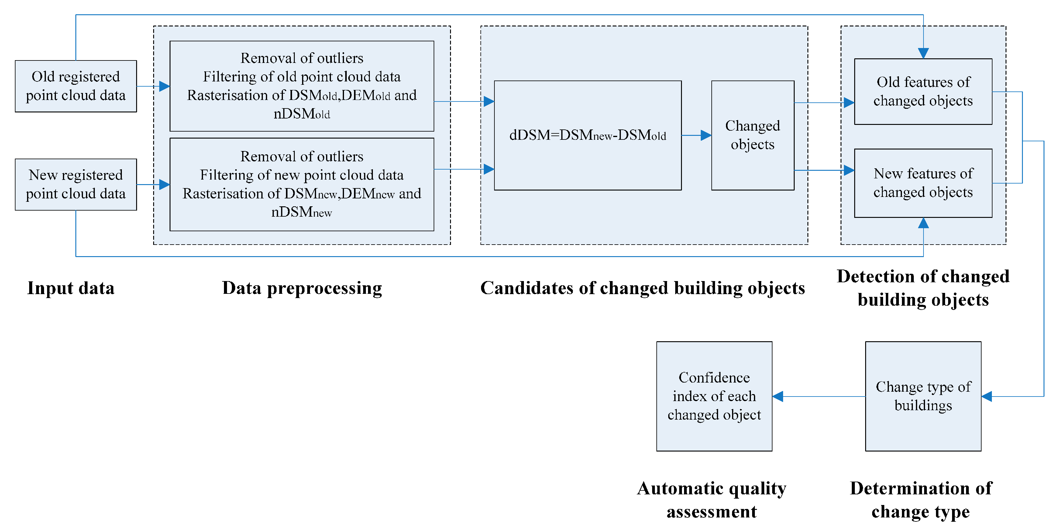
2.1. Data Preprocessing

Data preprocessing includes the removal of outliers, filtering of point cloud data, and rasterization of DSMs, digital elevation models (DEMs), and normalized DSMs (nDSMs). The details are presentedas follows:

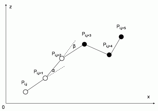
• Removal of outliers. A DEM surface interpolated by a point cloud with outliers (extremely low or high points) will be distorted and deformed. Therefore, removing outliers from old and new point clouds is necessary. In this study, the elevation histogram method [22] is first used to exclude evident outliers. The Delaunay triangulation [23,24,25] is then applied to determine the less evident outliers.
• Point cloud data filtering. Point cloud data filtering distinguishes ground points from non-ground points and has recently become a relatively mature technology. We used the commercial software TerraSolid to filter the data with the following basic principles [26,27,28]. First, a sparse triangulated irregular network (TIN) is first created from seed points. Thereafter, on the basis of the parameters derived from the data, the TIN is progressively densified in an iterative process. The iteration stops when no more points meet the thresholds.
• Rasterization of DSMs and DEMs from the old and new point cloud data. The TIN algorithm [26] is used to interpolate gridded DSMs and DEMs. By taking the generation of a new DSM as an example, the points are first arranged into a grid (the grid cell size used in this study is set to 1.0 m). Thereafter, the lowest point of each grid cell is selected to build the triangulation. Finally, the height of the gridded points of the DSM is interpolated on the basis of the three points of the located triangle. The same technique is used to acquire an old gridded DSM. A similar method is used for the rasterization of new and old DEMs, but only the ground points are used during triangulation.
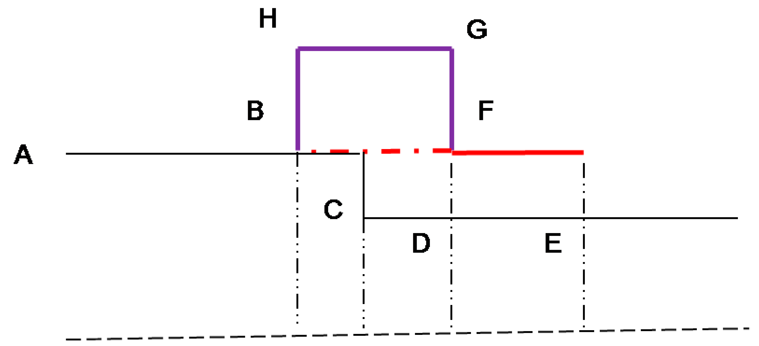
• Generation of nDSM_old and nDSM_new. nDSM is obtained by subtracting the appropriate DEM from the DSM:

  $$\text{nDS}{\text{M}}_{\text{old}} = \text{DS}{\text{M}}_{\text{old}} – \text{DE}{\text{M}}_{\text{old}},$$

  $$\text{nDS}{\text{M}}_{\text{new}} = \text{DS}{\text{M}}_{\text{new}} – \text{DE}{\text{M}}_{\text{new}}$$

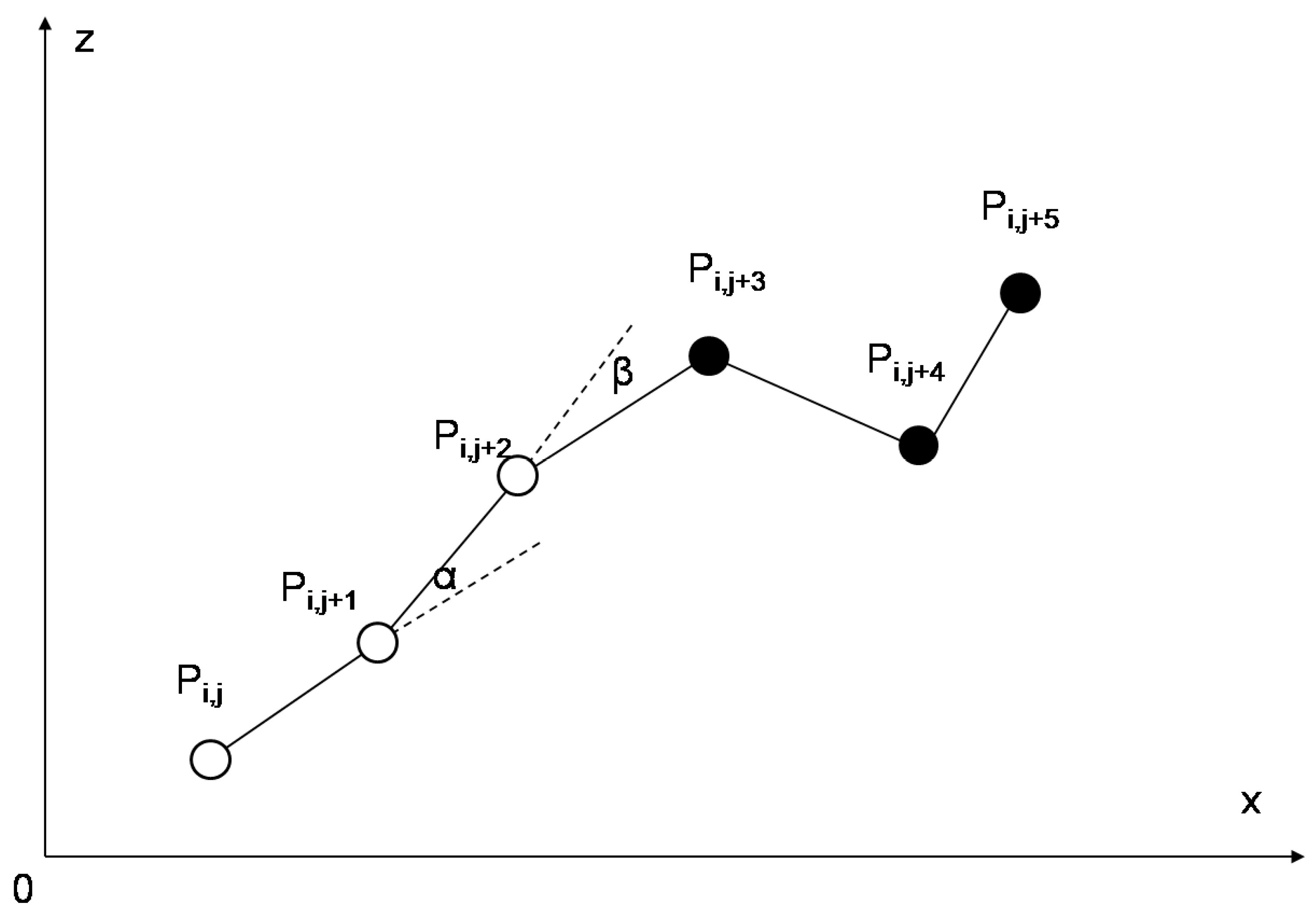
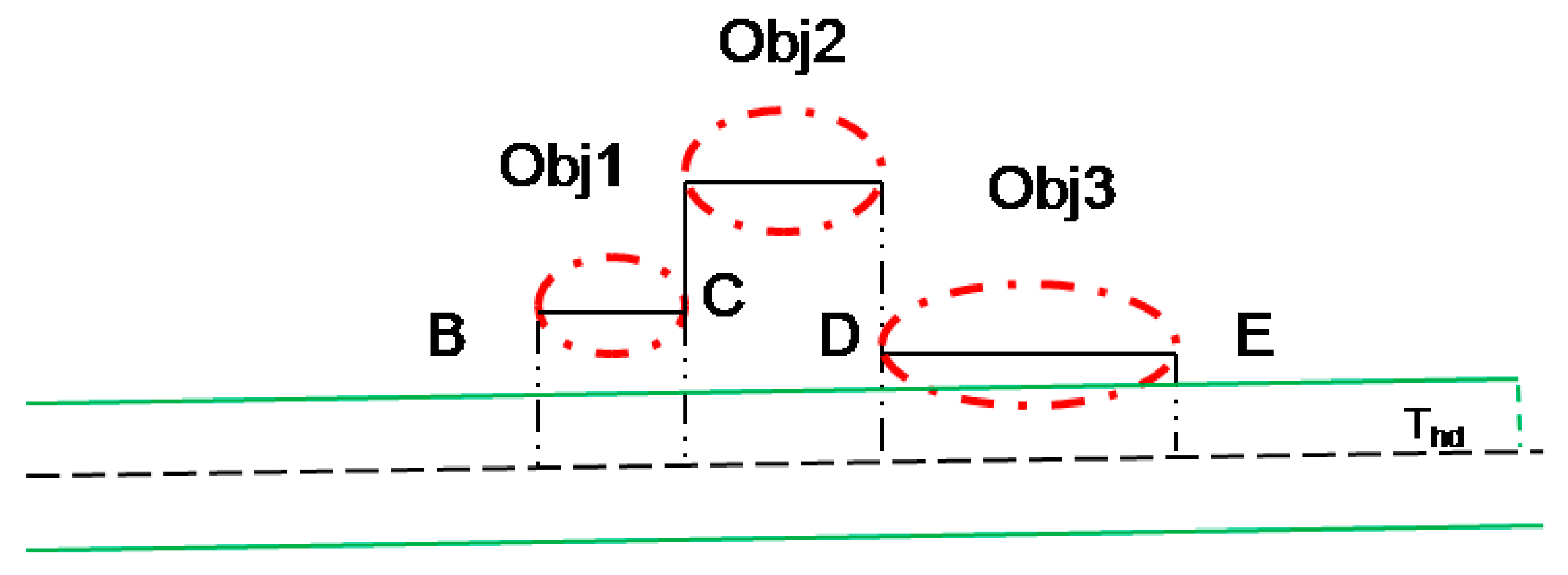
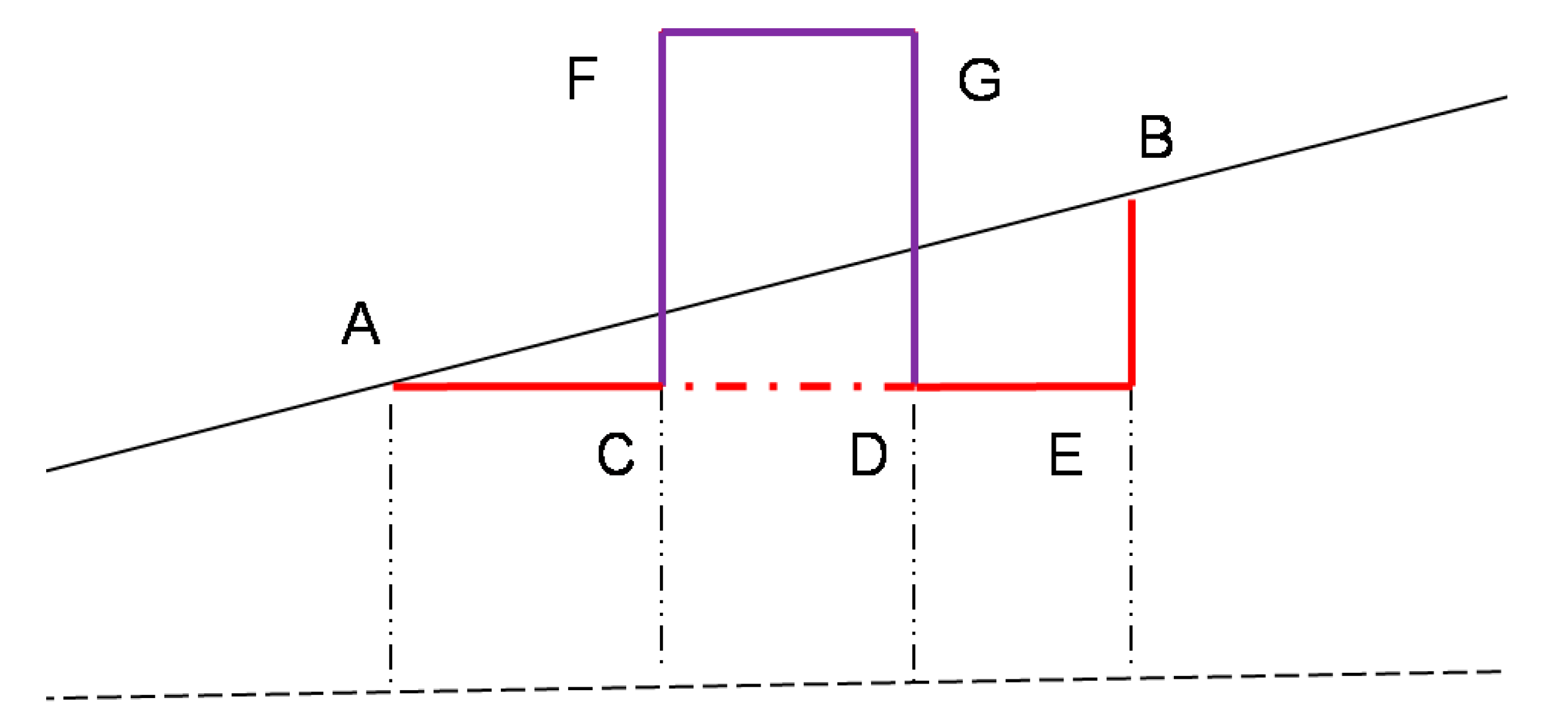
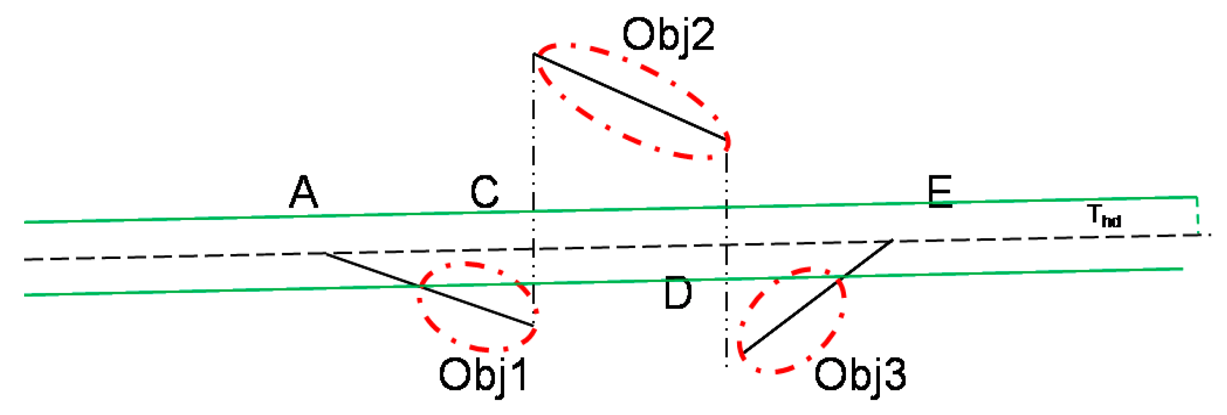
2.2. Extraction of Candidates for Changed Building Objects

In this section, candidates for changed building objects are extracted by using the differential DSM (dDSM).

First, a dDSM is obtained by subtracting DSM_old from DSM_new. The absolute height of any dDSM less than a certain elevation threshold (2.5 m) is set to 0 cm to prevent interference from trees close to the building. The presence of these points will sometimes connect the building patch to the ground, thus possibly influencing the subsequent extraction of building objects.

As building roofs usually have smooth facets, the next step is to identify the points in the smooth areas in the dDSM by using a smoothness computation. A point is classified as a smooth area point if it fulfills one of the criteria on smoothness in the row and column directions. The smoothness computation is shown in Figure 2, where P_i,j, P_i,j+1, …, P_i,j+5 are the points in the ith row or column. The white and black points represent the points of smooth and rough areas, respectively. A point (e.g., P_i,j+1) is classified as a smooth area point if angle α is less than a certain degree (in this study, 10°). Otherwise, the point is classified as a rough area point.

Figure 2. Points of smooth and rough areas (the white and black points represent the points of smooth and rough areas, respectively).

Figure 2. Points of smooth and rough areas (the white and black points represent the points of smooth and rough areas, respectively).

A connected component analysis technique is used to obtain separate objects composed of the smooth area points in the raster image. If an object is larger than a certain threshold, the object is defined as a candidate for a changed building. In this study, the threshold of the object area is set to 25 m².

2.3. Detection of Changed Building Objects

The presence of a changed building object is confirmed primarily on the basis of its planarity attribute. The roof of a building is often composed of several regular planes, whereas treetops and other non-ground objects in an original point cloud are usually irregularly distributed. Consequently, object height and planarity ratio are calculated to further distinguish true building objects from suspected building objects. The steps are as follows:

Step 1—The average height of each object is calculated by using nDSM.

Step 2—For objects with elevations greater than the threshold of the building height (in the experimental section, the threshold is set to 3.0 m), the random sample consensus (RANSAC) algorithm [29] is applied to the original point cloud data to fit the two largest planes. The model is written as Formula (1):

Ax + By + Cz + 1 = 0

(1)

where A, B, and C are the parameters of the fitting plane, and x, y, and z are the coordinates of the point. The planarity ratio r is calculated as follows:

r = (N₁ + N₂)/N_obj

(2)

where N₁ is the number of points of the largest plane fit by RANSAC, N₂ is the number of points of the second largest plane fit by RANSAC, and N_obj is the number of points of the object.

Step 3—By using a threshold of the planarity ratio t, true building objects are identified if r > t, t = 0.6.

Step 4—Repeat Steps 1 to 3 with the other periods of point cloud data.

2.4. Determination of Change Type

In this study, the change types are “newly built”, “taller”, “demolished”, and “lower”. The rules for determining the change type of buildings are as follows:

Rule1—Newly built: an object in the new point cloud is considered a building, whereas an object in the old point cloud is not.

Rule2—Taller: an object is determined to be a building in the old and new point clouds, and the height of the object in the new point cloud is greater than that in the old point cloud.

Rule3—Demolished: an object in the old point cloud is considered a building, whereas an object in the new point cloud is not.

Rule4—Lower: an object is determined to be a building in the old and new point clouds, and the height of the object in the new point cloud is smaller than that in the old point cloud.

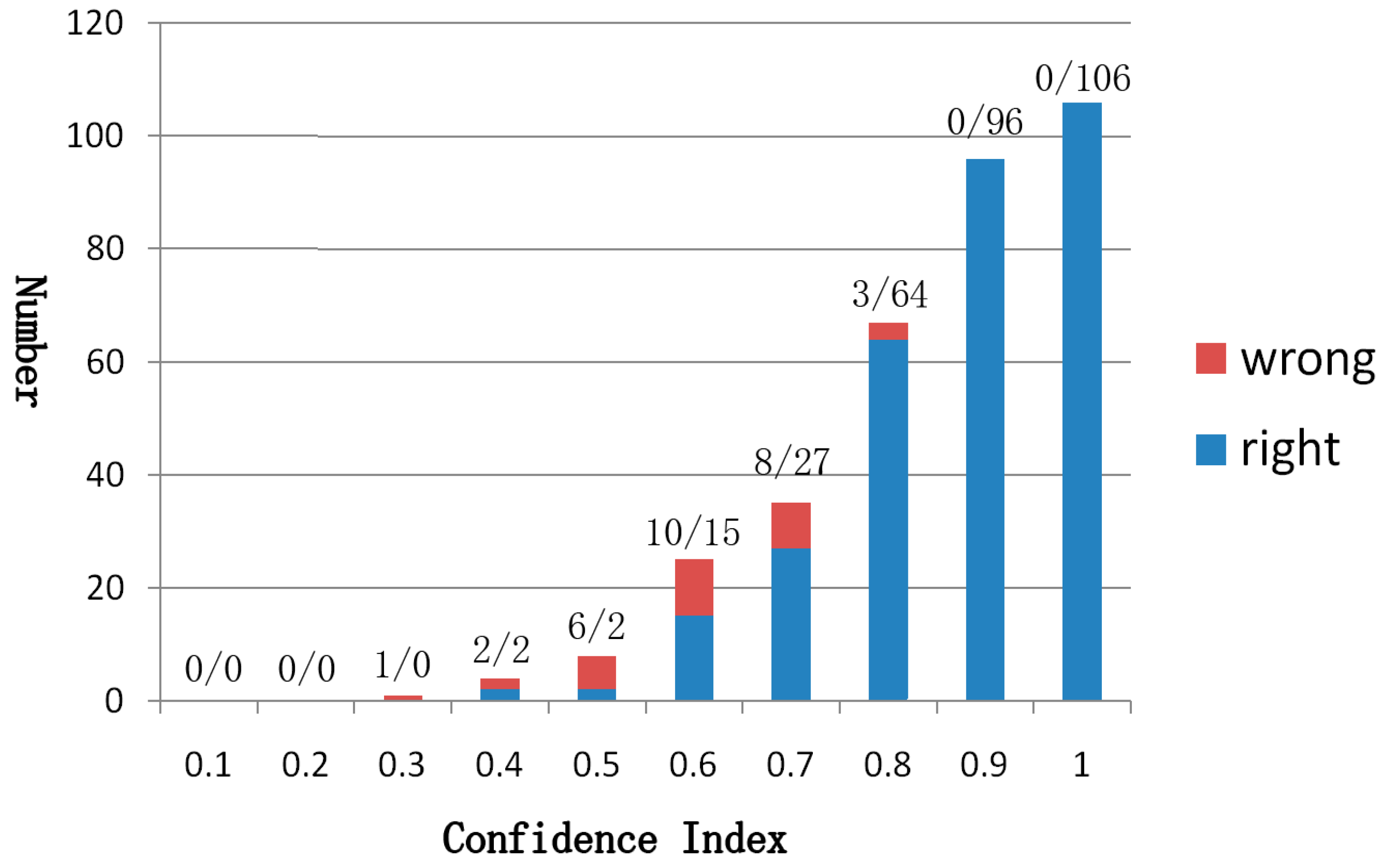
2.5. Automatic Quality Assessment of Building Change Detection

The automatic diagnosis of the result is useful for improving the performance of a feature extraction algorithm. By contrast, in the change detection practice, users have to check all detected changes carefully because of the existence of wrong detections. Wrong detections lead to time-consuming post-processing. An object-based self-diagnostic method for quality assessment is presented to improve the efficiency of inspection and the manual editing of the results. The confidence index of each changed object is computed by using the object features. The confidence index of an object is a good indicator for inspection. On the basis of the analysis of typical errors, the feature difference between the changed building objects is computed to obtain the confidence index. These features are continuity C_c, planarity C_p, and overlap C_o, which are computed as follows:

Continuity C_c: For the object that is considered a building, the largest plane is first obtained by RANSAC fitting. The region is then expanded by adding other points of the object (the distance threshold is 1.0 m). The ratio of continuity R(C) is calculated as follows:

$$\text{R}\left(C\right) = \{\begin{array}{c}\frac{A}{A_{obj}}, if obj is considered a building \\ \mathit{1.0}, if obj is not a building\end{array}$$

(3)

where A is the area of the largest plane after expanding the region, and A_obj is the area of the object. The ratios of objects in the old and new data, R(C_old) and R(C_new), are calculated and combined to obtain the continuity of each detected object: C_c = R(C_old)·R(C_new).

Planarity C_p: The planarity ratio R(P) is used to measure planarity. The planarity ratio R(P) is calculated as follows:

$$\text{R}\left(P\right) = \{\begin{array}{c}\frac{N_1 + N_2}{N_{obj}}, if obj is considered a building \\ \mathit{1.0}, if obj is not a building\end{array}$$

(4)

For the object that is considered a building, the planarity ratio R(P) is the same as Formula (2). However, for the object that is not a building and is excluded by the proposed method, the planarity ratio R(P) is equal to 1.0. This value is set to prevent the effect of the existence of objects that are not buildings in one period of the point cloud data. For each detected object, R(P_old) and R(P_new) are calculated separately and combined to obtain the planarity of each detected object: C_p = R(P_old)∙R(P_new).

Overlap C_o: If the distance between a new point and an old point is smaller than 0.2 m, these points are considered the overlap points. The ratio of the overlap is R(O) = N_overlap/N_obj, where N_overlap is the number of overlap points in the new or old point cloud and N_obj is the number of points of the object in the new or old point cloud. After calculating the new overlap ratio R(O_new) and the old overlap ratio R(O_old), the overlap property of the object is calculated as follows: C_o = MAX (R(O_old)∙R(O_new)).

Finally, the confidence index of each changed object C is obtained by combining the three types of features: C = C_c∙C_p∙(1 − C_o).

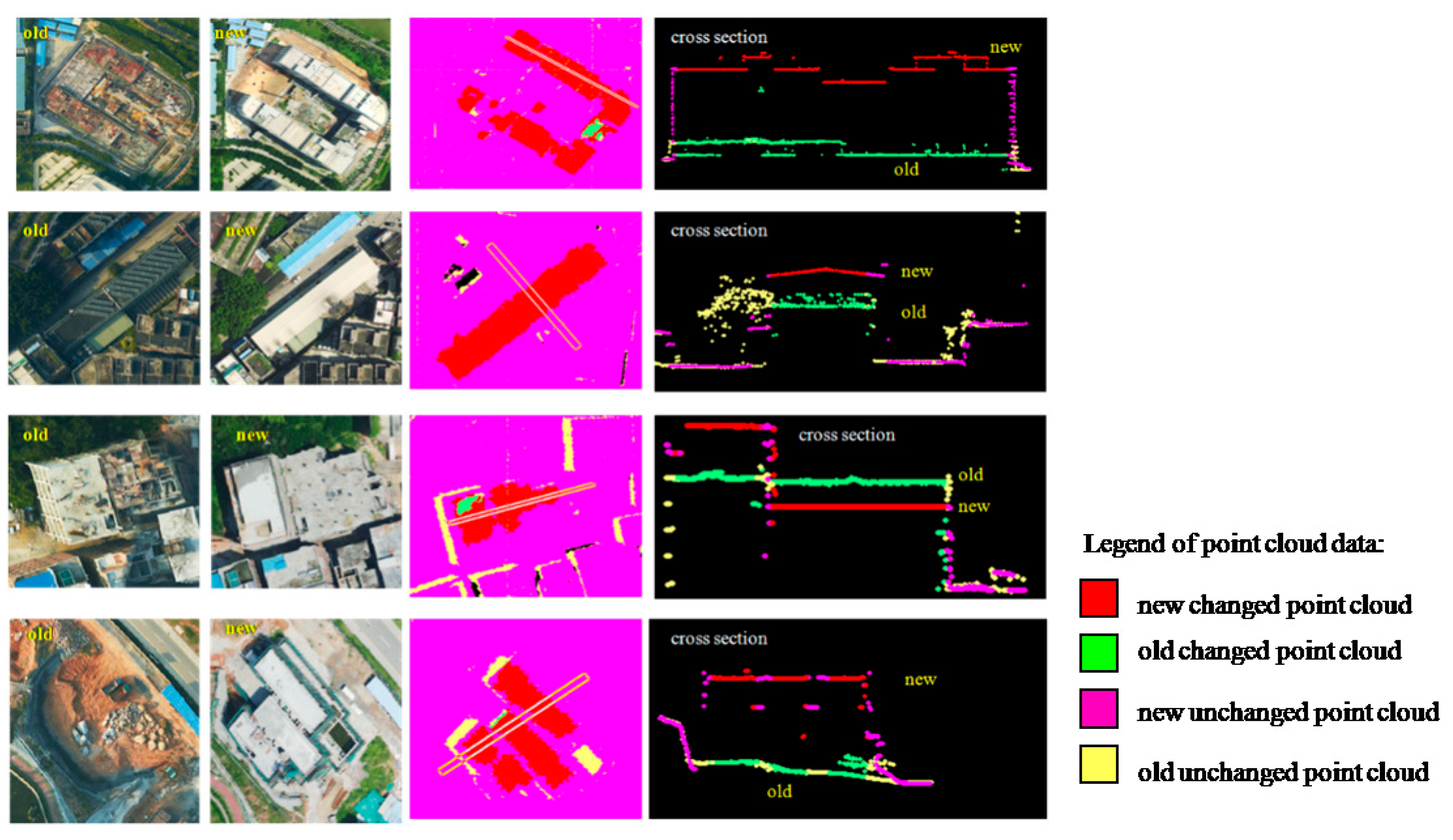
3. Experimental Results and Discussion

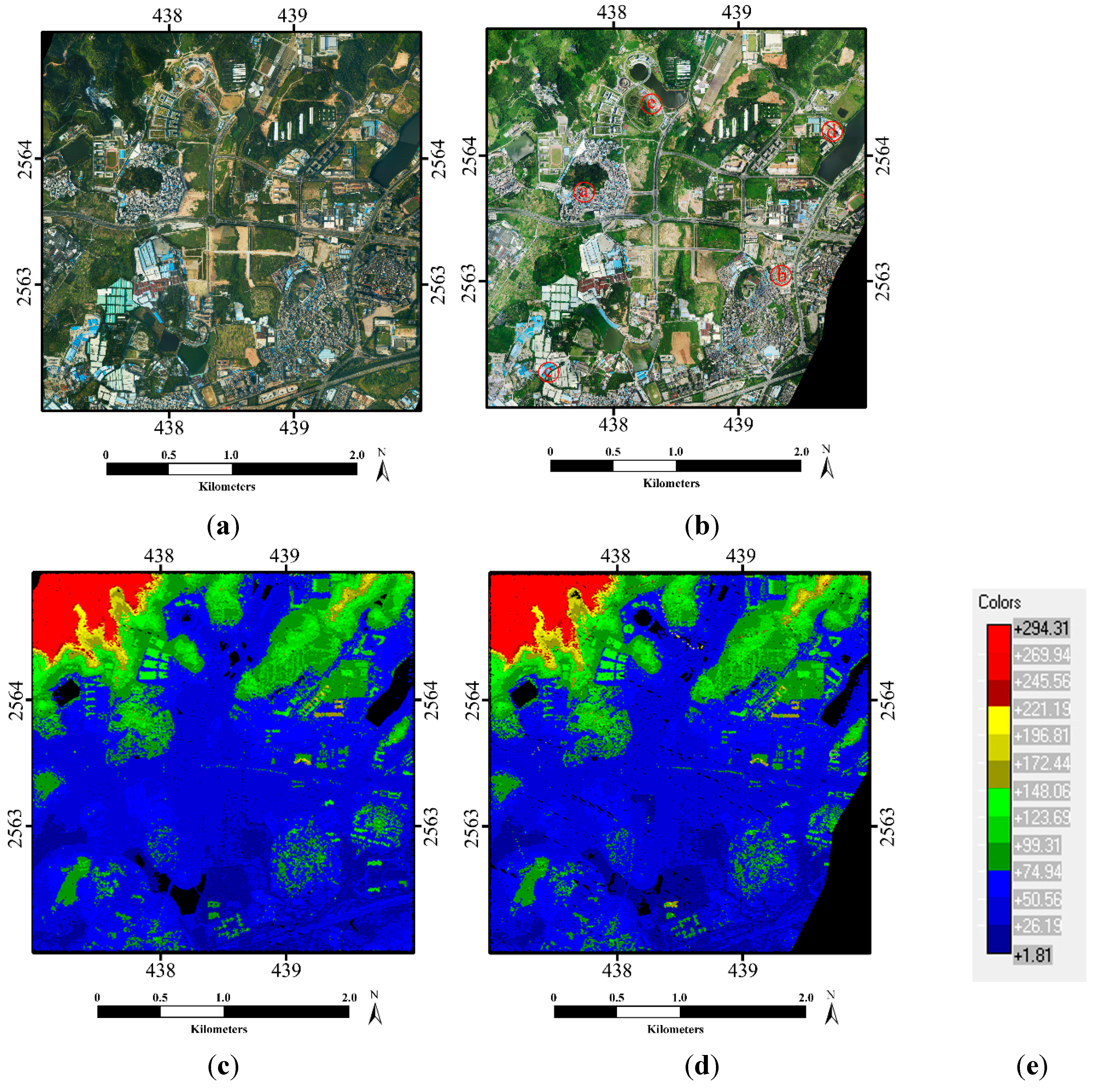
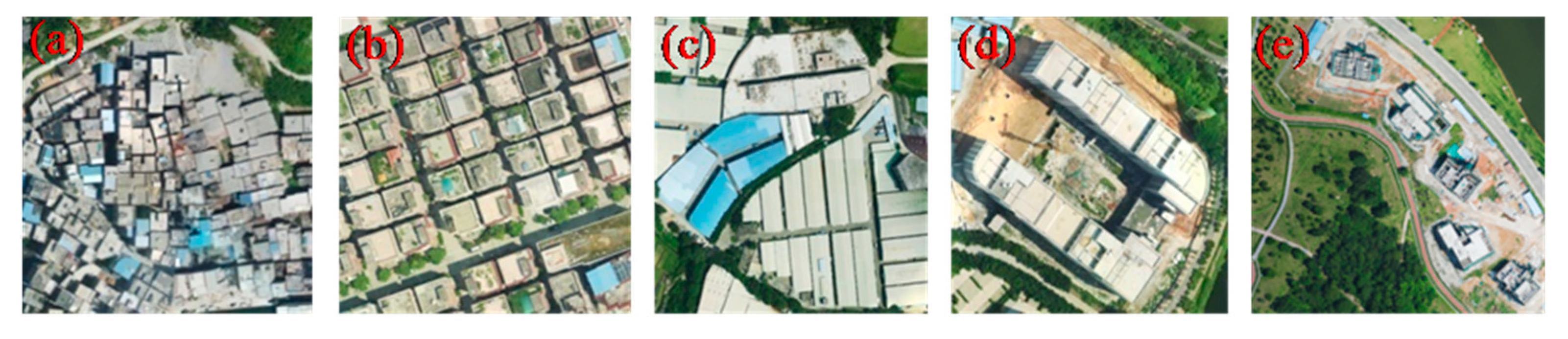
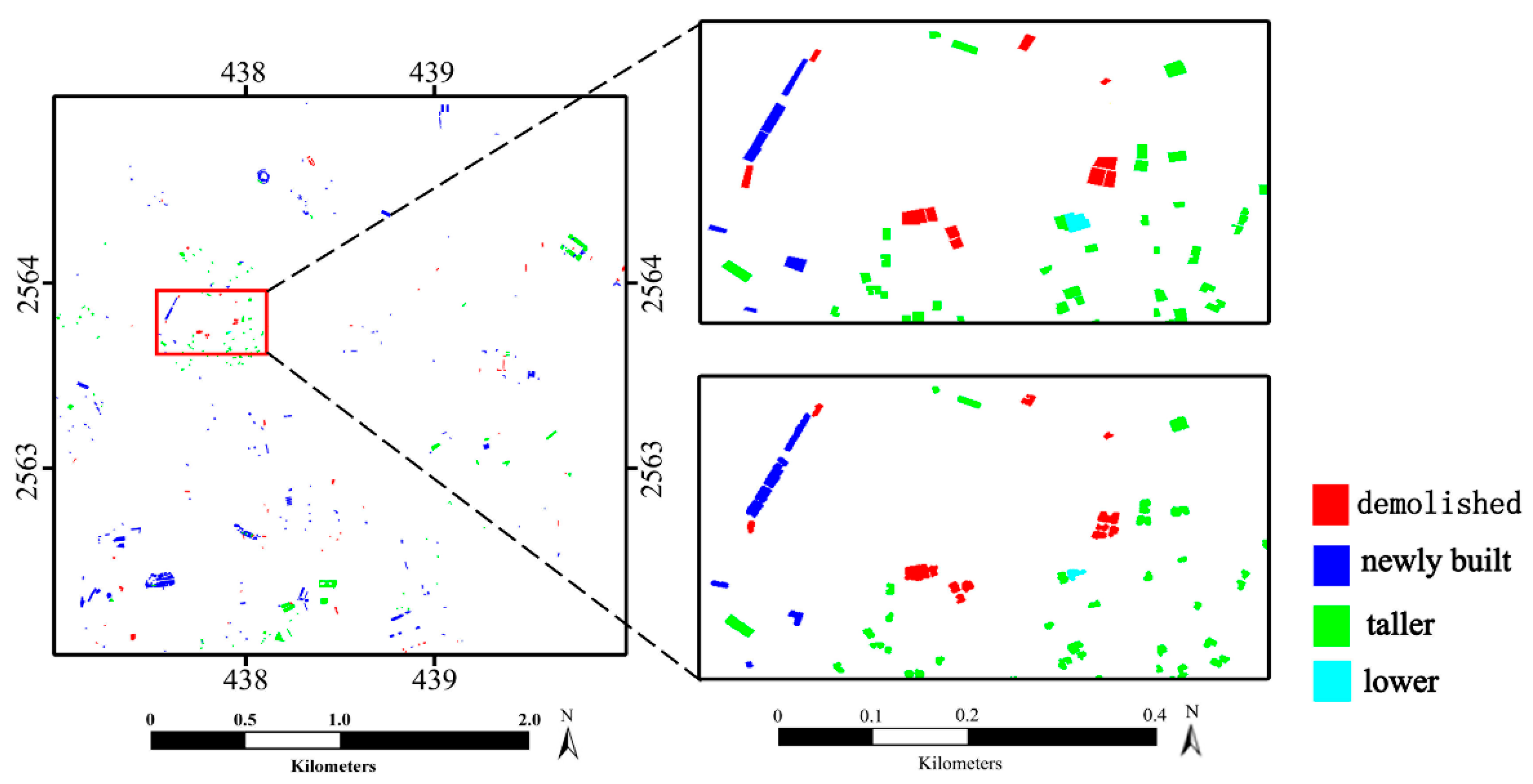
3.1. Data Set

The test site is within Guangzhou, Guangdong Province, China. Guangzhou is a modern and developing city in South China and is characterized by dense buildings with various and complex shapes in urban areas and sparse buildings and dense forests in suburbs. The area of the test data set is 9 km², but the effective overlap of the two point clouds is approximately 8.542 km². The raw data consist of two periods of point cloud data acquired by airborne LiDAR Trimble 5700 with a camera, which is able to acquire point cloud and images simultaneously. The data sets were collected in September 2011 and August 2012 separately with point densities of 4 points/m² to 6 points/m².The two data sets have been registered by iterative closest point method [30]. The corresponding aerial images acquired at the same time are not used in this study. The orthophotos with a resolution of 0.2 m are only used for visual inspection. In Figure 3d, the black area at the bottom right of the new point cloud is beyond the scan range. The other black areas are caused by the weak reflectivity of water. As observed from the orthophotos and point cloud data shown in Figure 3, the bottom part of the experimental area is a relatively flat terrain covered in dense housing with diverse structures, whereas the top part of the experimental area is a hilly terrain with sparse housing and dense forests, including a steep hill on the top left. Five details of Figure 3b, which represent the five different types of buildings in the experimental area, are shown in Figure 4.

3.2. Parameters

In the data set used in this analysis, 3000 m × 3000 m point cloud data are extremely large to process at one time. The proposed solution is to divide the data into nine nonoverlapping tiles with each tile having the size of 1000 m × 1000 m. Each tile is processed by using the same parameter set (Table 1).

Figure 3. Experimental data sets: (a) old orthophoto, (b) new orthophoto, (c) old point cloud data, (d) new point cloud data, and (e) color display index of the elevation (unit: m).

Figure 3. Experimental data sets: (a) old orthophoto, (b) new orthophoto, (c) old point cloud data, (d) new point cloud data, and (e) color display index of the elevation (unit: m).

Figure 4. Five details of Figure 3b representing the five different types of buildings in the experimental data set: (a) residential area with scattered dense buildings, (b) residential area with buildings densely aligned along the street, (c) industrial area with dense large buildings, (d) high-rise buildings, and (e) suburban area with detached buildings.

Figure 4. Five details of Figure 3b representing the five different types of buildings in the experimental data set: (a) residential area with scattered dense buildings, (b) residential area with buildings densely aligned along the street, (c) industrial area with dense large buildings, (d) high-rise buildings, and (e) suburban area with detached buildings.

Table 1. Parameterset used in the experiment.

Parameter	Threshold
Gridcell size of DSM/DEM/nDSM	1.0 m
Angle for detection of the points of smooth areas	10°
Minimum size of changed building objects	25
Minimum height of building object	3.0 m
Maximum distance from the point to the fitting plane of RANSAC	0.15 m
Minimum planarity ratio for building confirmation	0.6

Table 1. Parameterset used in the experiment.

Parameter	Threshold
Gridcell size of DSM/DEM/nDSM	1.0 m
Angle for detection of the points of smooth areas	10°
Minimum size of changed building objects	25
Minimum height of building object	3.0 m
Maximum distance from the point to the fitting plane of RANSAC	0.15 m
Minimum planarity ratio for building confirmation	0.6

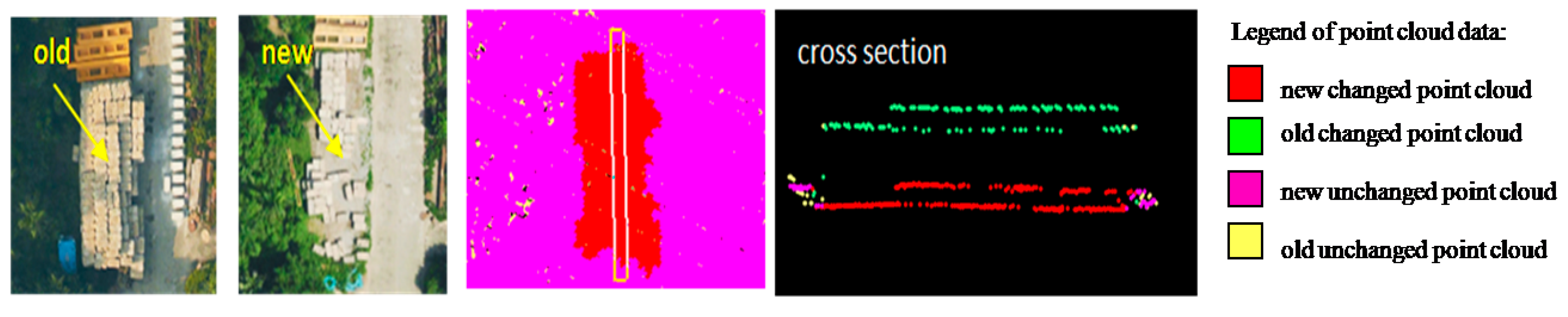
3.3. Performance

In the building change detection process, given that the area of the most important buildings is greater than 50 m², we only report the per-object completeness and correctness (Cm₅₀/Cr₅₀) of objects larger than 50 m². For the object-based metrics, as long as the object detected by the proposed method is consistent with the true change type and has some overlap with the ground truth, the object is considered to have been detected correctly. Otherwise, the object is considered to have been detected incorrectly. The per-object confusion matrix is also reported.

The ground truth, which comprises the change and change type of buildings, is obtained by the careful visual inspection of multi-temporal orthophotos and point cloud data sets. The areas of the changed buildings are manually digitized by using TerraSolid software. The details are shown on the top right part of Figure 5. The change detection results of the proposed method and part of its detail are shown on the left and bottom right of Figure 5, respectively.

Figure 5. Change detection results of the proposed method, part of the change detection result, and corresponding ground truth. Left: change detection results. Top right: details of the ground truth. Bottom right: part of the change detection result.

Figure 5. Change detection results of the proposed method, part of the change detection result, and corresponding ground truth. Left: change detection results. Top right: details of the ground truth. Bottom right: part of the change detection result.

To further validate the proposed method, examples of the change detection details are shown in Figure 6.

Figure 6. Examples of the results (first column: old orthophoto; second column: new orthophoto; third column: superposition of the old and new point clouds; fourth column: cross-section of the yellow rectangle area in the third column; fifth column: legend of the point cloud data).

Figure 6. Examples of the results (first column: old orthophoto; second column: new orthophoto; third column: superposition of the old and new point clouds; fourth column: cross-section of the yellow rectangle area in the third column; fifth column: legend of the point cloud data).

The results of the proposed method are satisfactory (Figure 5 and Figure 6), thus indicating that (1) the method is effective for dense urban areas and suburban areas, where building roofs are composed of one or two prominent and smooth planes; (2) this method is relatively insensitive to vegetation and is independent of terrain types in our test site; (3) a few changes are omitted with the given conditions. These advantages are due to the combined use of the smoothness computation and RANSAC fitting algorithm. The proposed smoothness computation method considers the smoothness of the neighborhood and the trend of the surface, thus excluding most of the vegetation areas and further reducing the processing time of the RANSAC fitting algorithm, which is then used to rigorously fit the planes.

The corresponding per-object confusion matrix with change types is shown in Table 2.

Table 2. Confusion matrix with change types.

Algorithm/True	No Change	Newly Built	Taller	Demolished	Lower
No change	0	3	2	2	0
Newly built	17	140	0	0	0
Taller	1	0	118	0	0
Demolished	12	0	0	53	0
Lower	0	0	0	0	1

Table 2. Confusion matrix with change types.

Algorithm/True	No Change	Newly Built	Taller	Demolished	Lower
No change	0	3	2	2	0
Newly built	17	140	0	0	0
Taller	1	0	118	0	0
Demolished	12	0	0	53	0
Lower	0	0	0	0	1

The completeness (Cm₅₀), correctness (Cr₅₀), and quality (Q₅₀) of building change detection by the proposed method can be calculated as follows:

$$\begin{gathered} C{m}_{50} = \frac{\mathit{140} + \mathit{118} + \mathit{53} + \mathit{1}}{\mathit{140} + \mathit{118} + \mathit{53} + \mathit{1} + \mathit{3} + \mathit{2} + \mathit{2}} = \frac{\mathit{312}}{\mathit{312} + \mathit{7}} = 97.8\% , \\ C{r}_{50} = \frac{\mathit{140} + \mathit{118} + \mathit{53} + \mathit{1}}{\mathit{140} + \mathit{118} + \mathit{53} + \mathit{1} + \mathit{17} +\mathit{1} + \mathit{12} + \mathit{0}} =\frac{\mathit{312}}{\mathit{312} + \mathit{30}} = 91.2\%, \\ {Q}_{50} = \frac{\mathit{140} + \mathit{118} + \mathit{53} + \mathit{1}}{\mathit{140} + \mathit{118} + \mathit{53} + \mathit{1} + \mathit{17}+ \mathit{1}+ \mathit{12}+ \mathit{0} + \mathit{3} + \mathit{2} + \mathit{2}} = \frac{\mathit{312}}{\mathit{312} + \mathit{30} + \mathit{7}} = 89.4\% \end{gathered}$$

(5)

The 30 false alarms are mainly caused by 3 circumstances: (1) corridors that reflect multiple returns at one time and contain small registration errors (Figure 7a); such corridors are confused with buildings that are under construction (Figure 7b); (2) neatly placed building materials, which are similar to buildings (Figure 8); (3) occasional treetops that are flat and dense to allow penetration through to the ground (Figure 9).

Figure 7. Details of corridors and buildings under construction (first column: old orthophoto; second column: new orthophoto; third column: superposition of the old and new point clouds; fourth column: cross-section of the yellow rectangle area in the third column; fifth column: legend of the point cloud data).

Figure 7. Details of corridors and buildings under construction (first column: old orthophoto; second column: new orthophoto; third column: superposition of the old and new point clouds; fourth column: cross-section of the yellow rectangle area in the third column; fifth column: legend of the point cloud data).

Figure 8. Details of building materials (first column: old orthophoto; second column: new orthophoto; third column: superposition of the old and new point clouds; fourth column: cross-section of the yellow rectangle area in the third column; fifth column: legend of the point cloud data).

Figure 8. Details of building materials (first column: old orthophoto; second column: new orthophoto; third column: superposition of the old and new point clouds; fourth column: cross-section of the yellow rectangle area in the third column; fifth column: legend of the point cloud data).

Figure 9. Details of flat treetops (first column: old orthophoto; second column: new orthophoto; third column: superposition of the old and new point clouds; fourth column: cross-section of the yellow rectangle area in the third column; fifth column: legend of the point cloud data).

Figure 9. Details of flat treetops (first column: old orthophoto; second column: new orthophoto; third column: superposition of the old and new point clouds; fourth column: cross-section of the yellow rectangle area in the third column; fifth column: legend of the point cloud data).

The seven undetected changes are mainly due to the following reasons: (1) the roof of the building is covered by water or an object that does not return laser points; (2) part of the building is occluded by trees, thus leading to the smooth area of the building being smaller than the defined threshold; (3) the area is rough during one data collection period. Thus, during the extraction of candidates for changed building objects by using dDSM, this area is extremely rough to form a smooth object.

The automatic quality assessment of the test site has been conducted to obtain the confidence index of each changed object to further decrease the workload of manually checking the results. The confidence index with numbers of right and wrong detections is shown in Figure 10.

Figure 10. The confidence index with numbers of right and wrong detections, where 0.1 represents the range of 0 to 0.1, 0.2 represents the range of 0.1 to 0.2, etc. For the number 8/27, 8 represents the number of wrong detections in the range of 0.6 to 0.7 and 27 represents the number of right detections in the range of 0.6 to 0.7.

Figure 10. The confidence index with numbers of right and wrong detections, where 0.1 represents the range of 0 to 0.1, 0.2 represents the range of 0.1 to 0.2, etc. For the number 8/27, 8 represents the number of wrong detections in the range of 0.6 to 0.7 and 27 represents the number of right detections in the range of 0.6 to 0.7.

As shown in Figure 10, when the confidence index is greater than 80%, no wrong detections are obtained. The number of right detections increases with increasing confidence index. The number of wrong detections mainly concentrates on the middle probability (0.4 to 0.7) and decreases on both sides. User inspection in practice only needs to check objects with a low confidence index. By taking the test site as an example, only objects with confidence lower than 0.8 (140 of 342) need to be checked rather than all changed objects.

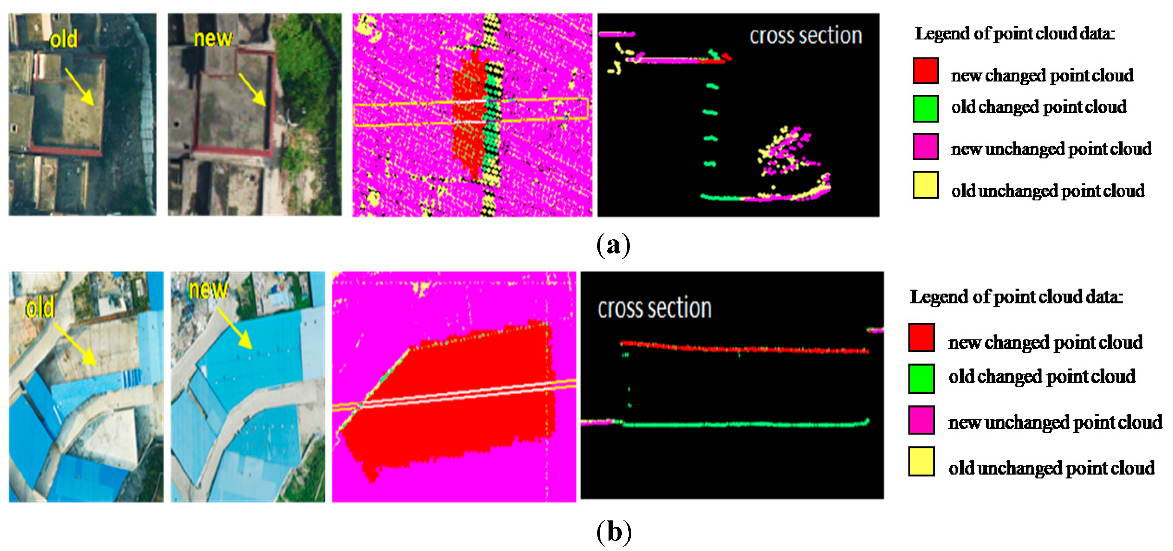
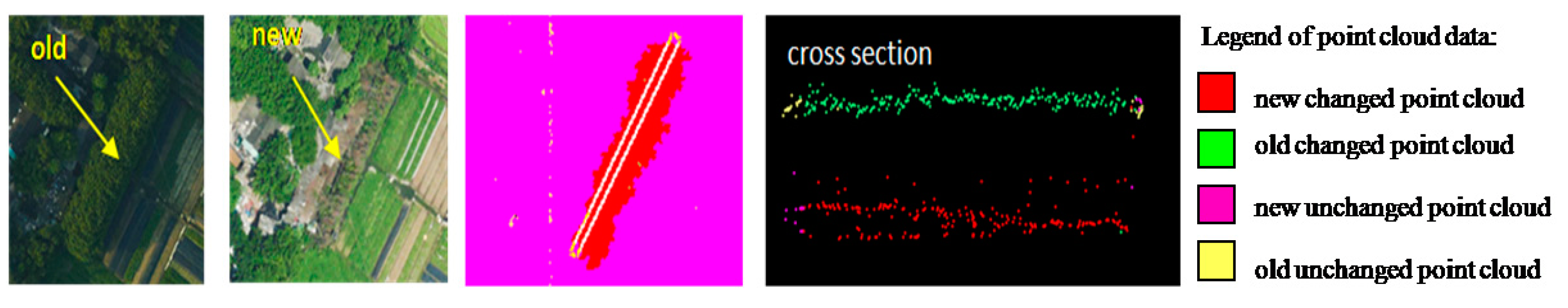
3.4. Discussion

Considering that only one area with a dataset is available for our experiment, two additional typical example scenarios, which are represented by two virtual models, are used for the analysis to further validate the effectiveness of our method. The illustrations of the two virtual models are shown as follows:

Case 1: Constructions built in urban areas that are not flat.

Figure 11. Cross-sections of old and new DSMs, where the black solid line BCDE represents the cross-section of the old DSM and the red and purple lines BHGFI represent the cross-section of the new DSM. The purple line BHGF represents the cross-section of a newly built building. The red line BCFI represents the cross-section of the new terrain.

Figure 11. Cross-sections of old and new DSMs, where the black solid line BCDE represents the cross-section of the old DSM and the red and purple lines BHGFI represent the cross-section of the new DSM. The purple line BHGF represents the cross-section of a newly built building. The red line BCFI represents the cross-section of the new terrain.

Figure 12. Cross-section of dDSM obtained by using the proposed method, where the black dash line is the zero height difference. The green solid line represents the threshold of height difference (T_hd), below which the dDSM value is set to zero. Thereafter, Obj1, Obj2, and Obj3 are obtained using the smoothness computation and connected component analysis technique.

Figure 12. Cross-section of dDSM obtained by using the proposed method, where the black dash line is the zero height difference. The green solid line represents the threshold of height difference (T_hd), below which the dDSM value is set to zero. Thereafter, Obj1, Obj2, and Obj3 are obtained using the smoothness computation and connected component analysis technique.

After obtaining the objects (e.g., Obj1, Obj2, and Obj3), their areas can be easily obtained. If the areas of the objects (e.g., Obj1, Obj2, and Obj3) are larger than the defined threshold (25 m² in this study), the height of the nDSM and the planarity ratio of the objects in the original point cloud data(e.g., Obj1, Obj2, and Obj3)will be calculated to evaluate whether the objects are buildings. Otherwise, the object will be discarded and considered unchanged. From Figure 11 and Figure 12, we observe that Obj1 and Obj2 are part of the newly built building. If the areas of Obj1 and Obj2 are larger than the defined threshold, two newly built buildings will be easily detected by using the proposed method. The changed object was considered two newly built buildings. However, the aim of this research is to locate the changed buildings and identify their change type. The accurate boundary of changed buildings should be further investigated. Obj3 represents the changed terrain. The height of Obj3 in the old and new nDSMs is zero. Thus, Obj3 can be easily excluded from the changed building.

Case 2: Constructions built on a hillside with a large inclination.

Figure 13. Cross-section of old and new DSMs, where the black solid line AB represents the cross-section of the old DSM, and the red and purple lines ACFGDEB represent the cross-section of the new DSM. The purple line CFGD represents the cross-section of the building. The red line ACDEB represents the cross-section of the new terrain.

Figure 13. Cross-section of old and new DSMs, where the black solid line AB represents the cross-section of the old DSM, and the red and purple lines ACFGDEB represent the cross-section of the new DSM. The purple line CFGD represents the cross-section of the building. The red line ACDEB represents the cross-section of the new terrain.

Figure 14. Cross-section of the dDSM obtained by using the proposed method, where the black dash line is the zero height difference. The two green solid lines represent the threshold of height difference. The height difference between the two green lines is set to zero (the absolute value of dDSM smaller than T_hd is set to zero). Thereafter, Obj1, Obj2, and Obj3 are obtained by using the smoothness computation and connected component analysis technique.

Figure 14. Cross-section of the dDSM obtained by using the proposed method, where the black dash line is the zero height difference. The two green solid lines represent the threshold of height difference. The height difference between the two green lines is set to zero (the absolute value of dDSM smaller than T_hd is set to zero). Thereafter, Obj1, Obj2, and Obj3 are obtained by using the smoothness computation and connected component analysis technique.

If the area of Obj2 is larger than the defined threshold (25 m² in this study), we can easily detect a newly built building by using the proposed method. Obj1 and Obj3 are the changed terrains. The height of Obj1 and Obj3 in the old and new nDSMs is zero. Thus, Obj1 and Obj3 can be easily excluded from the changed buildings.

The proposed method for building change detection obtains satisfactory results for most circumstances. Thus, the proposed method can be considered an effective method for building change detection with airborne LiDAR data. Furthermore, the automatic quality assessment of the result of building change detection guides the user to the most difficult case that the method might have difficulty. The proposed method is useful for practical projects and is also an important first attempt. The results show that, with the confidence index, users only need to check 140 objects of 342 changes.

However, our method still has problems that need to be resolved. First, the smoothness assumption in the dDSM meets most circumstances and shows good performance in our experiment. However, some buildings are small and irregularly shaped and have discontinuous roofs. Thus, we expect that the precision of the proposed change detection method will be worse. Further research on specific feature extraction methods of detecting such roof structures should be conducted. Second, the proposed method cannot determine the accurate boundary of the building because of the irregular distribution of points. We will attempt to combine the image information to extract the accurate boundary. Third, the automatic quality assessment expressed by the confidence index guides the user to the most likely wrong detections. The user only needs to check a part of the objects. However, for a confidence index lower than a certain value (0.8 in this test site), the relationship of the confidence index and wrong detections is unclear. In future research, we will attempt to use more datasets to further identify these relationships by using more effective features for the computation of the confidence index.

4. Conclusions

This study proposes a novel method of object-based analysis for building change detection from LiDAR point cloud data. The method can be applied to dense urban areas and forested areas, where buildings are composed of one or two prominent and smooth planes. The proposed method is relatively insensitive to vegetation and independent of terrain. A test data set covering approximately 8.5 km² with various types of buildings is used to validate the method. The results show that the proposed method can effectively locate the changed buildings and correctly determine their change type. The completeness and correctness of change detection for buildings larger than 50 m² are 97.8% and 91.2%, respectively. Furthermore, the confidence index of each changed object is computed to further decrease the manual workload. By using the confidence index, inspection can be guided to the most likely wrongly detected objects. Therefore, the method discussed in this study can effectively detect building changes. Thus, the manual workload is significantly reduced.

The major contributions of the proposed method are as follows: First, smoothness computation and RANSAC fitting are combined to determine the location of the changed objects. The object, which is the foundation of object-based analysis, is obtained by using the smoothness computation and connected component analysis technique. Thereafter, RANSAC fitting is applied to the candidates of the changed buildings to exclude trees from the changed buildings. Second, a self-diagnostic method for automatic quality assessment, which is an important first attempt, is proposed to reduce the post-processing time.

References

- Brunner, D.; Lemoine, G.; Bruzzone, L. Earthquake damage assessment of buildings using VHR optical and SAR imagery. IEEE Trans. Geosci. Remote Sens. 2010, 48, 2403–2420. [Google Scholar] [CrossRef]
- Bovolo, F.; Marin, C.; Bruzzone, L. A novel approach to building change detection in very high resolution SAR images. Proc. SPIE 2012, 8537. [Google Scholar] [CrossRef]
- Vu, T.T.; Ban, Y. Context-based mapping of damaged buildings from high-resolution optical satellite images. Int. J. Remote Sens. 2010, 31, 3411–3425. [Google Scholar] [CrossRef]
- Meng, Y.; Zhao, Z.; Du, X.; Peng, S. Building change detection based on similarity calibration. In Proceedings of the IEEE Fifth International Conference on Fuzzy Systems and Knowledge Discovery, Jinan, China, 18–20 October 2008; 2008. FSKD ’08. pp. 527–531. [Google Scholar]
- Argialas, D.P.; Michailidou, S.; Tzotsos, A. Change detection of buildings in suburban areas from high resolution satellite data developed through object based image analysis. Surv. Rev. 2013, 45, 441–450. [Google Scholar] [CrossRef]
- Li, P.; Xu, H.; Guo, J. Urban building damage detection from very high resolution imagery using OCSVM and spatial features. Int. J. Remote Sens. 2010, 31, 3393–3409. [Google Scholar] [CrossRef]
- Tang, Y.; Huang, X.; Zhang, L. Fault-tolerant building change detection from urban high-resolution remote sensing imagery. IEEE Geosci. Remote Sens. Lett. 2013, 10, 1060–1064. [Google Scholar] [CrossRef]
- Huang, X.; Zhang, L.; Zhu, T. Building change detection from multitemporal high-resolution remotely sensed images based on a morphological building index. IEEE J. Sel. Top. Appl. Earth Obs. Remote Sens. 2014, 7, 105–115. [Google Scholar] [CrossRef]
- Murakami, H.; Nakagawa, K.; Hasegawa, H. Change detection of buildings using an airborne laser scanner. ISPRS J. Photogramm. Remote Sens. 1999, 54, 148–152. [Google Scholar] [CrossRef]
- Vu, T.T.; Matsuoka, M.; Yamazaki, F. LIDAR-based change detection of buildings in dense urban areas. In Proceedings of 2004 IEEE International Geoscience and Remote Sensing Symposium, IGARSS ’04. Anchorage, AK, USA, 20–24 September 2004; Volume 5, pp. 3413–3416.
- Jung, F. Detecting building changes from multitemporal aerial stereo pairs. ISPRS J. Photogramm. Remote Sens. 2004, 58, 187–201. [Google Scholar] [CrossRef]
- Teo, T.; Shih, T. Lidar-based change detection and change type determination in urban areas. Int. J. Remote Sens. 2013, 34, 968–981. [Google Scholar] [CrossRef]
- Rottensteiner, F. Automated updating of building data bases from digital surface models and multi-spectral images: Potential and limitations. Int. Arch. Photogramm. Remote Sens. Spat. Inf. Sci. 2008, XXXVII, 265–270. [Google Scholar]
- Hermosilla, T.; Ruiz, L.A.; Recio, J.A.; Estornell, J. Evaluation of automatic building detection approaches combining high resolution images and LiDAR data. Remote Sens. 2011, 3, 1188–1210. [Google Scholar] [CrossRef]
- Grigillo, D.; Kosmatin Fras, M.; Petrovič, D. Automatic extraction and building change detection from digital surface model and multispectral orthophoto. Geod. Vestn. 2011, 55, 11–27. [Google Scholar] [CrossRef]
- Malpica, J.A.; Alonso, M.C.; Papí, F.; Arozarena, A.; Martínez De Agirre, A. Change detection of buildings from satellite imagery and lidar data. Int. J. Remote Sens. 2013, 34, 1652–1675. [Google Scholar] [CrossRef]
- Tian, J.; Cui, S.; Reinartz, P. Building change detection based on satellite stereo imagery and digital surface models. IEEE Trans. Geosci. Remote Sens. 2014, 52, 406–417. [Google Scholar] [CrossRef]
- Knudsen, T.; Olsen, B.P. Automated change detection for updates of digital map databases. Photogramm. Eng. Remote Sens. 2003, 69, 1289–1296. [Google Scholar] [CrossRef]
- Bouziani, M.; Goïta, K.; He, D. Automatic change detection of buildings in urban environment from very high spatial resolution images using existing geodatabase and prior knowledge. ISPRS J. Photogramm. Remote Sens. 2010, 65, 143–153. [Google Scholar] [CrossRef]
- Liu, Z.; Gong, P.; Shi, P.; Chen, H.; Zhu, L.; Sasagawa, T. Automated building change detection using UltraCamD images and existing CAD data. Int. J. Remote Sens. 2010, 31, 1505–1517. [Google Scholar] [CrossRef]
- Matikainen, L.; Hyyppä, J.; Ahokas, E.; Markelin, L.; Kaartinen, H. Automatic detection of buildings and changes in buildings for updating of maps. Remote Sens. 2010, 2, 1217–1248. [Google Scholar] [CrossRef]
- Silván-Cárdenas, J.L.; Wang, L. A multi-resolution approach for filtering LiDAR altimetry data. ISPRS J. Photogramm. Remote Sens. 2006, 61, 11–22. [Google Scholar] [CrossRef]
- Meng, X.; Wang, L.; Silván-Cárdenas, J.L.; Currit, N. A multi-directional ground filtering algorithm for airborne LIDAR. ISPRS J. Photogramm. Remote Sens. 2009, 64, 117–124. [Google Scholar] [CrossRef]
- Meng, X.; Wang, L.; Currit, N. Morphology-based building detection from airborne LIDAR data. Photogramm. Eng. Remote Sens. 2009, 75, 427–442. [Google Scholar]
- Zhang, J.; Lin, X.; Ning, X. SVM-based classification of segmented airborne LiDAR point clouds in urban areas. Remote Sens. 2013, 5, 3749–3775. [Google Scholar] [CrossRef]
- Axelsson, P. DEM generation from laser scanner data using adaptive TIN models. Int. Arch. Photogramm. Remote Sens. 2000, 33, 111–118. [Google Scholar]
- Kang, X.; Liu, J.; Lin, X. Streaming progressive TIN densification filter for airborne LiDAR point clouds using multi-core architectures. Remote Sens. 2014, 6, 7212–7232. [Google Scholar] [CrossRef]
- Zhu, X.; Toutin, T. Land cover classification using airborne LiDAR products in beauport, Québec, Canada. Int. J. Image Data Fusion 2013, 4, 252–271. [Google Scholar] [CrossRef]
- Fischler, M.A.; Bolles, R. Random sample consensus: A paradigm for model fitting with applications to image analysis and automated cartography. Commun. ACM 1981, 24, 381–395. [Google Scholar] [CrossRef]
- Besl, P.J.; McKay, N.D. A method for registration of 3D shapes. IEEE Trans. Pattern Anal. Mach. Intell. 1992, 14, 239–256. [Google Scholar] [CrossRef]
© 2014 by the authors; licensee MDPI, Basel, Switzerland. This article is an open access article distributed under the terms and conditions of the Creative Commons Attribution license (http://creativecommons.org/licenses/by/4.0/).
Share and Cite
Pang, S.; Hu, X.; Wang, Z.; Lu, Y. Object-Based Analysis of Airborne LiDAR Data for Building Change Detection. Remote Sens. 2014, 6, 10733-10749. https://doi.org/10.3390/rs61110733
Pang S, Hu X, Wang Z, Lu Y. Object-Based Analysis of Airborne LiDAR Data for Building Change Detection. Remote Sensing. 2014; 6(11):10733-10749. https://doi.org/10.3390/rs61110733
Chicago/Turabian StylePang, Shiyan, Xiangyun Hu, Zizheng Wang, and Yihui Lu. 2014. "Object-Based Analysis of Airborne LiDAR Data for Building Change Detection" Remote Sensing 6, no. 11: 10733-10749. https://doi.org/10.3390/rs61110733