Abstract
We present a novel technique to infer ground slope angle from waveform LiDAR, known as the independent slope method (ISM). The technique is applied to large footprint waveforms (∼60 m mean diameter) from the Ice, Cloud and Land Elevation Satellite (ICESat) Geoscience Laser Altimeter System (GLAS) to produce a slope dataset of near-global coverage at 0.5° × 0.5° resolution. ISM slope estimates are compared against high resolution airborne LiDAR slope measurements for nine sites across three continents. ISM slope estimates compare better with the aircraft data (R2 = 0.87 and RMSE = 5.16°) than the Shuttle Radar Topography Mission Digital Elevation Model (SRTM DEM) inferred slopes (R2 = 0.71 and RMSE = 8.69°). ISM slope estimates are concurrent with GLAS waveforms and can be used to correct biophysical parameters, such as tree height and biomass. They can also be fused with other DEMs, such as SRTM, to improve slope estimates.1. Introduction
Imaging the Earth’s surface using satellite Light Detection and Ranging (LiDAR) has shown great potential for mapping surface topography [1–3] and the distribution of vegetation parameters, e.g., forest height, from regional to global scales [4–10]. In particular, waveform LiDAR has proven its potential on a global scale via the Ice, Cloud and Land Elevation Satellite (ICESat) Geoscience Laser Altimeter System (GLAS). ICESat/GLAS was operational from 2003–2009 for about one month at a time, 1–3 times per year [11]. To date, this is the only mission to have recorded near global waveform LiDAR measurements of the Earth’s surface, providing data for studies of the oceans, cryosphere, atmosphere and biosphere.
A number of vegetation parameters, such as vegetation height, cover fraction, timber volume and biomass, can be estimated from GLAS waveforms [6,9,10,12–14]. However, accurate estimation of these parameters is compromised by the presence of sloped terrain. The LiDAR waveform reflected from a slope mixes with that of the overlying vegetation [1,15–17]. This dictates sloped terrain be a major factor affecting waveform signal-to-noise ratios [9] and, hence, induces difficulties in identifying ground returns. The failure to distinguish between signals from terrain and from vegetation can lead to waveform misinterpretations and inaccurate vegetation parameter retrieval [17]. Moreover, the waveform simulations of Rosette et al. [17] suggest that vegetation height retrievals for slopes ≥ 15° and high density canopy cover conditions (≥98%) are severely underestimated. In addition, footprint dimensionality can induce a directional bias and associated inconsistencies in waveform retrieved vegetation and terrain parameters; the dimensions of the elliptical GLAS footprints vary as a function of data acquisition period [18]. For instance, the first acquisition of Laser 1 is highly elliptical, and measurements are subject to an element of directionality, whereas the majority of Laser 3 acquisitions are more circular and will exhibit less directionality [18]. Accurate quantification of LiDAR inferred vegetation parameters is paramount in understanding the carbon cycle and forest ecosystem dynamics and in adequately assessing forest productivity and carbon sequestration rates [15,19]. Here, we develop a novel technique to retrieve slope estimates directly from LiDAR waveform returns, employing ICESat/GLAS waveforms for demonstration and validation purposes. The technique is expected to be applicable to all other waveform technologies, such as, for example, the Scanning LiDAR Imager of Canopies by Echo Recovery (SLICER) [20] and the Laser Vegetation Imaging Sensor (LVIS) [21].
In recent research, externally sourced slope information has been employed to filter suspected spurious waveform data from analysis [9,10,22]. For example, Simard et al. [9] and Los et al. [10] produced global forest height and global vegetation height distributions from GLAS data, employing the SRTM [23,24] data to derive close to spatially concurrent slope information to filter spurious data. However, as SRTM has a limited latitudinal extent between ±60°, reliable (direct inference) slope information is restricted between these boundaries. Extension beyond this latitudinal limit is possible by use of the Global 30 Arc-Second Elevation (GTOPO30) DEM product, which offers full global coverage between ±90°. However, the (global) vertical accuracy of this latter product (±18 m at 90% confidence) [25] is far less than that associated with SRTM equivalent measurements (±8m at 95% confidence) [23].
The uncertainties associated with the use of secondary DEM products depend on spatial resolution, location error and the amount of overlap. For example, the global SRTM data have a spatial resolution of 90 m (at the equator), and slope is estimated from two pixels on either side of a central pixel; this effectively reduces the resolution to 270 m, whereas the mean GLAS footprint size varies between 51 m and 102 m. This, combined with directional effects in the shuttle radar and location errors will introduce spatial discrepancies between GLAS footprints and corresponding SRTM DEM grid cells. By contrast, the method for retrieving ground slope in the present study utilises GLAS data, itself eradicating spatial inconsistencies, therefore minimising spatial uncertainties. Predicted within-footprint slopes should yield superior accuracy with respect to slope obtained from other sources (noted above), mainly due to identical spatial agreement between data.
2. Data
2.1. Waveform Data
In this study, we use the ICESat/GLAS land data (GLA14) product, release 33 [26,27]. Whilst in operation (2003–2009), GLAS emitted a Gaussian shaped laser pulse in the 532 and 1064 nm wavebands, approximately 0.75–0.90 m in width (corresponding to a 5–6-ns duration) at the full width half maximum (FWHM). The returned waveform energy profile (in volts, V) is utilised as a proxy to inform of intercepted surfaces, such as vegetation and/or the ground. The returned waveform was measured for a duration equivalent range (i.e., two-way travel) window of 81.6 m (544 ns) for earlier campaigns or 150 m (1000 ns) for later campaigns at 0.15-m (0.5 ns) intervals; the capture duration is expressed relative to a reference range time from the spacecraft [18]. GLAS was the first spaceborne waveform LiDAR instrument designed to offer almost continuous, near global coverage between ±86° latitude [12]. However, technical difficulties dictated that data were collected intermittently for its operational lifetime. This consisted of typically 2–3 periods of approximately one month-long data acquisitions per year [28,29], known as laser campaigns. GLAS footprints are variable size ellipses, with average dimensions (minor and major axes) of 52 m × 95 m for campaigns L1–L2 C and 47 m × 61 m for other campaigns, equivalent to an average circular diameter of approximately 64 m [30]. The returned waveforms contain various peaks according to intercepted surfaces and are fitted with up to six Gaussians (Figure 1) as described by Duong et al. [31], the sum of which define the “model alternate fit” return pulse. Note, not all waveforms exhibit such distinct ground returns, as in Figure 1 [16,17,32], which can infer difficulties in identifying the ground from waveform return profiles.
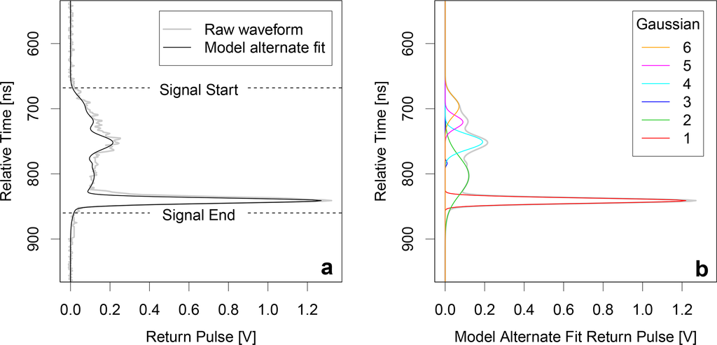
Table 1 provides GLA14 parameters used in this study in methodological processing (Section 3). Data without geographical coordinates or that exhibit cloud contamination (i_FRir_qaFlag ≠ 15) have been removed.

2.2. Validation Data
We tested ISM slope estimates on data from nine study sites where high resolution (≤1 mpixels) airborne LiDAR (ALS) (raster) data were available. These sites are located in Canada, Sweden, Germany, the Netherlands and Australia. Five sites are located within the northern boreal forests, three in temperate forests and one in a sub-alpine mountainous region.
The sites exhibit topographic variability, ranging from flat terrain to areas of ≥ 35° slope and cover major forest biomes. The ISM slope estimates were tested predominantly within forested regions (chosen to test the capability of retrieving slope estimates in the presence of vegetation). Test regions encompassed a diverse range of conditions, both in terms of terrain and vegetation cover, including conditions known to be problematic for the large footprint data of GLAS, e.g., sparse and dense canopy.
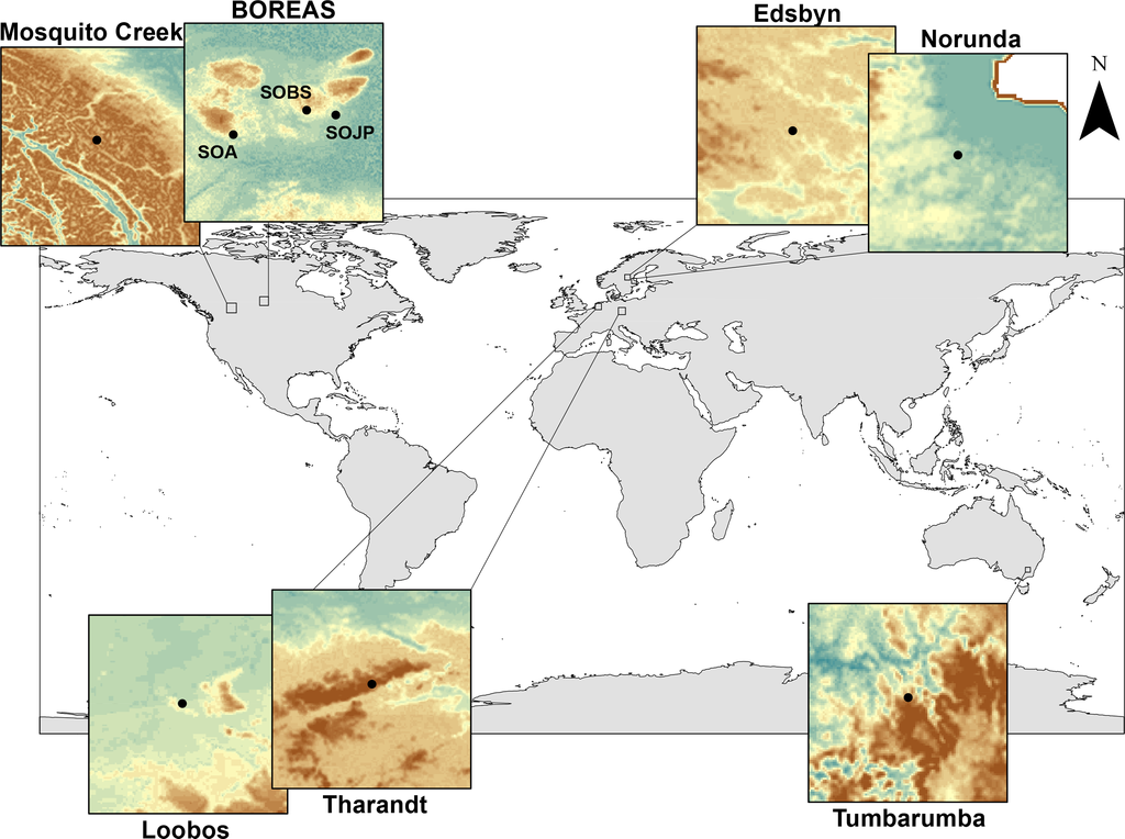
Three of the four Canadian sites are of the former southern BOREAS (Boreal Ecosystem–Atmosphere Study) study sites in Saskatchewan (CA); these exhibit a flat topography with relatively homogeneous (land-cover types) forested areas of Trembling aspen (SOA), black spruce (SOBS) and jack pine (SOJP) stands [33,34]. Airborne LiDAR data were collected and processed by the authors in August, 2008. Data at Mosquito Creek (MC), near Banff (CA), a mountainous region with a mean elevation of 2500 m a.s.l, were collected and processed by the authors in August 2011. Site topography is relatively complex with localised karst surface features, where forest coverage (20%) is generally restricted to valleys below 2100 m [35]. The European boreal site of Norunda (NR), near Uppsala, Sweden (S), exhibits a relatively homogeneous forest with flat topography and a high boulder presence, inducing greater terrain roughness [36,37]. Airborne LiDAR data were collected and processed by the authors in June 2011. The second Swedish boreal site near Edsbyn (ED) exhibits a relatively homogeneous forest with moderate topography and scattered wetlands throughout; here, airborne LiDAR data were processed and provided by Lantm¨ateriet (the Swedish land survey) as part of the Swedish national LiDAR dataset. At Loobos (LB), near Apeldoorn, the Netherlands (NL), the topography is generally flat with some local undulation and open areas throughout the forest [38]. At Tharandt (T), near Dresden, Germany (D), a relatively dense, multi-layered heterogeneous forest stand is situated on undulating terrain [39]. Data from these two sites were collected and processed by the authors in June 2010. The Australian (AUS) site is located near the Tumbarumba (TM) research station within the Bago State Forest, New South Wales, exhibiting a quite open canopy with relatively complex terrain [40]. Airborne LiDAR data were collected and processed by the authors during November 2009. Airborne LiDAR survey information is summarised in Table 2 and study site characteristics in Table 3. Study site geographic locations and terrain information are illustrated in Figure 2.
The interpolated SRTM DEM version 4.1, distributed by the Consultative Group for International Agriculture Research-Consortium for Spatial Information (CGIAR-CSI) [23,24], is employed to infer slope estimates at seven of the nine airborne LiDAR sites for comparison purposes. SRTM data are not available for > 60°N latitude, and therefore, the Edsbyn and Norunda sites (Sweden) are excluded from this comparison. Data from these two sites are useful as a demonstration of the proof of concept.
3. Method
3.1. Independent Slope Model (ISM)
Below, we derive the independent slope model (referred to as ISM throughout) and test it on GLAS waveforms. We use the GLAS model alternate fit return waveform, derived from the GLA14 Gaussian parameters (i_gpCntRngOff; see Figure 1), to infer slope. Estimating slope requires the accurate identification of the waveform ground return. In the case of GLAS, this is defined as the least elevated peak (greatest range) in the waveform profile between the i_SigBegOff (signal start) and i_SigEndOff (signal end) GLA14 elevation parameters (defined as the waveform extent; Figure 3a). We only analyse waveforms whose ground return maximum amplitude exceeds an imposed threshold of ≥ 0.2V. This threshold provided the best distinction (empirically) between returns representing ground only and mixed signal returns from ground and vegetation. A single Gaussian (Gf; Figure 3a) is fitted to the isolated waveform ground return, ensuring a single Gaussian representation, implemented to provide consistency in ground return shape. Ground return shape can be skewed, particularly when it represents mixed signal returns (as described above) and/or consists of multiple Gaussian fits.
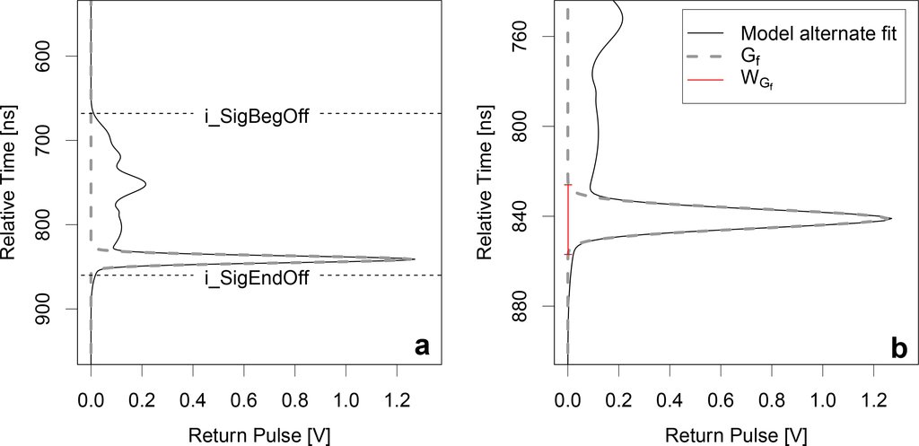
It is assumed that at an intensity threshold of 0.001 V, the width of Gf (Figure 3b) globally (for GLAS) represents the vertical displacement between the ground’s least and most elevated positions within the footprint. This intensity threshold was selected to exceed Gaussian distribution “tail” values, noted on average in the order of 10−9 here. The selected threshold is the maximum functional value before significant changes are noted in the recorded width of Gf. Lower thresholds yield no significant change in the width of Gf, but are more susceptible to being masked in Gaussian tail values, which can result in spurious measurements. The distance measure of Gf is used in combination with the mean footprint diameter to obtain slope (θ) by Equation (1).
3.1.1. Minimum Measurable Slope
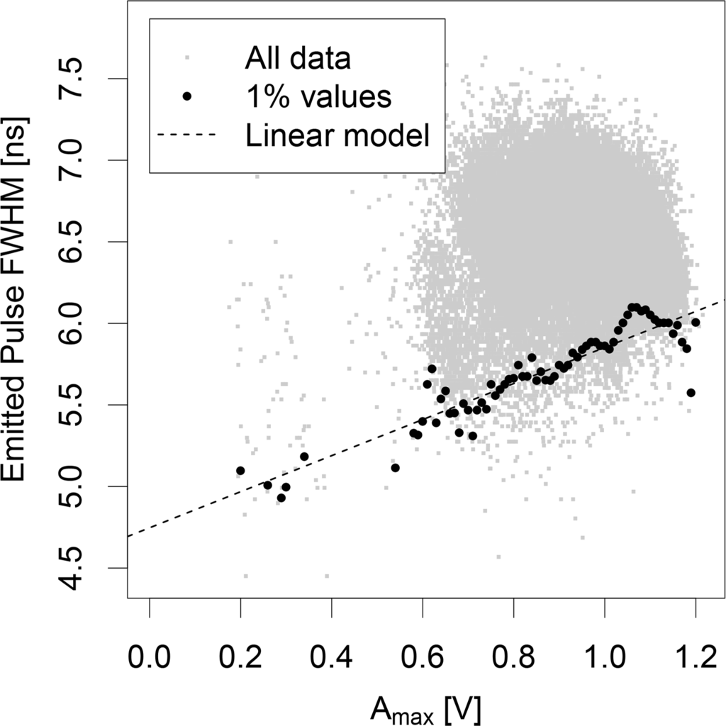
Returned waveforms will always exhibit a finite value of ▿E for (distinguishable) ground returns, because of the duration of the emitted signal and associated atmospheric attenuation. The implication is that even for completely flat surfaces, the lowest and highest within-footprint ground elevations differ, which translates to a finite slope measurement. An approach developed by Los et al. [10] for correcting vegetation height estimates can be applied here for similar purpose (with modification). The original method related vegetation height to the 5% values of the area under Gaussian 1. This yields a linear model that provides minimum measurable vegetation height estimates as a function of the area under Gaussian 1.
Based on this method, similar refinements can be applied in this study, where 1% FWHM values of Gf (in nanoseconds, ns) are linearly related to the returned waveform maximum amplitude (Amax), illustrated in Figure 4. This allows WGf (and subsequently, θ estimates from Equation (1) to be adjusted according to:
3.1.2. Gaussian Fit Filter
Quality control was performed on Gf, ensuring ground returns that are well represented by Gf are analysed for slope. To test this, the intensity profiles of the waveform ground return and Gf were isolated above an intensity threshold ≥ 0.001 V and compared. The implication being that these intensity profiles should be identical (i.e., R2 = 1.00) for perfect overlays of Gf and the waveform ground return, whereas poor fits are expected to yield reduced values of R2. Where resulting values of R2 ≤ 0.90, these waveforms are removed from further analysis, as results will unlikely represent true measurements.
3.2. Testing ISM Slope with ALS and SRTM
Both ISM and SRTM slope estimates were compared with slopes from high resolution ALS data for the 9 study sites. The comparison with SRTM data serves as a reference against which the performance of ISM is tested. ALS data were matched to unique GLAS footprints by overlaying the GLAS footprint perimeter (respecting size, azimuth rotation and location) over the ALS data and extracting data cells that were > 50% contained within the perimeter; slopes were calculated from the difference between minimum and maximum within-footprint elevations, divided by the mean footprint diameter (Equation (1)). SRTM slopes were calculated as the maximum difference between the centre SRTM cell located within the GLAS footprint and its eight neighbour cells [10].
4. Results and Discussion
4.1. Validation against Airborne LiDAR Slope
The comparisons of ISM retrieved slopes for all nine sites with airborne LiDAR (ALS) slopes are shown in Figure 5 and in Table 4. The equivalent comparisons for SRTM (and ISM) slopes with ALS for seven sites are shown in Figure 6 and Table 4. The results show a closer similarity between ISM slopes and ALS slopes (R2 = 0.87 and RMSE = 5.16°) compared to the SRTM slopes (R2 = 0.71 and RMSE = 8.69°). Additionally noted statistics in Table 4 are the: Kolmogorov-Smirnov statistic (D) [46], the fraction of (ISM/SRTM) predictions within a factor of two of the (ALS) observations (F2) and fractional bias (FB). Each corroborate that ISM slopes relate to ALS equivalents more closely than SRTM slopes.
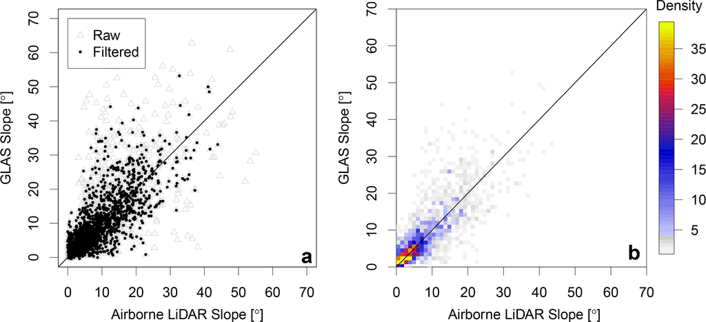
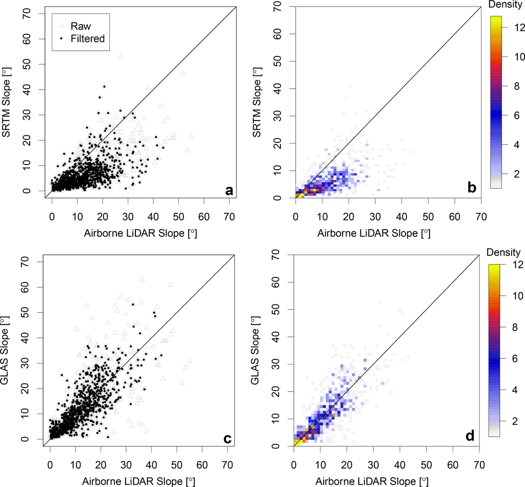
Figure 5a illustrates a comparison of ALS and ISM slopes for raw and filtered (according to Section 3.1.2) data; Figure 5b illustrates filtered data only, indicating the density of points per coloured pixel. Results suggest that the highest density of points occur near the 1:1 line (marked in both figures), up to an approximate maximum slope of 40°. Here, data filtering removed approximately 15% of all waveforms, and it is possible that some spurious data still remain in the current selection. Adjusting the acceptance threshold beyond R2 = 0.9 (see Section 3.1.2) will remove a larger proportion of spurious data, but this will be at the cost of removing too many reliable data.
Variability in results can arise from factors, such as ground roughness, terrain complexity and variations in the density of multi-layered canopies [1,16,47], all of which are unfavourable for the clear identification of waveform ground returns, particularly in large footprint systems.
4.2. Comparison with SRTM Slope
Figure 6a,b and Figure 6c,d illustrate the same as Figure 5a,b, but for ISM and SRTM and a corresponding subset of ISM and ALS data, respectively. It is highlighted that SRTM-derived slopes tend to underestimate ALS equivalents, an effect that becomes more prominent with increasing slope.
Figure 7a illustrates the absolute mean difference between observed (ALS) and predicted (ISM and SRTM) slope values as a function of 1° slope intervals, supporting that SRTM more severely underestimates slope than ISM equivalents with respect to ALS observations.
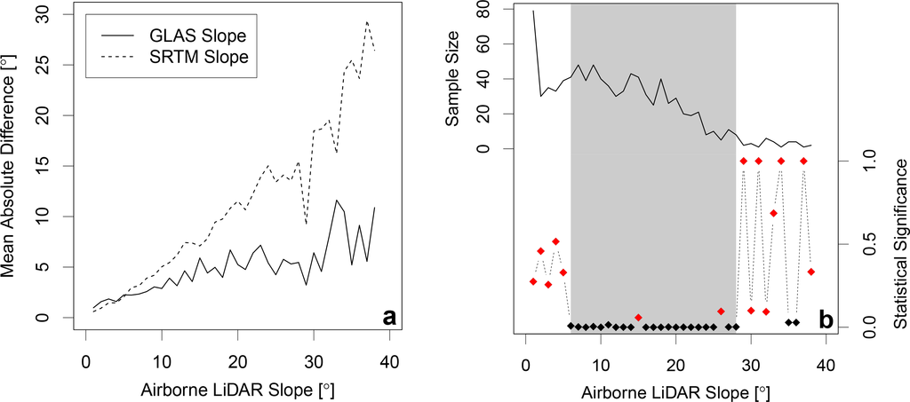
The statistical significance of the difference between ISM and SRTM slope estimates (at 1° intervals) was quantified with a non-parametric Mann–Whitney–Wilcoxon test [48]. Statistically significant differences are highlighted in Figure 7b as black points within the grey region, illustrated with respect to sample population. In particular, SRTM slopes are not statistically different from ALS equivalents up to 5° (Figure 7a), as well as for larger slopes (>28°); in the latter case, likely due to the small sample population (see Figure 7b). From 5°–28°, the majority of results exhibit statistically significant differences, as supported by Figure 7b. For slopes up to ∼28°, ISM slopes compare well with ALS equivalents; for slopes larger than 5°, they compare better than SRTM estimates. However, beyond 28°, further data would be required to yield a valid test agreement, as the sample is small and the population poorly represented.
The mean differences between ALS and ISM slopes exhibit less variability than the mean differences between ALS and SRTM slopes; this is an artefact of the cell size used to compare data, i.e., the number of samples in the ALS tiles is larger, and the variability as measured by the standard deviation is smaller. The large cell size of SRTM data smooths or flattens surface features found on the natural landscape, hence causing slope underestimates, whereas the smaller GLAS footprints/cells are more sensitive to surface features.
4.3. Global ISM Coverage
In accordance with GLAS coverage, a near-global ISM product was realised on a 0.5° × 0.5° spatial grid (Figure 8). Note that Greenland and Antarctica are not part of the GLA14 land surface altimetry data product [18].
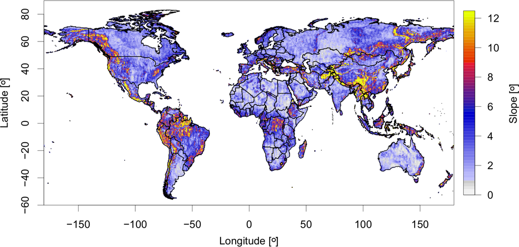
ISM slope from unique footprints are binned between 0°–70° at 0.5° intervals within each 0.5° × 0.5° grid cell, a method adopted from Los et al. [10]; values > 70° are deemed unrealistic and excluded. The value of each grid cell is the mean of all slopes between 0°–70° weighted by the frequency distribution of individual slopes (from the created histogram).
Visual inspection of the ISM product indicates most severe slopes occur in known mountainous regions, such as: the North American Rocky Mountains, the South American Andes and the Central Asian Himalayas. However, some indication is given to suggest that areas of the tropics exhibit significant slope, particularly within the Amazon basin and central Africa. Some features in tropical regions are real; however, ISM appears to often overestimate slope in these regions. This is suspected to be a legacy of dense, multi-layered vegetation canopies (cf. Section 4.4). Known areas with little terrain relief appear to be well represented by ISM inferred slope, particularly desert regions (e.g., the Sahara) and prairies (e.g., central Canada).
The ISM product exhibits a mean and standard deviation of 4.07° and 5.15°, respectively. It is estimated that approximately 73% of the observed land surface exhibits a slope ≤ 5°, where slopes from 5° to 25° cover approximately 27% of the land surface. Beyond 25°, slopes are observed to a maximum of 54°; however, these slopes constitute < 1% of the observed land surface. Even greater slopes are expected with finer spatial resolutions over mountainous regions. The coarse resolution of the current product is subject to high within-cell variability, the effect of which is diminished in taking the weighted mean of all slopes within a given grid cell. Whilst this is true for all cells, this effect is further exacerbated by the complex terrain that co-relates to mountainous regions, as a result a greater standard deviation, is noted for cells in such regions.
4.4. Benefits and Limitations of ISM
The ISM method for slope retrieval can be applied to any waveform LiDAR data source (not only GLAS, as employed here). The principles of the ISM essentially allow the retrieval of within-footprint vertical displacement. Provided the footprint’s mean diameter is known, slope can be retrieved from any footprint (dependent on waveform interpretation) from any waveform LiDAR data source with some minor changes required to accommodate instrument specific technicalities (e.g., emitted pulse length). If footprint dimensions are unavailable, they can be estimated using laser optical and physical (orientation) parameters [49]. Additionally, when used in conjunction with global GLAS data, the ISM is capable of providing slope estimates beyond the limits of other data sources. For example SRTM, used in most cases, offers limited coverage of ±60° latitude. The use of ISM with GLAS data allows slope retrievals to be made up to ±86° (limited by GLAS’ orbit). In addition, for dense canopies, SRTM penetrates to an inconsistent depth [50]. Hence, it neither represents a digital elevation model nor a digital surface model and cannot be assumed to be accurate for derivations of slope information.
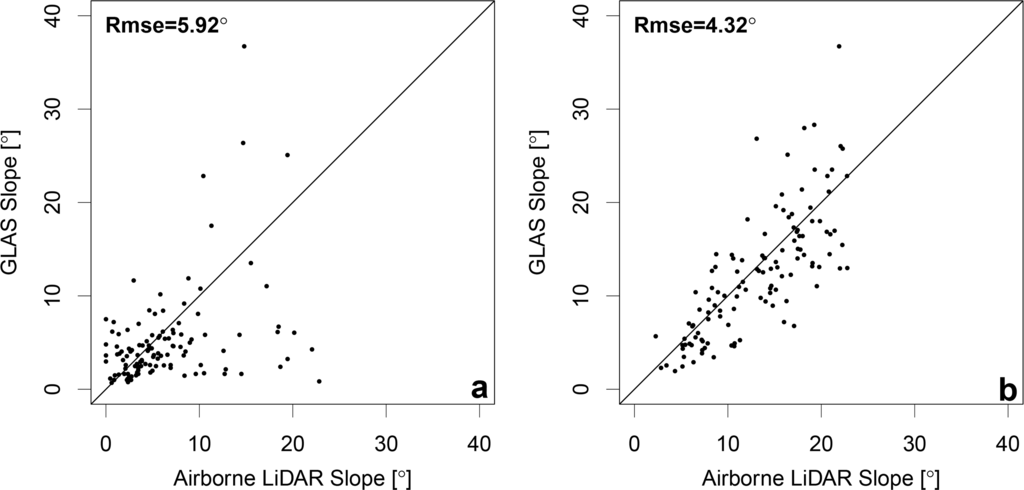
Based on ALS and ISM comparisons, the ISM product is capable of reducing slope uncertainties within GLAS footprints based on a simplistic, robust methodology. The results presented in this study are subject to large within-footprint terrain variability, which scales as a function of increasing footprint mean diameter. Hence, for waveform LiDAR systems yielding smaller footprints than those used in this study, it is not unreasonable to expect improved results with reduced uncertainty. This has been noted in SRTM data also [23,24]. ISM results are limited according to the quality of the returned waveform profile, which can be disturbed by high density and/or multi-layered vegetation canopies [22]. Such an effect has been noted to some extent in this study, particularly at the German site of Tharandt. Increased variability noted at this site (RMSE = 5.92°; Figure 9a) is a legacy of vegetation structure, not terrain complexity. This conclusion can be drawn as sites with low canopy density and high terrain complexity, for example Tumbarumba (Figure 9b), produced more coherent results (RMSE = 4.32°) within the same slope range (0° ≤ θ ≤ 25°). Here, in order to ensure that a like-for-like comparison was performed between sites without any sample bias, the same number of (filtered) data present at Tharandt were randomly sampled within the same ALS slope range from Tumbarumba.
5. Conclusions
This study has demonstrated the use of waveform LiDAR as a means of estimating ground slope with high accuracy when compared to high resolution airborne LiDAR equivalent results. Slope estimates were realised from Geoscience Laser Altimeter System (GLAS) waveforms via the implementation of the specifically developed Independent Slope Model (ISM), a novel technique for retrieving slope from waveform profiles. The current study has achieved the first quantitative retrieval of ground slope estimates from any waveform LiDAR instrument, offering improved accuracies on equivalent estimates from another spaceborne sensor and has potential to be applied to multiple instruments at a near global scale.
ISM slopes were compared with Shuttle Radar Topology Mission (SRTM)-derived slope information, as this has been employed in the published literature [9,10], such as to filter global ICESat/GLAS continuous waveform LiDAR data of spurious returns according to an imposed slope threshold. The current study has demonstrated that based on high resolution airborne LiDAR equivalent results, slope retrievals from SRTM data tend to underestimate surface slope across such footprints. The findings note that the ISM improves slope prediction results, with respect to equivalent SRTM results, when compared to airborne LiDAR-derived equivalents (R2 increases from 0.71 to 0.87, and RMSE decreases from 8.69° to 5.16°). Moreover, with the use of ISM in conjunction with global GLAS data, slope information can be retrieved from LiDAR waveforms outside the SRTM coverage region (±60°), up to ±86°, the latitudinal extent of GLAS coverage. The implications of such observations are that: (1) spatially concurrent slope information can be derived directly from all LiDAR waveform sources without the need of calibration and/or supplementary data; (2) accurate slope information can be derived beyond 60°, an SRTM coverage limitation; and (3) slope filtering can be applied to data with improved accuracy, as slope predictions from ISM appear more representative of the natural landscape than SRTM equivalent results.
Acknowledgments
ICESat/GLAS data were obtained from the National Snow and Ice Data Center (NSIDC), http://nsidc.org, and the interpolated SRTM-DEM version 4.1 data were obtained from the Consultative Group for International Agriculture Research-Consortium for Spatial Information (CGIAR-CSI), http://www.cgiar-csi.org. Airborne LiDAR data from the Canadian sites were obtained with support from the Natural Environment Research Council (NERC) (Grant NE/G000360/1) and the Canadian Consortium for LiDAR Environment Applications Research (C-CLEAR). Airborne LiDAR data for the European sites were acquired with support from NERC/the Applied Geomatics Research Group (AGRG)/FSF (Field Spectroscopy Facility) grant EU10-01 and NERC/GEF (Geophysical Equipment Facility) grants 909 and 933; for the Swedish site, Edsbyn, this was provided by Lantm¨ateriet (the Swedish land survey), Contract i2012/927. Airborne LiDAR data from Australia were collected with support from (National Centre for Earth Observation) NCEO EO mission support 2009 (NE/R8H1282). Special thanks to the Applied Geomatics Research Group (AGRG) in Nova Scotia, the NERC Airborne Research and Survey Facility (ARSF) and Airborne Research Australia (ARA) for carrying out the airborne campaigns. The authors acknowledge support from Lund University and from LUCCI (Lund University Centre for Studies of Carbon Cycle and Climate Interactions), Linnaeus center funded by the Swedish Research Council, Vetenskapsrådet.
Author Contributions
C. Mahoney derived the method for slope derivation, N. Kljun coordinated the airborne LiDAR surveys at SOA, SOBS, SOJP together with C. Hopkinson and L. Chasmer, at Tumbarumba together with E. van Gorsel and J.M. Hacker, and at Norunda, Loobos, and Tharandt; C. Hopkinson coordinated the airborne LiDAR survey at Mosquito Creek together with L. Chasmer; C. Mahoney and L. Chasmer preprocessed the airborne LiDAR data; C. Mahoney processed the ICESat/GLAS data; C. Mahoney wrote the paper with support from N. Kljun and S. Los.
Conflicts of Interest
The authors declare no conflicts of interest.
References
- Chen, Q. Assessment of terrain elevation derived from satellite laser altimetry over mountainous forest areas using airborne lidar data. ISPRS J. Photogramm. Remote Sens 2010, 65, 111–122. [Google Scholar]
- Rosette, J.A.B.; North, P.R.J.; Suárez, J.C.; Los, S.O. Uncertainty within satellite LiDAR estimations of vegetation and topography. Int. J. Remote Sens 2010, 31, 1325–1342. [Google Scholar]
- Jia, Y.; Zhang, X.; Lv, Y.; Lang, X. Lidar echo characteristics analysis for stepped terrain. Proc. SPIE 2013, 8759. [Google Scholar] [CrossRef]
- Drake, J.B.; Knox, R.G.; Dubayah, R.O.; Clark, D.B.; Condit, R.; Blair, J.B.; Hofton, M. Above-ground biomass estimation in closed canopy neotropical forests using lidar remote sensing: Factors affecting the generality of relationships. Glob. Ecol. Biogeogr 2003, 12, 147–159. [Google Scholar]
- Hese, S.; Lucht, W.; Schmullius, C.; Barnsley, M.; Dubayah, R.; Knorr, D.; Neumann, K.; Riedel, T.; Schroter, K. Global biomass mapping for an improved understanding of the CO2 balance-the Earth observation mission Carbon-3D. Remote Sens. Environ 2005, 94, 94–104. [Google Scholar]
- Nelson, R.; Ranson, K.J.; Sun, G.; Kimes, D.S.; Kharuk, V.; Montesano, P. Estimating Siberian timber volume using MODIS and ICESat/GLAS. Remote Sens. Environ 2009, 113, 691–701. [Google Scholar]
- Dubayah, R.O.; Sheldon, S.L.; Clark, D.B.; Hofton, M.A.; Blair, J.B.; Hurtt, G.C.; Chazdon, R.L. Estimation of tropical forest height and biomass dynamics using lidar remote sensing at La Selva, Costa Rica. J. Geophys. Res 2010, 115. [Google Scholar] [CrossRef]
- Lefsky, M.A. A global forest canopy height map from the Moderate Resolution Imaging Spectroradiometer and the Geoscience Laser Altimeter System. Geophys. Res. Lett 2010, 37. [Google Scholar] [CrossRef]
- Simard, M.; Pinto, N.; Fisher, J.B.; Baccini, A. Mapping forest canopy height globally with spaceborne lidar. J. Geophys. Res 2011, 116. [Google Scholar] [CrossRef]
- Los, S.O.; Rosette, J.A.B.; Kljun, N.; North, P.R.J.; Suárez, J.C.; Hopkinson, C.; Hill, R.A.; Chasmer, L.; van Gorsel, E.; Mahoney, C.; et al. Vegetation height products between 60°N and 60°S from ICESat GLAS data. Geosci. Model Dev 2012, 4, 2327–2363. [Google Scholar]
- Zwally, H.J.; Schutz, B.; Abdalati, W.; Abshire, J.; Bentley, C.; Brenner, A.; Bufton, J.; Dezio, J.; Hancock, D.; Harding, D.; et al. ICESat’s laser measurements of polar ice, atmosphere, ocean, and land. J. Geodyn 2002, 34, 405–445. [Google Scholar]
- Rosette, J.A.B.; North, P.R.J.; Suárez, J.C. Vegetation height estimates for a mixed temperate forest using satellite laser altimetry. Int. J. Remote Sens 2008, 29, 1475–1493. [Google Scholar]
- Lefsky, M.A.; Cohen, W.B.; Parker, G.G.; Harding, D.J. Lidar remote sensing for ecosystem studies. Bioscience 2002, 52, 19–30. [Google Scholar]
- Lefsky, M.A.; Harding, D.J.; Keller, M.; Cohen, W.B.; Carabajal, C.C.; Espirito-Santo, F.D.B.; Hunter, M.O.; de Oliveira, R. Estimates of forest canopy height and aboveground biomass using ICESat. Geophys. Res. Lett 2005, 32. [Google Scholar] [CrossRef]
- Sun, G.; Ranson, K.J.; Kimes, D.S.; Blair, J.B.; Kovacs, K. Forest vertical structure from GLAS: An evaluation using LVIS and SRTM data. Remote Sens. Environ 2008, 112, 107–117. [Google Scholar]
- North, P.R.J.; Rosette, J.A.B.; Suárez, J.C.; Los, S.O. A Monte Carlo radiative transfer model of satellite waveform LiDAR. Int. J. Remote Sens 2010, 31, 1343–1358. [Google Scholar]
- Rosette, J.A.B.; North, P.R.J.; Rubio-Gil, J.; Cook, B.; Los, S.; Suaŕez, J.; Sun, G.; Ranson, J.; Blair, J.B. Evaluating prospects for improved forest parameter retrieval from satellite LiDAR using a physically-based radiative transfer model. IEEE J. Sel. Topics Appl. Earth Observ 2013, 6, 45–53. [Google Scholar]
- NSIDC. ICESat/GLAS GLA14 Release 33 Data at NSIDC, 2012. National Snow and Ice Data Center. Available online: http://nsidc.org/data/icesat/index.html (accessed on 9 October 2012).
- Allouis, T.; Durrieu, S.; Véga, C.; Couteron, P. Stem volume and above-ground biomass estimation of individual pine trees from LiDAR data: Contribution of full-waveform signals. IEEE J. Sel. Topics Appl. Earth Observ 2012, 6, 924–934. [Google Scholar]
- Hofton, M.A.; Blair, J.B.; Minster, J.B.; Ridgway, J.R.; Williams, N.P.; Bufton, J.L.; Rabine, D.L. An airborne scanning laser altimetry survey of Long Valley, California. Int. J. Remote Sens 2000, 21, 2413–2437. [Google Scholar]
- Blair, J.B.; Rabine, D.L.; Hofton, M.A. The Laser Vegetation Imaging Sensor (LVIS): A medium-altitude, digitization-only, airborne laser altimeter for mapping vegetation and topography. ISPRS J. Photogramm. Remote Sens 1999, 54, 115–122. [Google Scholar]
- Pang, Y.; Lefsky, M.; Anderson, H.; Miller, M.E.; Sherrill, K. Validation of the ICESat vegetation product using crown-area-weighted mean height derived using crown delineation with discrete return lidar data. Can. J. Remote Sens 2008, 34, S471–S484. [Google Scholar]
- Rodriguez, E.; Morris, C.S.; Belz, J.E.; Chaplin, E.C.; Martin, J.M.; Daffer, W.; Hensley, S. An Assessment of the SRTM Topographic Products; Technical Report JPL D-31639; NASA Jet Propulsion Laboratory: Pasadena, CA, USA, 2005. [Google Scholar]
- Jarvis, A.; Reuter, H.I.; Nelson, A.; Guevara, A. Hole-Filled SRTM for the Globe Version 4, 2008. CGIAR-CSI SRTM 90 m Database. Available online: http://srtm.csi.cgiar.org (accessed on 25 July 2012).
- GTOPO30 Documentation; Technical Report; US Geological Survey Center for Earth Resources Observation and Science: Sioux Falls, SD, USA, 2012.
- Zwally, H.; Schutz, H.; Bentley, C.; Bufton, J.; Herring, T.; Minster, J.; Spinhirne, J.; Thomas, R. GLAS/ICESat L2 Global Land Surface Altimetry Data, V33; National Snow and Ice Data Center: Boulder, CO, USA, 2011. [Google Scholar]
- Brenner, A.C.; Zwally, H.J.; Bentley, C.R.; Csathó, B.M.; Harding, D.J.; Hofton, M.A.; Minster, J.B.; Roberts, L.; Saba, J.L.; Thomas, R.H.; et al. Geoscience Laser Altimeter System (GLAS): Derivation of Range and Range Distributions From Laser Pulse Waveform Analysis for Surface Elevations, Roughness, Slope, and Vegetation Heights; Algorithm Theoretical Basis Document 4.1; NASA Goddard Space Flight Center: Greenbelt, MD, USA, 2003. [Google Scholar]
- Harding, D.J.; Carabajal, C.C. ICESat waveform measurements of within-footprint topographic relief and vegetation vertical structure. Geophys. Res. Lett 2005, 32. [Google Scholar] [CrossRef]
- Schutz, B.E.; Zwally, H.J.; Shuman, C.A.; Hancock, D.; DiMarzio, J.P. Overview of the ICESat mission. Geophys. Res. Lett 2005, 32. [Google Scholar] [CrossRef]
- Abshire, J.B.; Sun, X.; Riris, H.; Sirota, J.M.; McGarry, J.F.; Palm, S.; Yi, D.; Liiva, P. Geoscience Laser Altimeter System (GLAS) on the ICESat mission: On-orbit measurement performance. Geophys. Res. Lett 2005, 32. [Google Scholar] [CrossRef]
- Duong, H.; Pfeifer, N.; Lindenbergh, R. Analysis of repeated ICESat full waveform data: Methodology and leaf-on/leaf-off comparison. Proceedings of Workshop on 3D Remote Sensing in Forestry, Vienna, Austria, 13–15 February 2006; pp. 239–248. Available online: http://www.rali.boku.ac.at/3drsforestry.html (accessed on 15 October 2014).
- Lefsky, M.A.; Keller, M.; Pang, Y.; De Camargo, P.B.; Hunter, M.O. Revised method for forest canopy height estimation from Geoscience Laser Altimeter System waveforms. J. Appl. Remote Sens 2007, 1. [Google Scholar] [CrossRef]
- Barr, A.G.; Morgenstern, K.; Black, T.A.; McCaughey, J.H.; Nesic, Z. Surface energy balance closure by eddy covariance method above three boreal forest stands and implications for the measurement of CO2 fluxes. Agr. Forest Meteorol 2006, 140, 322–337. [Google Scholar]
- Kljun, N.; Black, T.A.; Griffis, T.J.; Barr, A.G.; Gaumont-Guay, D.; Morgenstern, K.; McCaughey, J.H.; Nesic, Z. Response of net ecosystem productivity of three boreal forest stands to drought. Ecosystems 2006, 9, 1128–1144. [Google Scholar]
- Hopkinson, C. Investigating Spatio-Temporal Variability of Hydrological Components in the Canadian Rockies. PhD. Thesis. Wilfrid Laurier University, Waterloo, Canada, 2002. [Google Scholar]
- Lindroth, A.; Grelle, A.; Morén, A.S. Long-term measurements of boreal forest carbon balance reveal large temperature sensitivity. Glob. Change Biol 1998, 4, 443–450. [Google Scholar]
- Feigenwinter, C.; Mölder, M.; Lindroth, A.; Aubinet, M. Spatiotemporal evolution of CO2 concentration, temperature, and wind field during stable nights at the Norunda forest site. Agr. Forest Meteorol 2010, 150, 692–701. [Google Scholar]
- Dolman, A.J.; Moors, E.J.; Elbers, J.A. The carbon uptake of a mid latitude pine forest growing on sandy soil. Agr. Forest Meteorol 2002, 111, 157–170. [Google Scholar]
- Grünwald, T.; Bernhofer, C. A decade of carbon, water and energy flux measurements of an old spruce forest at the Anchor Station Tharandt. Tellus B 2007, 59, 387–396. [Google Scholar]
- Leuning, R.; Cleugh, H.A.; Zegelin, S.J.; Hughes, D. Carbon and water fluxes over a temperate Eucalyptus forest and a tropical wet/dry savanna in Australia: Measurements and comparison with MODIS remote sensing estimates. Agr. Forest Meteorol 2005, 129, 151–173. [Google Scholar]
- McCaughey, J.H.; Barr, A.G.; Black, T.A.; Nesic, Z.; Morgenstern, K.; Griffis, T.; Gaumont-Guay, D. Carbon and energy exchanges at three boreal forest sites in BERMS study region in 2000 and 2001. Proceedings of the 25th Conference on Agricultural and Forest Meteorology, Norfolk, VA, USA, 13–24 May 2002.
- Chen, J.M.; Govind, A.; Sonnentag, O.; Zhang, Y.; Barr, A.; Amiro, B. Leaf area index measurements at Fluxnet-Canada forest sites. Agr. Forest Meteorol 2006, 140, 257–268. [Google Scholar]
- Gaumont-Guay, D.; Black, T.A.; McCaughey, H.; Barr, A.G.; Krishnan, P.; Jassal, R.S.; Nesic, Z. Soil CO2 efflux in contrasting boreal deciduous and coniferous stands and its contribution to the ecosystem carbon balance. Glob. Change Biol 2009, 15, 1302–1319. [Google Scholar]
- Lagergren, F.; Eklundh, L.; Grelle, A.; Lundblad, M.; Mölder, M.; Lankreijer, H.; Lindroth, A. Net primary production and light use efficiency in a mixed coniferous forest in Sweden. Plant Cell Environ 2004, 28, 412–423. [Google Scholar]
- van Gorsel, E.; Leuning, R.; Cleugh, H.A.; Keith, H.; Kirschbaum, M.U.F.; Suni, T. Application of an alternative method to derive reliable estimates of nighttime respiration from eddy covariance measurements in moderately complex topography. Agr. Forest Meteorol 2008, 148, 1174–1180. [Google Scholar]
- Massey, F.J. The Kolmogorov-Smirnov test for goodness of fit. J. Am. Stat. Assoc 1951, 46, 68–78. [Google Scholar]
- Mahoney, C. Improved Estimates of Vegetation and Terrain Parameters from Waveform LiDAR. PhD. Thesis. Swansea University, Swansea, UK, 2013. [Google Scholar]
- Mann, H.B.; Whitney, D.R. On a test of whether one of two random variables is stochastically larger than the other. Ann. Math. Stat 1947, 18, 50–60. [Google Scholar]
- Svelto, O. Principles of Lasers, 5th ed.; Springer: Berlin, Germany, 2010. [Google Scholar]
- NASA. Shuttle Radar Topography Mission Frequently Asked Questions. NASA Jet Propulsion Laboratory, 2005. Available online: http://www2.jpl.nasa.gov/srtm/faq.html (accessed on 11 March 2014).
© 2014 by the authors; licensee MDPI, Basel, Switzerland This article is an open access article distributed under the terms and conditions of the Creative Commons Attribution license (http://creativecommons.org/licenses/by/4.0/).