Ultraviolet Fluorescence LiDAR (UFL) as a Measurement Tool for Water Quality Parameters in Turbid Lake Conditions

 ,
,  and
and 
Abstract
: Despite longstanding contributions to oceanography, similar use of fluorescence light detection and ranging (LiDAR) in lake settings is not routine. The potential for ship-mounted, multispectral Ultraviolet Fluorescence LiDAR (UFL) to provide rapid, high-resolution data in variably turbid and productive lake conditions are investigated here through a series of laboratory tank and field measurements carried out on Lake Balaton, Hungary. UFL data, calibrated empirically to a set of coinciding conventionally-analyzed samples, provide simultaneous estimates of three important parameters-chlorophyll a(chla), total suspended matter (TSM) and colored dissolved organic matter (CDOM). Successful UFL retrievals from both laboratory and field measurements were achieved for chla (0.01–378 mg·m−3; R = 0.83–0.92), TSM (0.1–130 g·m−3; R = 0.90–0.96) and CDOM (0.003–0.125 aCDOM(440); R = 0.80–0.97). Fluorescence emission at 685 nm is shown through tank measurements to display robust but distinct relationships with chla concentration for the two cultured algae species investigated (cyanobacteria, Cylindrospermopsis raciborskii, and chlorophyta, Scenedesmus armatus). The ratio between fluorescence emissions measured at 650 nm, related to the phycocyanin fluorescence maximum, to that at 685 nm is demonstrated to effectively distinguish these two species. Validation through both laboratory measurements and field measurements confirmed that site specific calibration is necessary. This study presents the first known assessment and application of ship-mounted fluorescence LiDAR in freshwater lake conditions and demonstrates the use of UFL in measuring important water quality parameters despite the more complicated hydro-optic conditions of inland waters.1. Introduction
Laser induced fluorescence light detection and ranging (LiDAR) systems have an extensive history of providing data for oceanographic research and monitoring [1,2]. Measurements in open ocean, coastal zone, estuarine and lagoon settings have been made using diverse airborne, ship-mounted and stationary platform-based instruments. These include fluorosensor, hyperspectral and imaging LiDAR instruments, using varying laser types, sensor geometries, and optimized for the retrieval of specific parameters [3,4]. Principle applications of fluorescence LiDAR systems in the marine environment have included the detection of oil spills and other pollutants [4–8], quantification and characterization of phytoplankton (through the pigment chlorophyll a (chla)) and colored dissolved organic matter (CDOM) [9,10], as well as the estimation of total suspended matter (TSM) concentrations in the sea surface layer [11]. Fluorescence LiDAR datasets have also successfully served as validation for satellite-derived oceanographic measurements [12–14].
Despite the inclusion of freshwater systems in some early trials and applications of airborne fluorescence LiDAR [15], its use in the research and monitoring of inland waters remains limited with only a few exceptions (e.g., [16,17]). As in marine settings, fluorescence spectroscopy has provided invaluable insight into a range of processes and phenomena in lakes, including the characterization of phytoplankton, pollutants and dissolved organic matter [18–23]. Combining the technologies of LiDAR and fluorescence spectroscopy allows the potential to detect fluorescence features of lake water in situ and non-intrusively, while adding a cohesive spatial component. Likewise, the spatial scale associated with ship-mounted measurements (1–5 m) may be well suited to the detection and interpretation of small to medium-scale ecological processes in lakes, and the provision of abundant validation data for satellite based measurements.
The potential of the Ultraviolet Fluorescence LiDAR (UFL) of the Shirshov Institute of Oceanology to simultaneously detect multiple water quality parameters of interest within the contexts of lake management and research—chla, TSM and CDOM—could be particularly advantageous in optically complex lake waters. Under such conditions this proves to be an important challenge for passive remote sensing techniques as a result of the overlapping and non-linearly related spectral reflectance and absorption features of the individual parameters [24–26]. UFL measures these parameters in distinct, non-overlapping channels, and with a strong signal as a result of the active, laser-induced fluorescence and backscattering. The possible impact of this same optical complexity on fluorescence LiDAR parameter retrieval, especially at the high parameter concentrations characteristic of many lakes relative to open ocean conditions remains to be investigated. At these higher concentrations, backscattering and absorbance of the emitted fluorescence may hinder the reliable interpretation of the fluorescence signal. Likewise the presence of multiple phytoplankton species with varying chla fluorescence efficiencies and accessory pigments may hinder our ability to derive a robust relationship between chla fluorescence emission intensity and phytoplankton biomass. On the other hand, fluorescence of accessory pigments specific to different phytoplankton divisions may provide the opportunity to differentiate these through their UFL fluorescence spectra. Cyanobacteria are of particular interest in this regard; whereas chlorophyta and diatom species typically dominate in Lake Balaton, for example, cyanobacteria blooms tend to be highly productive, have a toxic potential and are thus of concern from a monitoring perspective.
This study investigates whether UFL can provide reliable chlorophyll a, suspended sediment and CDOM measurements in lake environments that are much more optically complex than typical open ocean waters, where fluorescence LiDAR measurements have generally been carried out. The instrument was tested on a wide range of conditions encountered across Lake Balaton and through controlled laboratory tank experiments. The laboratory tank experiments generally extend the concentration ranges encountered in the field during the study period, and as such extend interpretation of the possible applicability to other lake sites and conditions. Retrieval performance of UFL is considered relative to coinciding samples analyzed according to the standard procedures of the Balaton Limnological Nutrient Cycling Laboratory.
2. Study Site
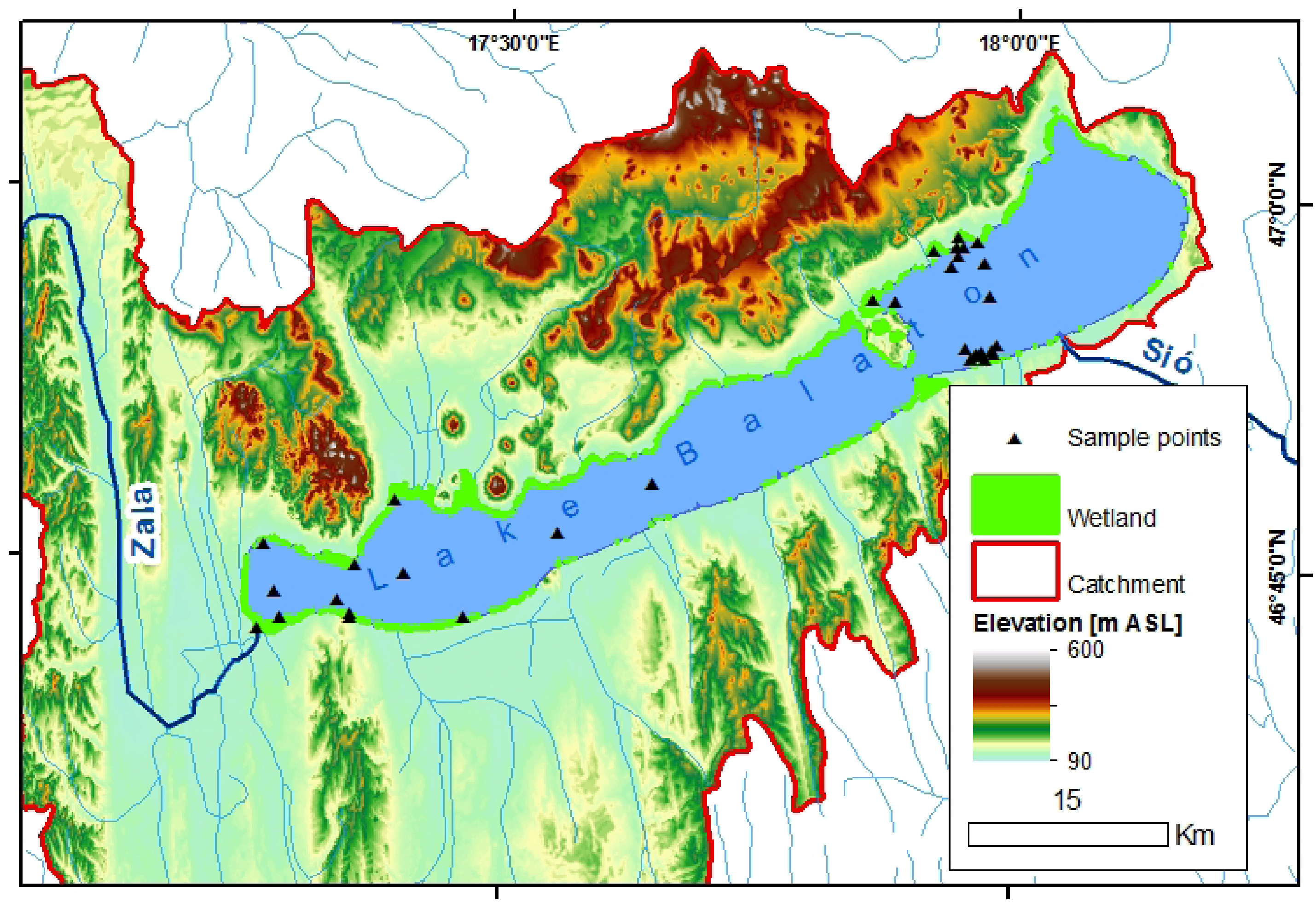
Field measurements were carried out on Lake Balaton (Figure 1) from 4 to 8 June 2012. Located in the Western Transdanubian region of Hungary, Lake Balaton is the largest shallow lake in Central Europe, with a surface area of 597 km2 and an average depth of only 3.3 m. Owing to its shallow depth and the easy resuspension of fine-grained bottom sediment, Lake Balaton is a vertically well-mixed and turbid system. Suspended matter is generally controlled by wind-induced resuspension of benthic sediment, influenced by spatially variable local topography surrounding the lake (Figure 1), sediment texture and bathymetry, as well as spatially and temporally variable wind conditions.
A longitudinal trophic gradient persists in Lake Balaton with generally higher phytoplankton biomass and associated chlorophyll a concentrations in the southwestern-most basin (generally considered eutrophic to hypertrophic), declining to the northeastern-most basin (generally considered mesotrophic) [27,28]. This is related to the only major inflow into the lake, the nutrient rich Zala River, in the southwestern-most basin (Figure 1) and the predominantly southwest to northeast circulation. The general southwest-northeast CDOM gradient has likewise been found to be controlled by inflow from the Zala River, and subsequent circulation and photodegradation from southwest to northeast [22].
3. Materials and Methods
3.1. Ultraviolet Fluorescence LiDAR (UFL)
The series of Ultraviolet Fluorescence LiDAR (UFL) instruments was developed by the Shirshov Institute of Oceanology of the Russian Academy of Sciences [11,29]. Version UFL-9, detailed in Table 1, was used in this study, and makes use of dual neodymium-doped yttrium aluminum garnet (Nd:YAG) excitation laser pulses (of wavelengths 355 (1.5 mJ energy) and 532 nm (3 mJ energy)) emitted at a frequency of 2 Hz for a duration of 6 ns each. In the current work, only the 355 nm excitation laser was used. Dimensions and weight of the UFL-9 are 100 × 70 × 30 cm and 35 kg, including water resistant housing. Power (220 V, 50 Hz, 120 W) can be supplied from an onboard network or a portable generator. Measurements can be taken from a distance of between 1.5 and 25 m above the water surface (through adjusting the length of the Kepler telescope accordingly), at an incidence angle of between 10° and 60°, and are thus well suited to ship-mounted measurement aboard a wide range of research vessels, including smaller boats often necessary in limnological research. The measurement frequency is dependent upon the speed of the transporting vehicle, and generally provides remotely sensed point measurements along track every 1–5 m. Low-pass filtering is used, with smoothing by moving averaging over a window of three points. The instrument is directly linked to a GPS and all collected data points are geo-tagged.
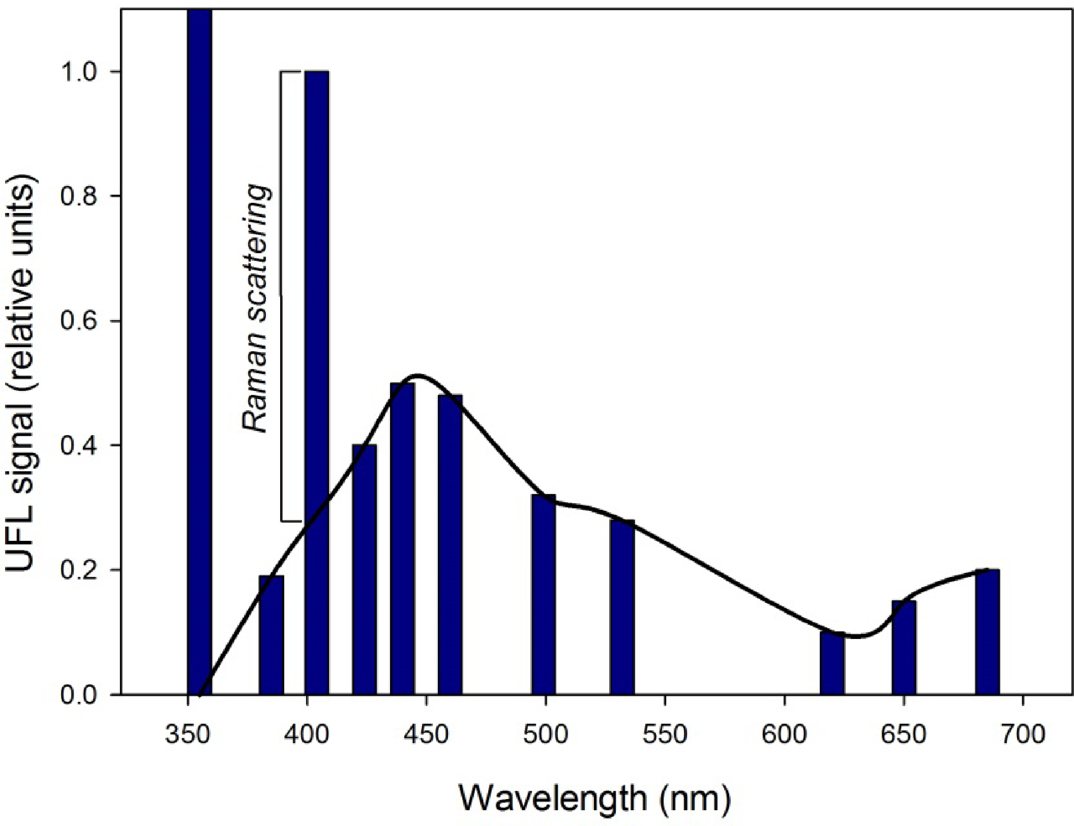
The backscattering and fluorescence emission spectra are detected across 11 receiver channels, centered at 355, 385, 404, 424, 440, 460, 499, 532, 620, 651 and 685 nm. Photomultipliers are used as receivers, and a four-channel beam splitter using interference filters is optimized to simultaneously detect water Raman scattering (at 404 nm from the 355 nm excitation laser pulse, at 651 nm from the 532 nm excitation laser pulse) and key water quality parameters, chla and CDOM through their fluorescence peaks (685 and 440 nm respectively), as well as TSM through backscattering of the 355 nm excitation laser pulse. Fluorescence emission maxima and backscattering associated with chla, CDOM and TSM are normalized to the water Raman scattering to remove the effect of spatial variability in the water column. Empirical model coefficients relating the respective fluorescence and backscattering peaks to parameter concentrations are then determined by fitting the Raman normalized fluorescence emissions at these wavelengths to concentration measurements from coinciding samples. The models are then applied to all UFL point measurements to map the parameters.
3.2. Tank Measurements
A series of laboratory tank measurements undertaken at the Balaton Limnological Institute (BLI) in June, 2012 intended to assess manipulated concentrations and combinations of three parameters possible to measure using the UFL-chla, TSM and CDOM. Of particular interest was to extend the measurement range beyond that which was expected to be encountered in Lake Balaton during the study period so as to better understand and interpret field measurements and the potential applicability to other lake conditions. Experimental design included phytoplankton biomass assessed over the chla range 0.01–400 mg·m−3, TSM from <0.1 to 120 g·m−3, and CDOM from 0.003–0.15 absorption m−1 at 440 nm (aCDOM(440)). These ranges cover the typical values for a wide, though not exhaustive, variety of lake types. A total of 32 iterations measuring different concentrations and combinations of these parameters were made.
The cultivation of two algal species common in Lake Balaton, the cyanobacteria Cylindrospermopsis raciborskii (ACT 9502) and chlorophyta Scenedesmus armatus (ACT 9710), was carried out at the BLI for use in the tank measurements. This intended to explicitly examine the potential impact of varying chla fluorescence yield and photosystem accessory pigments specific to each on the resulting UFL measured fluorescence spectra. Measurements of solutions containing a range of concentrations of individual phytoplankton species, and mixtures of the two species (in a ratio of two-thirds C. raciborskii culture to one-third 33 S. armatus culture) were made. Sediment collected from Lake Balaton and oven dried was also used, as was various dilutions of water from the Zala River, which is high in CDOM relative to Lake Balaton water (∼0.12 compared with <0.03 aCDOM(440)).
Cylindrical matte black polyvinyl chloride tanks were 1.2 m high and 0.25 m in diameter. Water level and volume were maintained at 1 m and 32 L for all measurements. The UFL was suspended 2 m above the water surface, and the excitation laser was introduced into the center of the tank at an incidence angle of approximately 5°, so as to avoid surface glint reflectance. Water samples coinciding with each UFL measurement were collected for conventional laboratory analysis (described below in Section 3.4).
3.3. Field Measurements
Specific measurement locations (Figure 1) of the field campaign 4–8 June 2012 were chosen to examine the broadest possible concentration gradients expected across the longitudinal axis of Lake Balaton, as well as to examine local, small-scale variability and hydrological and biogeochemical features of interest. These include the local influence of the Zala River inflow in the westernmost basin, differences between the northern and southern shores related to distinct wind conditions, bathymetry and granulometry, the influence of immediately adjacent wetlands, and the active currents of the Tihany Strait. Conditions during the field measurement campaign were generally comprised of low phytoplankton productivity (measurements having been made between the timing of the typical spring and summer phytoplankton blooms in the southwestern-most basin), variable wind conditions (between 1 and 9 m·s−1) and thus suspended matter concentrations, and low CDOM in Lake Balaton, but higher at the influx of the Zala River.
A total of 34 water samples were taken to coincide with UFL measurements for conventional laboratory analysis of colored dissolved organic matter (CDOM), chla and TSM concentrations (described below). These were taken from the surface layer (<30 cm depth) and are expected to be representative of UFL measurements which, under such turbid conditions, are expected to experience signal attenuation at roughly ≤30 cm depth. Match-up UFL and laboratory measurements were intended for use in the validation of the empirical UFL parameter retrieval models developed using the laboratory tank measurements. The main research boat of the Balaton Limnological Institute (BLI) was used, with the UFL suspended two meters above the water surface, at an incidence angle of 45°. Measurements of secchi depth, water depth and water temperature were also made at each validation sampling location to provide additional context.
3.4. Laboratory Water Sample Analyses
Chla and TSM concentrations, and CDOM absorbance of all water samples collected during the UFL field campaign and laboratory tank measurements were analyzed following the standard protocol of the Nutrient Cycling Laboratory of the Balaton Limnological Institute. Chla concentrations were determined through spectrophotometric analysis following extraction by hot methanol and centrifugation from known volumes, as described in [30]. TSM concentrations were determined by weight, following the drying of filtered samples of known volume on pre-dried and weighed GF/C filters (1.2 μm). CDOM was determined spectrophotometrically through absorbance measurements at 440 nm, as described in [31]. Spectrophotometric measurements of both chla and CDOM were made using a Shimadzu spectrophotometer, model UV 160A.
3.5. Data Processing and Statistical Analyses
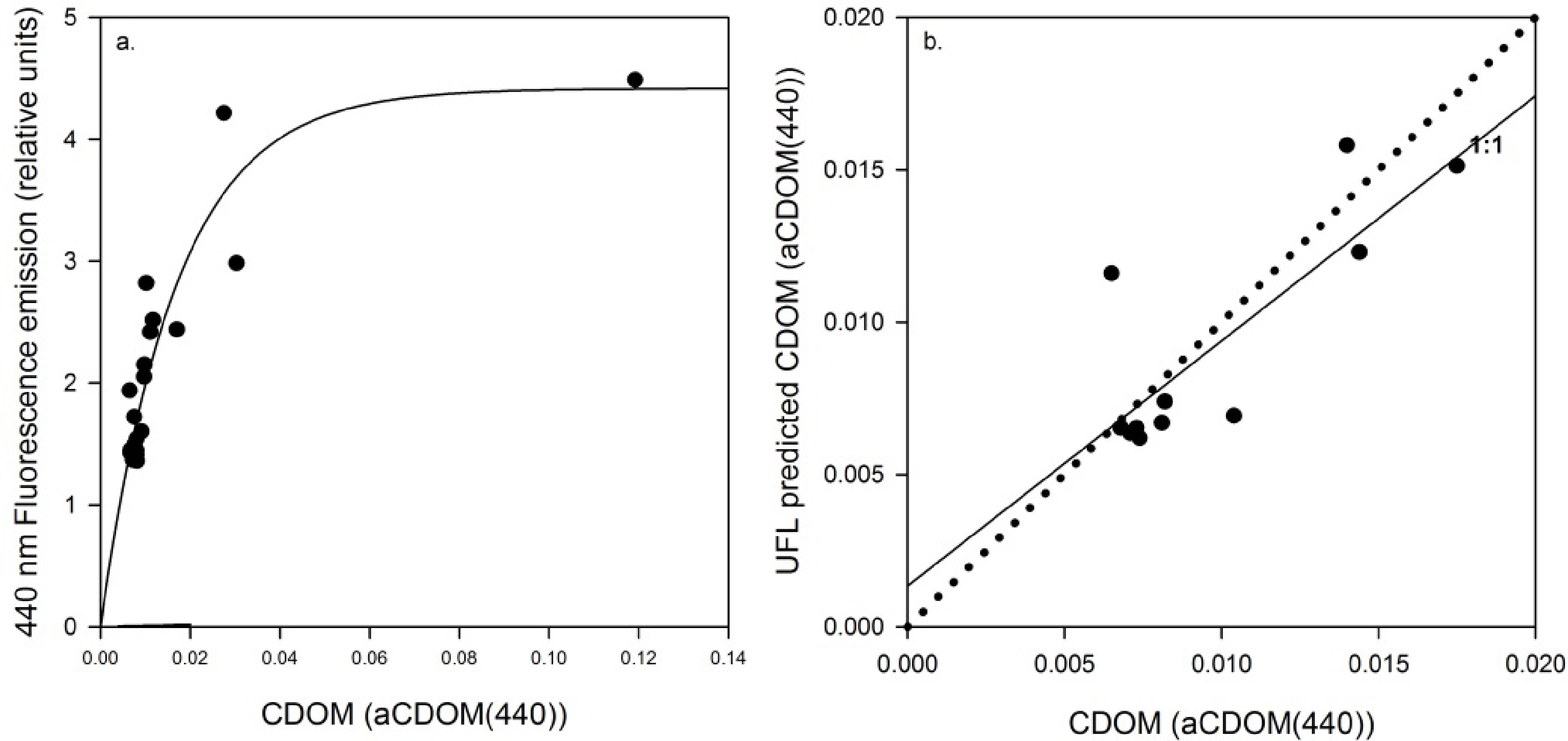
The fluorescence emission signals across the ten other UFL bands for each laboratory tank and field measurements were normalized to the Raman scattering measured at 404 nm, and relationships between normalized fluorescence at 685 nm, 440 nm, and backscattering at 355 nm and water sample chla, CDOM and TSM respectively were determined empirically. As some CDOM fluorescence can be detected at 404 nm, in addition to the more dominant signal of the water Raman scattering (Figure 2), this contribution must be removed prior the use of this band in normalization. This is accomplished through establishing a baseline between the fluorescence signals at 385 and 424 nm, related to CDOM fluorescence, and subtracting the proportionate amount from the 404 nm signal for each UFL measurement (Figure 2). Several equation models were tested for best fit. Empirical algorithms relating the UFL measurements to concentrations measured through conventional laboratory analysis were calibrated to determine specific algorithm coefficients. Field matchup data were randomly separated 70:30, for use as calibration and validation datasets respectively. Different geometries between field and laboratory setups result in differences in the fluorescence or backscattering signal to Raman scattering ratio, therefore UFL measurements in the field and in the laboratory must be calibrated separately. Regressions were performed using the statistical and graphing software, SigmaPlot v. 12.3.
4. Results
4.1. Tank Measurements
Descriptive statistics of samples analyzed by the Balaton Limnological Institute Nutrient Cycling Laboratory, coinciding with laboratory tank UFL measurements, can be found in Table 2. TSM concentrations ranged from <0.10 to 128.39 g·m−3, chla from 0.01 to 377.88 mg·m−3 and CDOM from 0.003 to 0.122 aCDOM(440). Unfortunately only 11 of the 32 laboratory tank measurement iterations resulted in valid CDOM absorbance measurements for matchup samples, due to below detection limit concentrations resulting from the short optical path (5 cm cuvette) of light in the spectrophotometer.
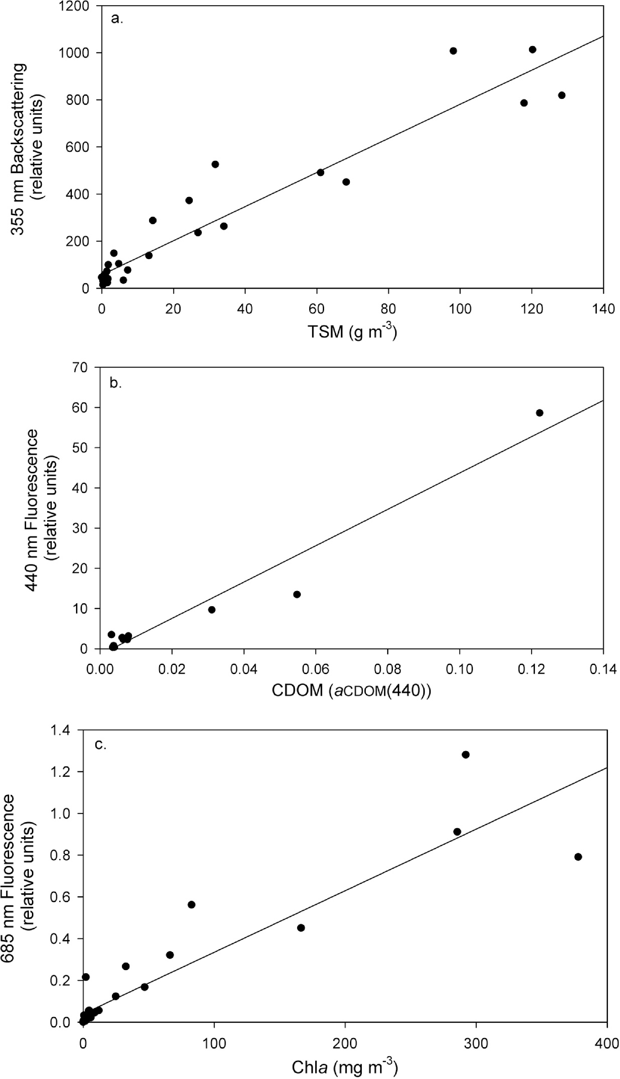
Linear models relating UFL measurements and lab-analyzed concentrations fit best for all three parameters. Pearson product-moment correlation coefficients (R), p-values and calibrated model equations can be found in Table 3. Across the full TSM concentration range, a robust model (R = 0.96, p < 0.001) was found to describe the relationship between TSM and backscattering measured from the excitation laser pulse (355 nm) (Figure 3a). A similar case was found between Raman-normalized fluorescence at 440 nm and CDOM measured by absorbance at 440 nm (aCDOM(440)) (Figure 3b; R = 0.97, p < 0.001) and between Raman-normalized fluorescence measurements at 685 nm and BLI chla measurements (Figure 3c; R = 0.92, p < 0.001).
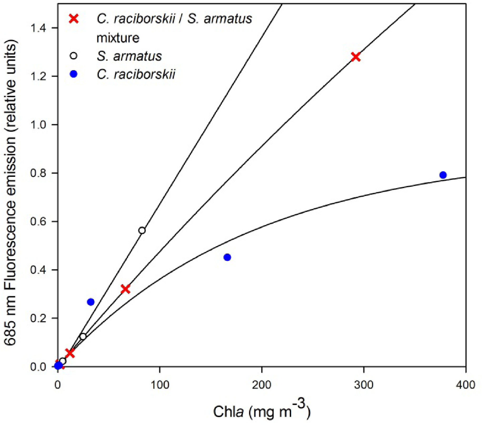
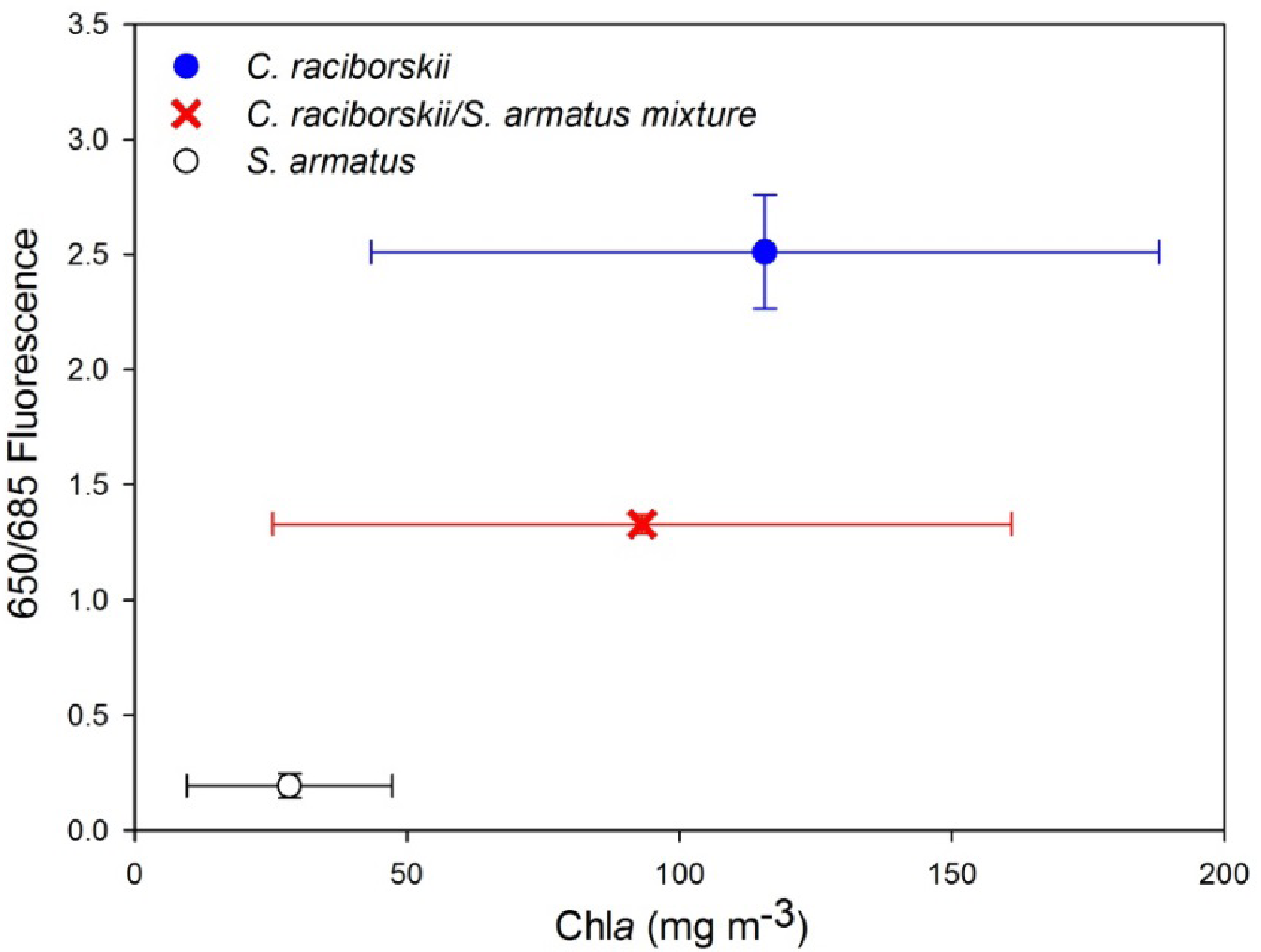
Clear and distinct relationships were found between the individual investigated algae species cultures at varying dilutions and fluorescence emission at 685 nm (Figure 4). Iterations containing dilutions of the individual cultured species S. armatus alone maintained a strong, linear relationship with fluorescence emission throughout its concentration range (1.04–82.79 mg·m−3, R = 0.99, p < 0.004, n = 4). Iterations containing only C. raciborskii were characterized by a strong, exponential growth relationship over the concentration range (0.19–377.88 mg m−3, R = 0.98, p < 0.005, n = 5). Iterations containing a mixture of the two cultures (two-thirds C. raciborskii culture, one-third S. armatus culture) were found to fall between these two end member models (Figure 4; 2.30–292.09 mg·m−3, R = 0.99, p < 0.001, n = 4).
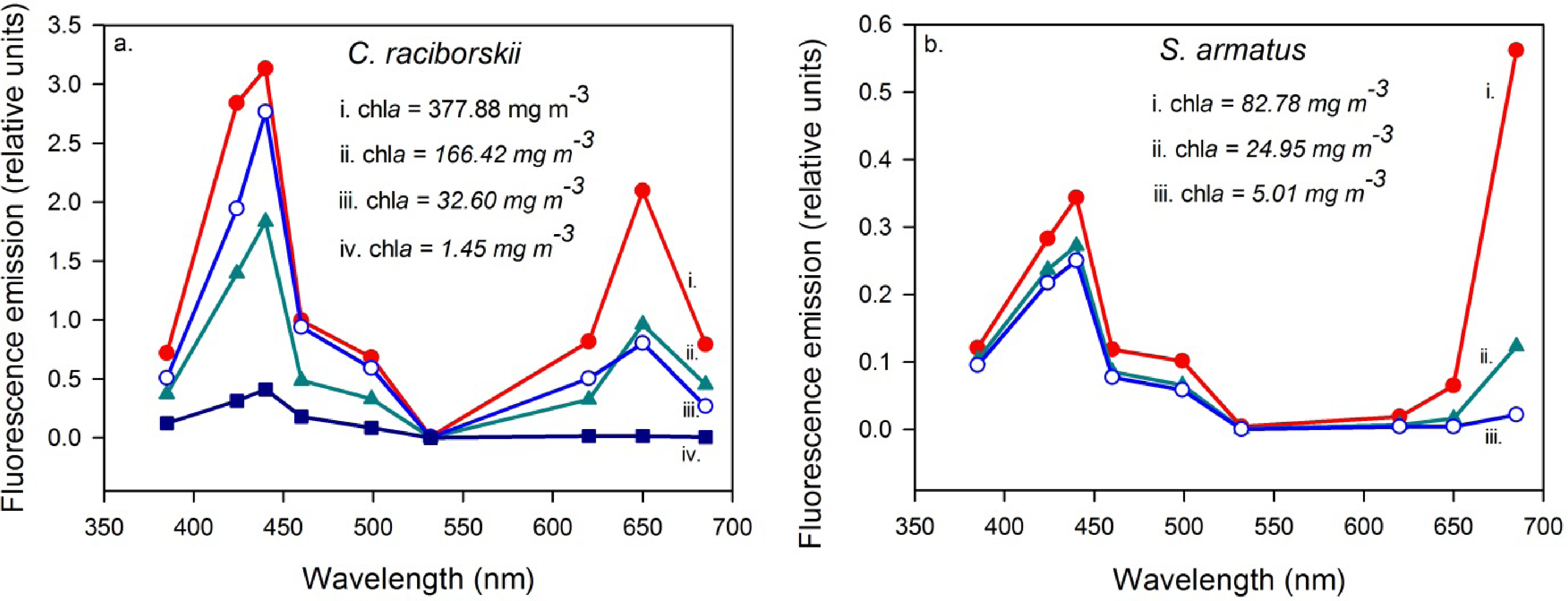
Furthermore, distinct fluorescence emissions for the two cultured species were also found to be related to the 650 nm fluorescence emission, whereby C. raciborskii is characterized by a peak at 650 nm that is absent in S. armatus (Figure 5). A Generalized Linear Model was applied, performed in RExcel, with the ratio of fluorescence emission at 650 to that at 685 as the dependent variable, and “species”, “chla concentration”, and the combined effect of “chla concentration and species” as independent variables. This identified “species” as the only significant source of variance (F = 18.68, p < 0.002), with “chla concentration” as well as “chla concentration and species” combined insignificant in the model in terms of contributed variance (F = 0.11 and 0.07, p = 0.75 and 0.93, respectively). Iterations combining the two cultures were found again to fall between the two pure culture end-members (Figure 6).
4.2. Field Measurements
Descriptive statistics of the conventional BLI laboratory matchup measurements associated with the field campaign are presented in Table 4. TSM concentrations ranged from 2.93 to 30.50 mg·m−3, largely dependent on the variable wind conditions encountered over the study period, chla from 2.66 to 7.33 mg·m−3, limited by the low productivity of Balaton between spring and summer blooms, and CDOM from 0.007 to 0.03 aCDOM(440).
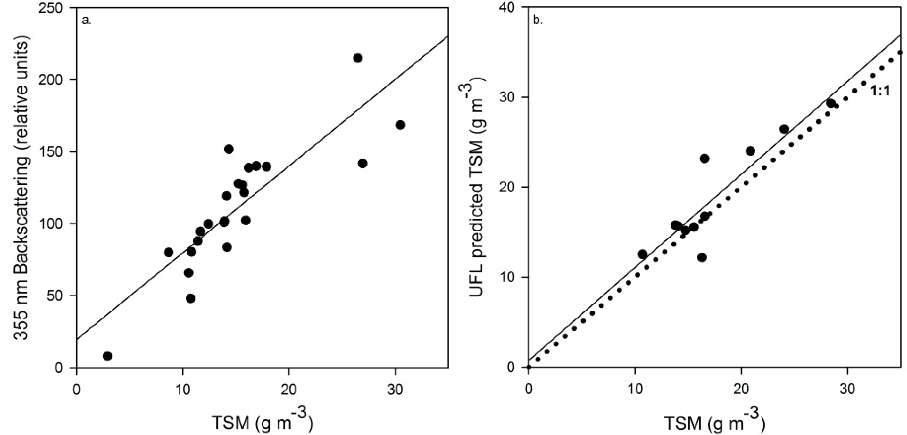
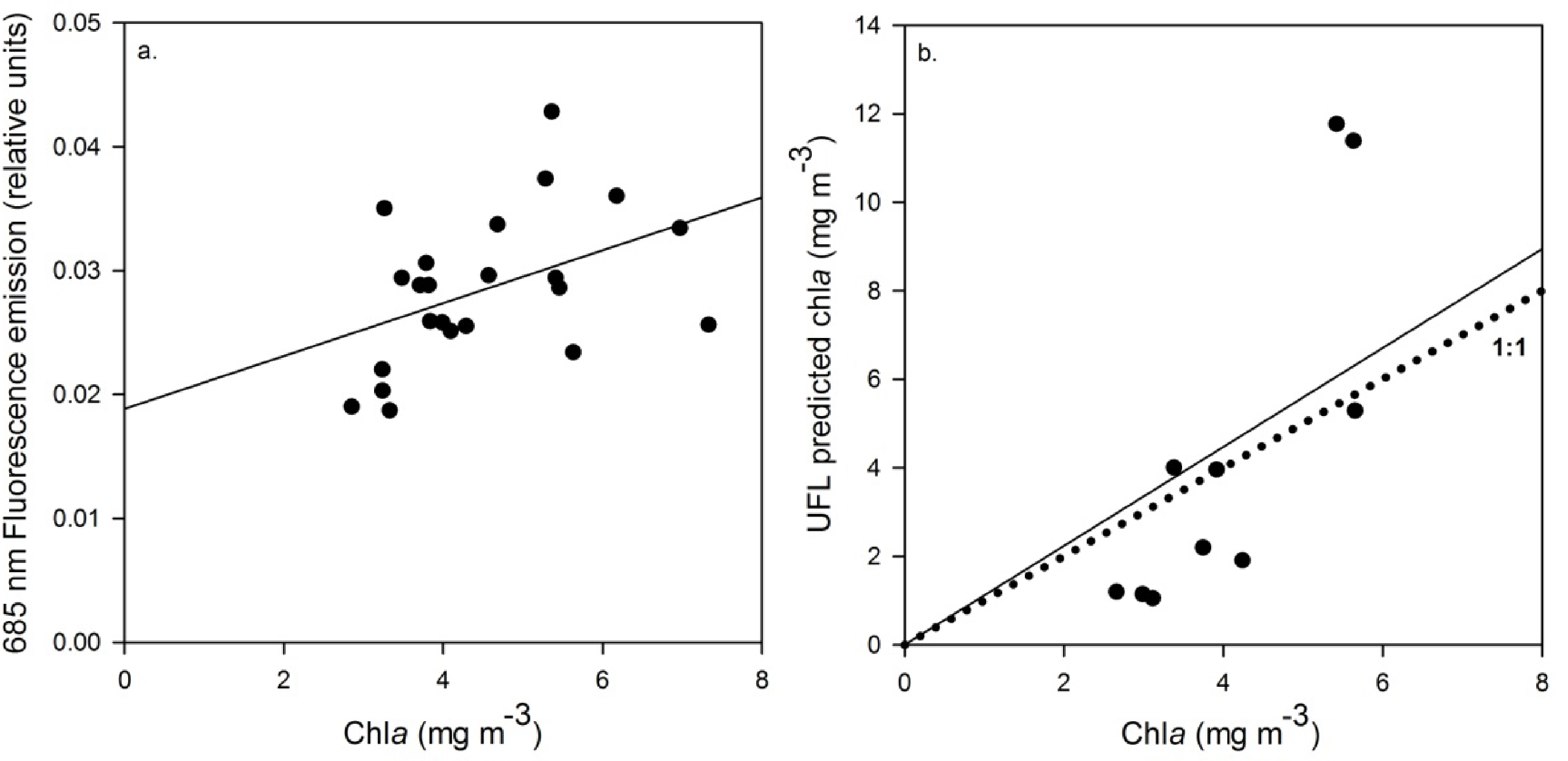
Cross-validation resulted in significant retrieval correlations, for TSM (Figure 7; R = 0.90, p < 0.001), CDOM (Figure 8; R = 0.82, p < 0.003) and chla (Figure 9; R = 0.83, p < 0.002). Table 5 presents Pearson product-moment correlation coefficients (R), p-values and calibrated model equations. The strong exponential relationship in Figure 8a likely results from some remaining error in the separation of the fluorescence from the Raman signal at 404 nm (through establishing a baseline as described in Section 3.5) in the field measurements, leading to a slight over-estimation and attribution of Raman scattering, with proportionately greater effects with higher concentrations. Attempts to account for and remove this error more fully in the raw data have been unsuccessful; nevertheless the exponential relationship of UFL measured fluorescence at 440 nm with BLI measured CDOM absorption remains strong, and can be used for reliable retrievals as seen in Figure 8b.
5. Discussion
UFL retrieval of TSM, CDOM and chla was investigated through the laboratory tank measurements and a dedicated field campaign, making use of the backscattering of the 355 nm excitation laser pulse and the chla and CDOM fluorescence emission maxima at 685 nm and 440 nm respectively. Laboratory tank measurements generally extended the concentration ranges of chla and TSM measured in the field. In field measurements, higher CDOM (0.120 aCDOM(440)) was measured in the Zala River, decreasing to 0.028–0.030 aCDOM(440) in Lake Balaton near the mouth of the Zala River, and to ≤0.02 aCDOM(440) elsewhere (Figure 1). Water from the Zala River, collected approximately 500 m upstream from its discharge into Lake Balaton, was used as the high CDOM end-member (0.122 aCDOM(440)) and diluted in the laboratory tank measurements, thus the range measured in the field was not greatly extended through the laboratory measurements. The validation of TSM was extended from concentrations greater than 2.93 g·m−3 and lower than 35 g·m−3, measured in the field, to concentrations less than 0.1 g·m−3 and exceeding 120 g·m−3, a realistic concentration range for Balaton during high wind events. As backscattering at 355 nm maintained its relationship with gravimetrically measured TSM across the full range, we have a reason to believe it can also be measured reliably during extreme events where concentrations can reach up to 130 g·m−3.
Low chla concentrations in all field measurements are a result of measurement timing, between bloom events typically characterized by high chla concentrations (≥20 mg·m−3) in the southwestern-most basin, decreasing to low concentrations (≤10 mg·m−3) in the northeastern-most basin (Figure 1). The range of chla measured in the field in the current study was extended from 2.66–7.33 mg·m−3 to 0.01–377.88 mg·m−3 through laboratory tank measurements. It was found through the manipulated tank measurements that the relationship between chla concentrations and fluorescence emissions at 685 nm varied according to the phytoplankton species investigated, for the species considered in this study. The diverging 685 nm fluorescence emission signals of the two species are likely due to variations in their chla fluorescence yield, resulting from differences in the structures and pigment contents of their respective photosystems, which is typical of different phytoplankton species. Indeed, in cyanobacteria species up to 90% of the chla pigment may be found in the non-fluorescing photosystem I (PSI), and therefore measures of extracted chla will be underestimated by the chla fluorescence maximum at 685 nm [32–35]. In comparison, chla is a more dominant photosynthetic pigment in the fluorescent photosystem II (PSII) of chlorophyta species and its extracted concentration has been related directly to fluorescence emission at or near 685 nm [20]. Although chla fluorescence yield for a species can also be affected by environmental conditions (given nutrient and light levels for example), these are not explicitly examined in or expected to influence the tank measurements, as such conditions were held constant during cultivation. This could be an important consideration when attempting similar interpretations of field measurements, however, where light and nutrient levels would be expected to be more variable.
A fluorescence maximum is found at 650 nm for the cyanobacterial species because of the dominance of the phycobilisome pigment phycocyanin (PC) in its photosystem II, which is characterized by a fluorescence maximum near this wavelength, akin to the chlorophyll a fluorescence maximum at 685 nm [20,32]. This pronounced emission maximum at 650 nm was absent in measured spectra of S. armatus, arising from its lack of PC and thus PC-related fluorescence, and the ratio of fluorescence emission at 650 nm to that at 685 nm was found to clearly and significantly distinguish the two species through UFL measurements, including mixtures of the two algal types (Figure 6).
The species tested here are common in Lake Balaton. Following these results, the extension of this analysis to the creation of a UFL-specific fluorescence emissions spectral library, including other divisions of phytoplankton (especially those with varying accessory pigments) and identification of end-member and mixture spectra is suggested, as has been done through laboratory and in vivo fluorescence spectroscopy elsewhere [20,35,36]. Quantitative analysis of other pigment concentrations, not possible during this study, would be an important component of such an exercise. This would be highly valuable so as to extend the applicability of UFL measurements, particularly with regards to transferability to other lake systems which may be dominated by species other than those characteristic for Lake Balaton. In this way the applications of UFL might be extended to distinguishing phytoplankton divisions, with a particular view to identifying the presence of species of interest, such as potentially toxic cyanobacteria, and the use of fluorescence spectroscopy to distinguish species might be evolved to be carried out using LiDAR remote sensing techniques.
In general, TSM, CDOM and chla are demonstrated through the combination of laboratory and field measurements to be reliably measured by UFL over a wide range of conditions, encountered in Lake Balaton and other lake systems, and typically not encountered in marine settings where UFL and other fluorescence LiDAR systems have been employed until now. Different concentrations and combinations of the tested parameters did not reveal any overlapping/masking or other effect that negatively affected UFL measurements, as would be expected for passive optical measurements, and so are considered applicable to at least the broad range of conditions tested here. Further testing of UFL in other lake types, such as boreal lake systems which are characterized by high DOM and strong gradients thereof, not found at Balaton, as well as highly eutrophic lakes would provide further scope and context to the measurements reported here.
6. Conclusions
The significance of the findings presented here lies in the first evaluation and demonstration of UV Fluorescence LiDAR (UFL) remote sensing for the retrieval of water quality related parameters in freshwater lakes. Chlorophyll a (chla), total suspended matter (TSM) and coloured dissolved organic matter (CDOM) were retrieved under conditions of high and variable concentrations, distinct from the marine settings where fluorescence LiDAR measurements have typically been made until now. Different algal species have been shown to have distinguishable effects on the fluorescence signals. UFL is a valuable measurement technique for sampling transects in large inland lakes at regular intervals for water quality monitoring purposes. Chla concentration as a proxy for phytoplankton biomass, and TSM and CDOM as indicators of physico-chemical lake water quality, have all been identified as key features to monitor by the Water Framework Directive of the European Commission [37] for example, which can thus be supported by UFL measurements. Application to other lake systems and explicit UFL measurement of additional algal types and of accessory pigment fluorescence is recommended.
Acknowledgments
The authors gratefully acknowledge the financial support of this project through GIONET, funded by the European Commission, Marie Curie Programme Initial Training Network, Grant Agreement PITN-GA-2010-264509. H. Balzter was supported by the Royal Society Wolfson Research Merit Award, 2011/R3. A. Zlinszky was supported by the project TÁMOP-4.2.2.A-11/1/KONV-2012-0064. Thanks also to staff of the Balaton Limnological Institute and to Thibaut Aubert for assistance in the field, and to the three anonymous reviewers for their suggestions to improve the manuscript.
Conflicts of Interest
The authors declare no conflict of interest.
References
- Farmer, F.H.; Brown, C.A., Jr.; Jarrett, O., Jr.; Campbell, J.W.; Staton, W.L. Remote Sensing of Phytoplankton Density and Diversity in Narragansett Bay Using an Airborne Fluorosensor. Proceedings of the 13th International Symposium for Remote Sensing of Environment, Ann Arbor, MI, USA, 23–27 April 1979.
- Hoge, F.E.; Swift, R.N. Airborne simultaneous spectroscopic detection of laser-induced water Raman backscatter and fluorescence from chlorophyll a and other naturally occurring pigment. Appl. Opt 1981, 20, 3197–3205. [Google Scholar]
- Barth, H.; Reuter, R.; Schröder, M. Measurement and simulation of substance specific contributions of phytoplankton, gelbstoff, and mineral particles to the underwater light field in coastal waters. EARSeL eProc 2000, 1, 165–174. [Google Scholar]
- Babichenko, S. Laser Remote Sensing of the European Marine Environment: LIF Technology and Applications. In Remote Sensing of the European Seas; Barale, V., Gade, M., Eds.; Springer: Berlin, Germany, 2008; pp. 189–204. [Google Scholar]
- Abramov, O.I.; Eremin, V.I.; Karlsen, G.G.; Lobov, L.I.; Polovinko, V.V. Application of laser ranging to determine the pollution of sea surface by oil products. Atmos. Ocean. Phys 1977, 13, 331–334. [Google Scholar]
- Barbini, R.; Colao, F.; Fantoni, R.; Palucci, A.; Ribezzo, S. Shipborne laser remote sensing of the Venice lagoon. Int. J. Remote Sens 1999, 20, 2405–2421. [Google Scholar]
- Chubarov, V.V.; Fadeev, V.V. Ecological monitoring in the Caspian Sea (mouth zone of the River Volga) with a shipboard laser spectrometer. EARSeL eProc 2004, 3, 316–322. [Google Scholar]
- Pelevin, V.N.; Abramov, O.I.; Karlsen, G.G. Subsatellite experiment in the Mediterranean Sea: a comparative study of water pollution of the seas surrounding Europe, using laser sensing from moving ship. Eng. Ecol 1995, 6, 31–41. [Google Scholar]
- Rogers, S.R.; Webster, T.; Livingstone, W.; O’Driscoll, N.J. Airborne Laser-Induced Fluorescence (LIF) Light Detection and Ranging (LiDAR) for the quantification of dissolved organic matter concentration in natural waters. Estuar. Coast 2012, 35, 959–975. [Google Scholar]
- Vodacek, A.; Hoge, F.E.; Swift, R.N.; Yungel, J.K.; Peltzer, E.T.; Bough, N.V. The use of in situ and airborne fluorescence measurements to determine UV absorption coefficients and DOC concentrations in surface waters. Limnol. Oceanogr 1995, 40, 411–415. [Google Scholar]
- Aibulatov, N.A.; Zavialov, P.O.; Pelevin, V.V. Features of hydrophysical purification Russian Black Sea coastal area near the mouths of rivers. Geoecol 2008, 4, 301–310. [Google Scholar]
- Hoge, F.E.; Lyon, P.E.; Swift, R.N.; Yungel, J.K.; Abbott, M.R.; Letelier, R.M.; Esaias, W.E. Validation of Terra-MODIS phytoplankton chlorophyll fluorescence line height. I. Initial airborne lidar results. Appl. Opt 2003, 42, 2767–2771. [Google Scholar]
- Fiorani, L.; Barbini, R.; Colao, F.; De Dominicis, L.; Fantoni, R.; Palucci, A.; Artamonov, E.S. Combination of lidar, MODIS and SeaWiFS sensors for simultaneous chlorophyll monitoring. EARSeL eProc 2004, 3, 8–17. [Google Scholar]
- Fiorani, L.; Fantoni, R.; Lazzara, L.; Nardello, I.; Okladnikov, I.; Palucci, A. Lidar calibration of satellite sensed CDOM in the southern ocean. EARSeL eProc 2006, 5, 89–99. [Google Scholar]
- Bristow, M.P.F.; Bundy, D.H.; Edmonds, C.M.; Ponto, P.E.; Frey, B.E.; Small, L.F. Airborne laser fluorosensor survey of the Columbia and Snake rivers: simultaneous measurements of chlorophyll, dissolved organics and optical attenuation. Int. J. Remote Sens 1985, 6, 1707–1734. [Google Scholar]
- Babichenko, S.; Dudelzak, A.; Poryvkina, L. Laser remote sensing of coastal and terrestrial pollution by FLS-LIDAR. EARSeL ePro 2004, 3, 1–7. [Google Scholar]
- Babichenko, S.; Dudelzak, A.; Lapimaa, J.; Lisin, A.; Poryvkina, L.; Vorobiev, A. Locating water pollution and shore discharges in coastal zone and inland waters with FLS lidar. EARSeL eProc 2006, 5, 32–41. [Google Scholar]
- Vodacek, A. Synchronous fluorescence spectroscopy of dissolved organic matter in surface waters: Application to airborne remote sensing. Remote Sens. Environ 1989, 30, 239–247. [Google Scholar]
- Anttila, S.; Kairesalo, T.; Pellikka, P. A feasible method to assess inaccuracy caused by patchiness in water quality monitoring. Environ. Monit. Assess 2008, 142, 11–22. [Google Scholar]
- Beutler, M.; Wiltshire, K.H.; Meyer, B.; Moldaenke, C.; Lüring, C.; Meyerhöfer, M.; Hansen, U.P.; Dau, H. A fluorometric method for the differentiation of algal populations in vivo and in situ. Photosynth. Res 2002, 72, 39–53. [Google Scholar]
- Stedmon, C.A.; Markager, S.; Bro, R. Tracing dissolved organic matter in aquatic environments using a new approach to fluorescence spectroscopy. Mar. Chem 2003, 82, 239–254. [Google Scholar]
- V.-Balogh, K.; Vörös, L.; Tóth, N.; Bokros, M. Changes of Organic Matter Quality along the Longitudinal Axis of a large shallow lake (Lake Balaton). Hydrobiologia 2003, 506–509, 67–74. [Google Scholar]
- Proctor, C.W.; Roesler, C.S. New insights on obtaining phytoplankton concentration and composition from in situ multispectral Chlorophyll fluorescence. Limnol. Oceanogr. Methods 2010, 8, 695–708. [Google Scholar]
- IOCCG. Remote Sensing of Ocean Color in Coastal, and Other Optically-Complex Waters; Sathyendranath, S., Ed.; Reports of the International Ocean-Color Coordinating Group, No. 3; IOCCG: Dartmouth, NS, Canada, 2000. [Google Scholar]
- Odermatt, D.; Gitelson, A.; Brando, V.E.; Schaepman, M. Review of constituent retrieval in optically deep and complex waters from satellite imagery. Remote Sens. Environ 2012, 118, 116–126. [Google Scholar]
- El-Alem, A.; Chokmani, K.; Laurion, I.; El-Adlouni, S.E. Comparative analysis of four models to estimate chlorophyll-a concentration in case-2 waters using MODerate resolution imaging spectroradiometer (MODIS) imagery. Remote Sens 2012, 4, 2373–2400. [Google Scholar]
- Mózes, A.; Présing, M.; Vörös, L. Seasonal dynamics of picocyanobacteria and Picoeukaryotes in a Large Shallow Lake (Lake Balaton, Hungary). Int. Rev. Hydrobiol 2006, 91, 38–50. [Google Scholar]
- Présing, M.; Preston, T.; Takátsy, A.; Speőber, P.; Kovács, A.W.; Vörös, L.; Kenesi, Gy.; Kóbor, I. Phytoplankton nitrogen demand and the significance of internal and external nitrogen sources in a large shallow lake (Lake Balaton, Hungary). Hydrobiologia 2008, 599, 87–95. [Google Scholar]
- Pelevin, V.N.; Abramov, O.I.; Karlsen, G.G.; Pelevin, V.V.; Stogov, A.M.; Khlebnikov, D.V. Laser sensing of surface waters of the Atlantic and the seas surrounding Europe. Atmos. Ocean. Opt 2001, 14, 704–709. [Google Scholar]
- Iwamura, T.; Nagai, H.; Ishimura, S. Improved methods for determining the contents of chlorophyll, protein, ribonucleic and deoxyribonucleic acid in planktonic populations. Int. Rev. ges. Hydrobiol. Hydrogr 1970, 55, 131–147. [Google Scholar]
- Cuthbert, I.D.; del Giorgio, P. Toward a standard method of measuring color in freshwater. Limnol. Oceanogr 1992, 37, 1319–1326. [Google Scholar]
- Beutler, M.; Wiltshire, K.H.; Arp, M.; Kruse, J.; Reineke, C.; Hansen, U.-P. A reduced model for the fluorescence from the cyanobacterial photosynthetic apparatus designed for the in situ detection of cyanobacteria. Biochim. Biophys. Acta 2003, 1604, 33–46. [Google Scholar]
- Bryant, D.A. The cyanobacterial photosynthetic apparatus: comparison to those of higher plants and photosynthetic bacteria. Can. Bull. Fish. Aquat. Sci 1986, 214, 423–500. [Google Scholar]
- Johnsen, G.; Sakshaug, E. Light harvesting in bloom-forming marine phytoplankton: species-specificity and photoacclimation. Sci. Mar 1996, 60, 47–56. [Google Scholar]
- Seppälä, J.; Ylöstalo, P.; Kaitala, S.; Hällfors, S.; Raateoja, M.; Maunula, P. Ship-of-opportunity based phycocyanin fluorescence monitoring of the filamentous cyanobacteria bloom dynamics in the Baltic Sea. Estuar. Coast. Shelf Sci 2007, 73, 489–500. [Google Scholar]
- Gregor, J.; Maršálek, B. A simple in vivo fluorescence method for the selective detection and quantification of freshwater cyanobacteria and eukaryotic algae. Acta hydrochim. hydrobiol 2005, 33, 142–148. [Google Scholar]
- European Communities. Monitoring under the Water Framework Directive. In Common Implementation Strategy for the Water Framework Directive (2000/60/EC); Guidance Document No. 7; European Communities: Luxembourg, 2003; p. 160. [Google Scholar]


| Excitation laser wavelengths | 355, 532 nm |
| Receiver spectral channels | 355, 385, 404, 424, 440, 460, 499, 532, 620, 651, 685 nm |
| Sounding frequency | 2 Hz |
| Pulse duration | 6 ns |
| Pulse energy | 1.5 mJ (355 nm pulse), 3 mJ (532 nm pulse) |
| Telescope | Kepler; adjustable length to target range 1.5–25 m |
| Power supply | 220 V, 50 Hz, 120 W |
| Dimensions; weight | 1.0 × 0.7 × 0.3 m; 35 kg |
| Receivers | Photomultipliers |
| Channel filters | Four-channel beam splitter; interference filters; high-frequency Analogue-to-Digital Conversion (ADC) |
| Telescope clear aperture | 140 mm |
| ADC frequency | 50 MHz |
| ADC resolution | 10 bit |
| n | Minimum | Maximum | Average | Median | Standard Deviation | |
|---|---|---|---|---|---|---|
| TSM (g·m−3) | 32 | <0.10 | 128.39 | 24.21 | 2.62 | 39.39 |
| CDOM (aCDOM(440)) | 11 | 0.003 | 0.122 | 0.013 | 0.007 | 0.024 |
| Chla (mg·m−3) | 32 | 0.01 | 377.88 | 44.86 | 3.31 | 96.47 |
| Equation | R | p | |
|---|---|---|---|
| TSM (g·m−3) | 7.24 × UFL355 + 57.07 | 0.96 | <0.001 |
| CDOM (aCDOM(440)) | 451.97 × UFL440 − 1.50 | 0.97 | <0.001 |
| Chla (mg·m−3) | 0.003 × UFL685 + 0.04 | 0.92 | <0.001 |
| n | Minimum | Maximum | Average | Median | Standard Deviation | |
|---|---|---|---|---|---|---|
| TSM (mg·m−3) | 34 | 2.93 | 30.50 | 15.86 | 15.01 | 5.79 |
| CDOM (aCDOM(440)) | 34 | 0.120 | 0.030 | 0.010 | 0.008 | 0.006 |
| Chla (mg·m−3) | 34 | 2.66 | 7.33 | 4.35 | 3.95 | 1.20 |
| Equation | R | RMSE (Relative) | p | |
|---|---|---|---|---|
| TSM (g·m−3) | 6.02 × UFL355 + 19.50 | 0.90 | 2.80 (16.01%) | < 0.001 |
| CDOM (aCDOM(440)) | 4.42 × (1 − exp(−59.49 × UFL440) | 0.82 | 0.0022 (22.57%) | < 0.003 |
| Chla (mg·m−3) | 0.002 × UFL685 + 0.019 | 0.83 | 0.71 (17.59%) | < 0.002 |
© 2013 by the authors; licensee MDPI, Basel, Switzerland This article is an open access article distributed under the terms and conditions of the Creative Commons Attribution license ( http://creativecommons.org/licenses/by/3.0/).
Share and Cite
Palmer, S.C.J.; Pelevin, V.V.; Goncharenko, I.; Kovács, A.W.; Zlinszky, A.; Présing, M.; Horváth, H.; Nicolás-Perea, V.; Balzter, H.; Tóth, V.R. Ultraviolet Fluorescence LiDAR (UFL) as a Measurement Tool for Water Quality Parameters in Turbid Lake Conditions. Remote Sens. 2013, 5, 4405-4422. https://doi.org/10.3390/rs5094405
Palmer SCJ, Pelevin VV, Goncharenko I, Kovács AW, Zlinszky A, Présing M, Horváth H, Nicolás-Perea V, Balzter H, Tóth VR. Ultraviolet Fluorescence LiDAR (UFL) as a Measurement Tool for Water Quality Parameters in Turbid Lake Conditions. Remote Sensing. 2013; 5(9):4405-4422. https://doi.org/10.3390/rs5094405
Chicago/Turabian StylePalmer, Stephanie C.J., Vadim V. Pelevin, Igor Goncharenko, Attila W. Kovács, András Zlinszky, Mátyás Présing, Hajnalka Horváth, Virginia Nicolás-Perea, Heiko Balzter, and Viktor R. Tóth. 2013. "Ultraviolet Fluorescence LiDAR (UFL) as a Measurement Tool for Water Quality Parameters in Turbid Lake Conditions" Remote Sensing 5, no. 9: 4405-4422. https://doi.org/10.3390/rs5094405
APA StylePalmer, S. C. J., Pelevin, V. V., Goncharenko, I., Kovács, A. W., Zlinszky, A., Présing, M., Horváth, H., Nicolás-Perea, V., Balzter, H., & Tóth, V. R. (2013). Ultraviolet Fluorescence LiDAR (UFL) as a Measurement Tool for Water Quality Parameters in Turbid Lake Conditions. Remote Sensing, 5(9), 4405-4422. https://doi.org/10.3390/rs5094405