Article

Exploring Patterns and Effects of Aerosol Quantity Flag Anomalies in MODIS Surface Reflectance Products in the Tropics

1
Department of Geosciences and Natural Resource Management, University of Copenhagen, Øster Voldgade 10, DK-1350 Copenhagen, Denmark
2
Geography Department, Humboldt-Universität zu Berlin, Unter den Linden 6, D-10099 Berlin, Germany
*
Author to whom correspondence should be addressed.
Remote Sens. 2013, 5(7), 3495-3515; https://doi.org/10.3390/rs5073495
Submission received: 18 May 2013 / Revised: 10 July 2013 / Accepted: 11 July 2013 / Published: 19 July 2013

Abstract

:
The Moderate Resolution Imaging Spectroradiometer (MODIS) has been supplying a continuous data stream since 2000, lending to detailed time series analysis of the global terrestrial environment. This paper explores a quality anomaly present in the tropics relating to the aerosol quantity flag in the daily MODIS surface reflectance products (MOD09 series) and the 16-day Vegetation Index (VI) composite products (MOD13 series) derived from the daily observations. While the anomaly is to some extent a known issue reported by the MODIS Land Quality Assessment group, very little is known about the scale of the issue, the nature and patterns of its occurrence, and potential consequences for data analysis, which explains why it is not adequately recognized throughout the literature. Two tropical regions were used to explore the anomaly and demonstrate the effects it has on the quality of selected MODIS products—one in the South American Amazon, the other in mainland Southeast Asia. The origins of the anomaly are described qualitatively in detail, and quantitative estimates of affected evergreen forest area in the MOD13A1 time series are made using blue band thresholding. The anomaly originates in the 1 km State dataset, whereby, under certain conditions, high aerosol quantity pixels are given a low aerosol quantity label, resulting in poor quality pixels with “good” quality labels. MODIS users are advised to investigate whether this anomaly has significant implications for their respective analysis and to consider the effects it may have on past studies.

1. Introduction

Polar Orbiting Environmental Satellites (POES) have been a vital component of global monitoring systems since the launch of the Advanced Very High Resolution Radiometer (AVHRR) in 1978. Since then, daily estimates of surface radiance have provided an invaluable reference of historical land cover dynamics stretching back over 30 years [1]. Following from the AVHRR era, an improved generation of Earth Observation (EO) datasets stem from the launch of a number of additional sensors, including; Système Pour l’Observation de la Terre (SPOT) VEGETATION 1 (1998) and 2 (2002); the Moderate Resolution Imaging Spectroradiometer (MODIS) on board NASA’s Terra (1999) and Aqua (2002) platforms; and the Medium Resolution Imaging Spectrometer (MERIS) from the European Environmental Satellite (ENVISAT) (2002). These new generation sensors have facilitated improved quality of EO-based mapping and time series analysis of land surface variables. Although lacking the spatial detail of higher resolution sensors, such as Landsat and SPOT, POES offer distinct advantages for monitoring larger scale vegetation processes, covering much larger areas for each pass over and supplying far superior temporal resolution, often necessary to capture near real-time abrupt events and seasonal phenological cycles.
Of the available POES datasets, the MODIS reflectance products are favored among many in the research community with a focus on monitoring regional to global vegetation dynamics. MODIS has a number of advantages when compared to other moderate-to-course resolution sensors, including superior spatial resolution (250–500 m), a broad spectral range (visible to mid-infrared), and superior geolocational accuracy [2]. One additional attraction to the MODIS dataset is the detailed description of data quality accompanying the products in the form of quality flags, including indicators of cloud cover, cloud shadow, aerosol loading and sensor-solar geometry for both the surface reflectance products (MOD09 series) [3] and the derived Vegetation Index (VI) composites (MOD13 series) [4].
One of the more common uses of MODIS reflectance data is for regional to global land cover classification [512]. Besides single date classification, a number of studies have utilized MODIS reflectance data to directly estimate land cover change [1317] or represent land cover characteristics (e.g., percent tree cover) as a continuous variable [18]. Others have used the dataset in an integrated sensor analysis, whereby MODIS is first employed as a stratification tool (for sampling-based change detection with higher resolution sensors) and, subsequently, used in regression models for spatial representation of forest area change [19,20]. A classic utility of MODIS is the assessment of vegetation change through variations of VI time series analysis [2124].
MODIS products have also been used extensively in studies focusing on phenological cycles [2527] and, more recently, for identifying breaks in trends [28], which each take a more dense time series approach. Besides using the standard VI products, others have developed innovative time series change detection methods by combining MODIS reflectance and temperature data to monitor annual disturbances [29]. However, one of the unique benefits of coupling state-of-the-art processing techniques with high temporal resolution data sources, such as from MODIS, is the ability to analyze more dense time series for near real-time change detection [30].
While most studies using MODIS data have focused on forest cover and forest cover change, a number of studies have used the MODIS time series to map regional to global agricultural area [3134] and agricultural intensification and expansion [35]. Besides various forms of land cover characterization, MODIS data has also been used to estimate carbon fluxes from vegetation [36,37] and, more recently, combined with LiDAR data to estimate biomass density [38] and carbon emissions [39] throughout the tropics.
A common theme found throughout the MODIS land surface product-based literature is an emphasis on quality screening of poor quality data. MODIS data providers actively encourage the use of the quality flags to screen out poor quality data [40], which could otherwise lead to bias in subsequent analysis. For example atmospheric contamination (cloud and aerosols) is well known to depress the Normalized Difference Vegetation Index (NDVI) [4143]. Furthermore, Samanta et al. [44] demonstrate how high aerosol loading can have a varying effect on the Enhanced Vegetation Index (EVI); suppressing EVI when blue and red reflectance increase together, but potentially inflating EVI when atmospheric scattering in the blue band is much greater than in the red, as is often the case for high aerosol loading. This phenomenon was found to be the cause of one of the major discussions in the literature regarding tropical forests response to drought. An initial study by Saleska et al. [45] showing large-scale greening of the Amazon in response to drought in 2005 was later repeated by Samanta et al. [46], with and without screening for poor quality data, and the results show the EVI greening response to be an artefact of atmospheric contamination. Samanta et al. [46] still found approximately 30% of valid data (11–12% of total drought affected area) in the drought affected forest to display dry season anomalous EVI greening, with 15% of valid data displaying browning. Samanta et al. [47] went a step further to report that the vast majority of anomalies found in the studies were found to be statistically insignificant.
These studies serve as a good example of the importance of data quality screening and the influence this can have on results and derived conclusions. However, if a step is taken further back, the importance of accurate quality data itself is recognized. Building from this crucial point, the focus of this paper will be to explore patterns and potential consequences of an anomaly originating in the MODIS quality information accompanying the daily reflectance product (MOD09GA)—namely the Aerosol Quantity Flag in the 1 km State QA dataset [3]. Correspondence with the MODIS Land Data Operational Product Quality (LDOPE) facility has confirmed the anomaly presented in the following to be a known issue (for details of known issues, explore MODIS Land QA at: http://landweb.nascom.nasa.gov/). While the anomaly can be considered somewhat recognized, very little is known about what impact it has on both surface reflectance and downstream products, i.e., the scale of the issue, under what circumstances and when and where it occurs, effects on compositing process, etc., which may explain why the anomaly seems largely unrecognized and unaccounted for in the literature and among the MODIS user community.

2. MODIS Data Products

As this paper is concerned with an anomaly present in daily reflectance and composite products, the following will present background and relevant details relating to how these products are processed and how the quality information is derived.

2.1. MOD09 Daily Land Surface Reflectance

The MOD09GA dataset is a MODIS surface reflectance product at 500 m pixel resolution for seven bands—1 (620–670 nm), 2 (841–876 nm), 3 (459–479), 4 (545–565 nm), 5 (1230–1250 nm), 6 (1628–1652 nm) and 7 (2105–2155 nm). The product is processed to level 2G, meaning radiometrically calibrated, atmospherically corrected and gridded using a sinusoidal projection. The processing for this product corrects for the effects of atmospheric gases and aerosols resulting in a band-wise estimate of surface reflectance as it would have been measured at ground level [3]. Previous to the current dataset collection, Collection 4 consisted of a number of separate level 2G surface reflectance products, including MOD09GHK (500 m surface reflectance and band quality data), MOD09GQK (250 m surface reflectance and band quality data) and MOD09GST (1 km State QA data). These datasets are now superseded by level 2G-lite products in Collection 5, resulting in a reduced number of data products, which are now contained within the MOD09GA product. Of particular importance is the 1 km State QA data held within the MOD09GA product (previously MOD09GST in Collection 4). This is considered the primary overall quality data source for MODIS surface reflectance products and is recommended for quality screening for both the 250 m and 500 m reflectance data [3]. Quality information from the 1 km State dataset also forms a central component of the compositing process for higher level downstream composite products (see below). The 1 km State QA is a 16-bit layer containing per pixel quality flags relating to cloud state, cloud shadow, aerosol quantity and basic land cover characteristics, such as the land/water, snow and fire flags. This paper is primarily concerned with the aerosol quantity flags (bits 6–7). This quality flag can take on one of four values—“Climatology” (00), “Low” (01), “Average” (10) or “High” (11). “Low” aerosol values refer to Aerosol Optical Thickness (AOT) at 550 nm less than 0.2, with “Average” between 0.2 and 0.5, and “High” greater than 0.5 [48]. “Climatology” is used when the AOT is unknown, commonly due to the presence of clouds or thick haze.

2.2. MOD13 Vegetation Indices

The MOD13 series are level 3 composite products of MODIS Vegetation Indices (VIs) derived from the daily surface reflectance MOD09 products [4]. The VIs are designed for terrestrial vegetation monitoring and are based upon absorption/reflectance patterns of visible (red and blue) and near-infrared (NIR) radiation. The most commonly used VI is the Normalized Difference Vegetation Index (NDVI), which is a normalized transformation of the NIR-to-red ratio producing values between −1 and +1 [49]. Accompanying the NDVI is the Enhanced Vegetation Index (EVI), which utilizes the difference between the blue and red reflectance to correct for atmospheric influences, along with additional parameters for removal of the canopy background signal [42]. These products come at various temporal and spatial resolutions; however, this paper is primarily focused on the 16-day composite products at 250 m (MOD13Q1), 500 m (MOD13A1) and 1 km (MOD13A2) resolutions, although the findings presented also have similar implications for the remaining MOD13 products. The compositing procedure is identical for each of these three products; however, surface reflectance in the original resolutions (250 m and 500 m) are first aggregated accordingly to suit each specific product (see Solano et al. [4] for further details). Once all 16 days of reflectance data are gathered, the compositing algorithm first screens and ranks pixels based on observation quality using the 1 km State QA dataset and viewing geometry information. Pixels that are cloud-free, have no residual aerosol contamination and a low view angle are considered the highest quality. Depending on how many of these high quality observations are available from a given 16-day period, the compositing algorithm employs one of two compositing techniques; the Constrained View angle-Maximum Value Composite (CV-MVC) or the backup Maximum Value Composite (MVC). If the number of high quality pixels is greater than or equal to two, then the two highest VI values from the group are compared, and the observation with the lowest view angle is selected to represent the 16-day period [4]. In the case where the number of available pixels is insufficient for the CV-MVC method, the backup MVC method is employed.

3. Data Used and Methods

3.1. Data Processing

The primary data sources for the analysis were the Collection 5 MODIS Terra Daily Surface Reflectance (MOD09GA) and the derived 16-day Vegetation Index composite product (MOD13A1). These datasets were downloaded from the USGS server using the MODIS Reverb tool ( https://lpdaac.usgs.gov/get_data/reverb). For each study site, four adjacent (2 × 2) MODIS tiles were chosen (South American Amazon: h11v09, h11v10, h12v09, h12v10; and mainland Southeast Asia: h27v06, h27v07, h28v06, h27v07). Tiles were mosaicked and layers extracted using the MODIS Reprojection Tool. Bit extraction for the quality data layers was done using the MODIS LDOPE tool. The native MODIS sinusoidal projection was used for data extraction and analysis; however, for presentation purposes, all maps and images are re-projected to a geographic (latitude/longitude) reference system.
Land cover was determined using the MODIS Collection 5 ‘Land Cover Type Yearly L3 Global 500 m SIN Grid’ product—MCD12Q1 [9]. The International Geosphere Biosphere Programme (IGBP) classification scheme was used to identify stable broadleaf evergreen forest pixels in both regions. This large sample of stable and relatively homogenous pixels was used for subsequent analysis (see below for details).
The MODIS Terra Level 2 Aerosol product (MOD04 L2) was used as an independent aerosol data source and was downloaded from the LAADS web interface ( http://ladsweb.nascom.nasa.gov/data/). This is a daily aerosol product produced at 10 × 10 km spatial resolution (at nadir). The Aerosol Optical Depth (or Thickness) at 550 nm layer was used for the present study.

3.2. Methods

When the aerosol anomaly occurs, visual inspection of MODIS land products and comparing these images to the accompanying quality information reveals that some of the quality information simply does not match what was represented in the image. Namely, some of the extreme high aerosol areas obvious in the images are flagged as “Low” aerosols in the corresponding quality flags. A number of tiles were visually inspected to explore the nature of the problem, an example of which will be given to introduce the issue in the results section.
Although the anomaly is found to originate in the daily 1 km State data, the error is inherited by the downstream composite products derived from this dataset. To investigate how the aerosol anomaly affects the selection of pixels in the compositing process, a stack of 16 daily images from the MOD09GA product was examined for two composite periods in the MOD13A1 product—one in each study region. A detailed look at the composite pixel selection for a single pixel in each study region illustrates well how the aerosol mislabeling manifests itself in the quality of the time series. For each day in the selected 16-day periods, reflectance data were converted to daily NDVI and EVI, view angle data were extracted and corresponding aerosol quality flags (bits 6–7) were extracted from the 1 km State layer. To reveal which of these daily observations was selected by the compositing algorithm, the VI values were then ranked from highest to lowest and compared to the corresponding VI values chosen by the MOD13A1 compositing algorithm. After showing that the MOD13A1 pixel is mistakenly chosen, the “pixel that should be chosen” is identified using the same selection criteria outlined in the MOD13 series user manual [4].
To estimate the area affected by the aerosol anomaly and to identify which periods in the MOD13A1 time series were prone to it, a methodology based upon a simple, yet robust, thresholding of blue band reflectance was developed. For consistency in the analysis and to limit the influence of land cover change, the region of interest was limited to broadleaf evergreen forest using the MCD12Q1 product (IGBP classification). Although some extensive patches of mixed deciduous forest can be found throughout Southeast Asia, the broadleaf evergreen forest class was the overwhelmingly dominant class in both regions. Only pixels that were consistently classified as broadleaf evergreen forest for each year from 2001 to 2009 (2010 and 2011 data are unavailable) were included in the analysis. Under low aerosol conditions, blue band reflectance for evergreen forest is typically very low (<2%), even in the dry season, as most of this light is absorbed for photosynthesis. In contrast, when high aerosols are encountered, blue band reflectance increases substantially, due to atmospheric scattering. When the aerosol anomaly occurs in a given tile, a fraction of the image may have evergreen forest correctly labelled as “Low” aerosols, while the anomaly affected fraction will have been incorrectly labelled as “Low” aerosols, despite these pixels being badly contaminated by high aerosol loading. The blue band reflectance threshold was therefore determined by examining the histograms of the affected tiles using a combined “broadleaf evergreen forest/low aerosol” mask. Such a histogram will have two very distinctive peaks. The first peak will be for evergreen forest with correct aerosol quality information. These pixels are tightly distributed below 2–3% blue reflectance. The second peak will represent evergreen forest that has been incorrectly labelled as “low” aerosols, with blue reflectance typically above 10%. Evergreen forest pixels with a “Low” aerosol quality flag and blue band reflectance above 10% were therefore considered erroneous. This threshold is considered robust, because of the very distinctive groups evident in the histogram, with comparably very low counts of pixels found between the groups.
For further details on each quality layer used throughout the paper (e.g., 1 km State—Aerosol Quantity (bits 6–7)) refer to Vermote et al. (Table 16 in [3]) and Solano et al. (Table 5 in [4]) for the MOD09GA and the MOD13A1 products, respectively.

4. Results

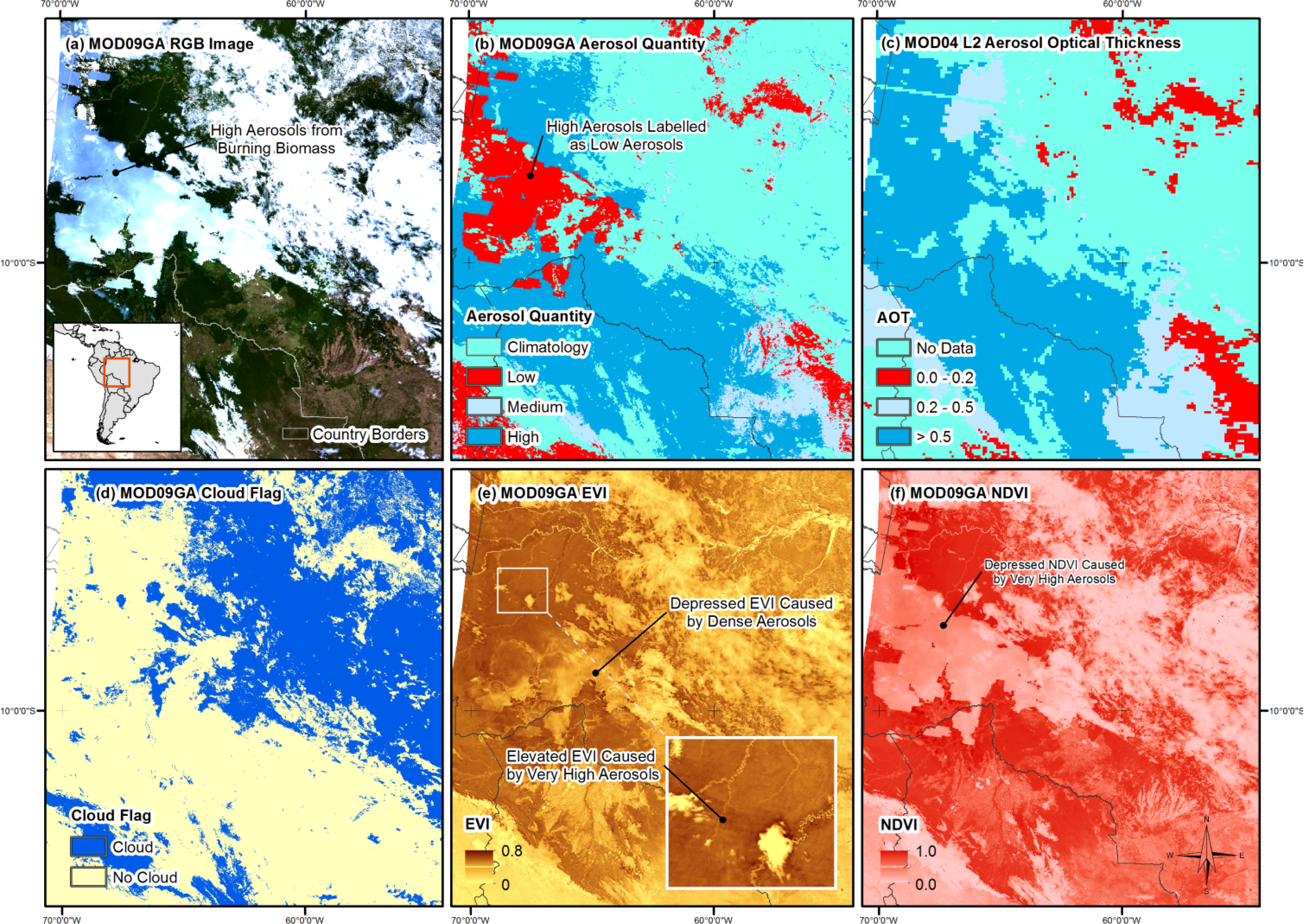
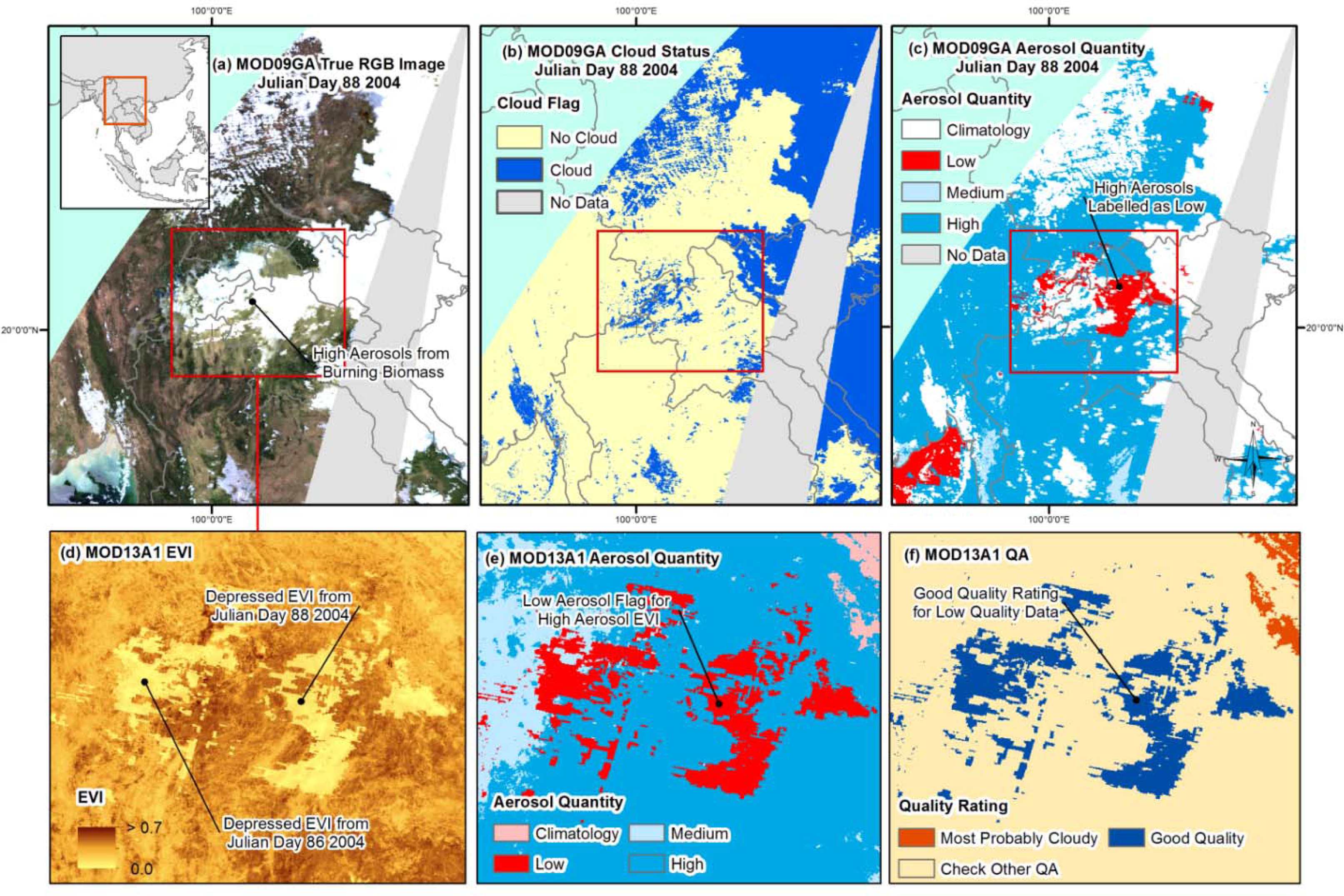
4.1. Description of the Anomaly

The following section presents a typical example of the anomaly that can be found in both study regions. This example serves to provide a qualitative assessment of the origins of the anomaly and its implications for the surface reflectance, EVI and NDVI. Figure 1a shows a true color image from the four MOD09GA tiles in the Amazon region.
The dry season in the region usually lasts from July to September. The image presented was captured towards the end of the dry season on 2 September 2003 (Julian day 245), this specific time of the year being well known for high aerosol contamination originating from biomass burning [5052]. A very large plume of what the authors believe to be very high aerosols can be observed stemming from the center of the image and dispersing westwards from Brazil towards eastern Peru and Columbia. Figure 1b shows the aerosol quantity layer from the MOD09GA 1 km State dataset (bits 6–7) for the same day in question. This image illustrates that nearly the entire extreme high aerosol area is labelled incorrectly as “Low” aerosols, with a smaller fraction labelled as “Climatology”.
When the aerosol quantity layer in Figure 1b is compared to the aerosol optical depth from the MOD04 L2 product in Figure 1c, it can be seen that while the problem area consisting of extreme high aerosol loading is labelled incorrectly in the MOD09GA product, labels outside the problem area follow similar patterns in both images and can, therefore, be considered trustworthy. Figure 1d shows the Internal Cloud Flag from the 1 km State data (bit 10). Some of the extreme aerosol area is flagged as cloud in this layer, which seems to be areas closer to the aerosol source. In the example presented, the area of concern is large and relatively homogenous, and the anomaly is, therefore, quite obvious. However, the problem has also been found to occur in much smaller isolated groups of pixels, usually located between areas of thin and patchy cloud cover. In these instances, the anomaly seems to be caused by thin cloud remnants, rather than extreme aerosol loading.
Figure 1e,f show the effect that the problem area aerosols have on EVI and NDVI values, respectively. While the NDVI response is an all-round suppression of values, as expected, the EVI behaves in a more dynamic manner. EVI values are suppressed where the aerosols are more dense (possibly closer to the aerosol source), while the values become artificially inflated as the aerosols become more dispersed (see inset in Figure 1e).

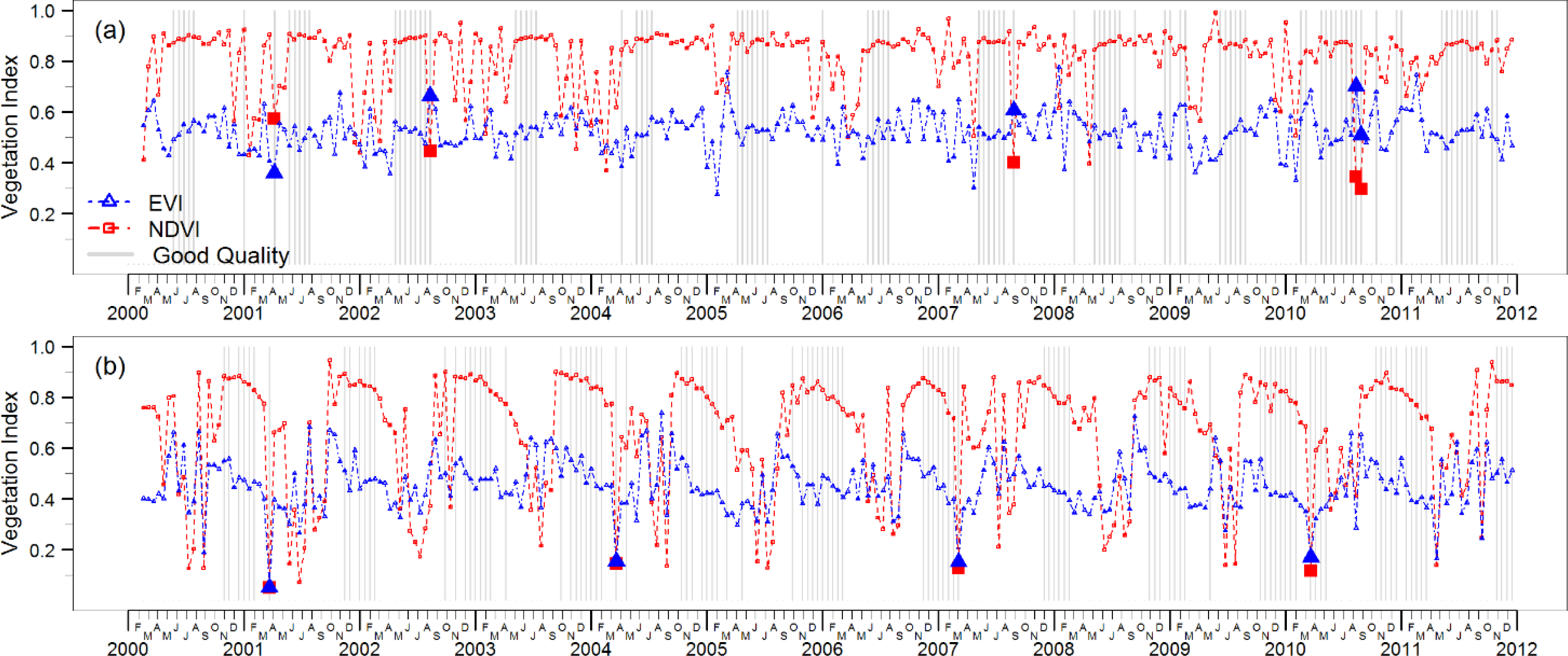
4.2. Effects on Composite Products

Since this quality information from the daily data (the 1 km State dataset) streams directly into the VI composite processing chain (MOD13 series), the anomaly will inevitably manifest itself in these downstream products. Figure 2a shows a true color image from the four tiles over mainland Southeast Asia (MOD09GA product). Figure 2b,c shows the corresponding Internal Cloud Flag (bit 10) and the aerosol quantity information (bits 6–7) from the 1 km State layer, respectively. The dry season in this region usually runs from November to March/April. This image is captured in the late dry season on 28 March 2004 (Julian day 088). Similar to the Amazon region, this particular time of year is notorious for widespread fire activity, whereby many of the shifting cultivators make final preparations to their plots for the upcoming growing season [5355]. In this case, an extreme high aerosol area is evident over northern Laos, a landscape overwhelmingly dominated by shifting cultivation. Figure 2c again shows how the problem area where high aerosols are present is labelled as either “Low” aerosols or “Climatology”. A smaller fraction of the area in question is labelled as cloud in Figure 2b. Figure 2d shows EVI values from the 500 m 16-day composite product (MOD13A1) from the indicated subset over northern Laos. For this specific composite image, the compositing algorithm selects the best quality pixel from all MODIS Terra observations from Julian Day 081 to 096. Figure 2e shows the aerosol quantity (bits 6–7 of the VI Quality layer) and Figure 2f shows the corresponding MODLAND QA (bits 0–1 of the VI quality layer) for the same subset. The EVI values are clearly depressed in the areas labelled as “Good Quality” and “Low” aerosols. The “Day of the Year” layer allows the user to track which Julian day each pixel was taken from. The majority of the incorrectly labelled pixels have come from Julian day 088—originating from the extreme high aerosol affected region from the images displayed in Figure 2a–c. Similar anomaly-affected data from other days within the compositing period have also been selected in the composite image.
Table 1 shows a more detailed insight into how individual pixels are selected by the MOD13A1 compositing algorithm and how the aerosol anomaly described can cause poor quality data to be picked instead of optimal VI values. Table 1a is an example from the Southeast Asian context and takes a selected pixel from the same area and time period depicted above in Figure 2c. Because the compositing algorithm favors low aerosol data, the solitary low aerosol observation (which, as shown in Figure 2, is an incorrect aerosol label) from Julian day 088 is chosen for the composite image, causing extremely suppressed EVI (0.15) and NDVI (0.14) values. If the anomaly was not present, however, the chosen observation would be labelled as “High” aerosol or “Climatology”, and the best quality pixel would now come from Julian day 094; cloud free observation, “Average” aerosol quantity, relatively low view angle and producing EVI and NDVI values of 0.39 and 0.64, respectively. Table 1b shows an example from the Amazonas region from the sixteenth composite period of 2003 (Julian day 241 to 256). The observation chosen by the compositing algorithm was also selected from an extreme high aerosol anomaly area on Julian day 249, with an incorrect “Low” aerosol label. Here, the varied effects that high aerosols can have on the different VI values can be seen—EVI being inflated (0.69) and NDVI being suppressed (0.44). If the aerosol labels were accurate, then the pixel that should be chosen for the composite would be from Julian day 254; cloud free observation, “Average” aerosol quantity, near nadir view angle and giving EVI and NDVI values of 0.55 and 0.84, respectively.
At the pixel level, these errors can have a considerable effect on the MODIS VI time series. Figure 3a,b shows a single pixel time series from each study region for NDVI and EVI, with “good quality observations” (from the MODLAND_QA bits) indicated by the vertical grey lines. The Amazonas case (Figure 3a) comes from a stable evergreen forest pixel in northeast Bolivia. It can be seen that the error has occurred five times throughout the time series (highlighted symbols; wet season—2001, dry season—2002, 2007, 2010 × 2). In each of these cases, the concerned observations are labelled as “good data”, yet have severely suppressed NDVI values. The EVI behaves in a more erratic manner, whereby three out of the five times that the error occurs, the EVI is artificially inflated. The other two times that the error occurs, the blue band correction in the EVI calculation seems to deal more effectively with the high aerosol loading. The Southeast Asian pixel comes from a stable forest region in northern Laos (Figure 3b). Here, it can be seen that the error occurs four times throughout the time series (highlighted symbols; dry season—2001, 2004, 2007, 2010), whereby the VI values are depressed and mislabeled as “good data”. This pixel has also been taken from a stable evergreen forest class throughout the MCD12Q1 series, indicating no land cover clearing during this period.

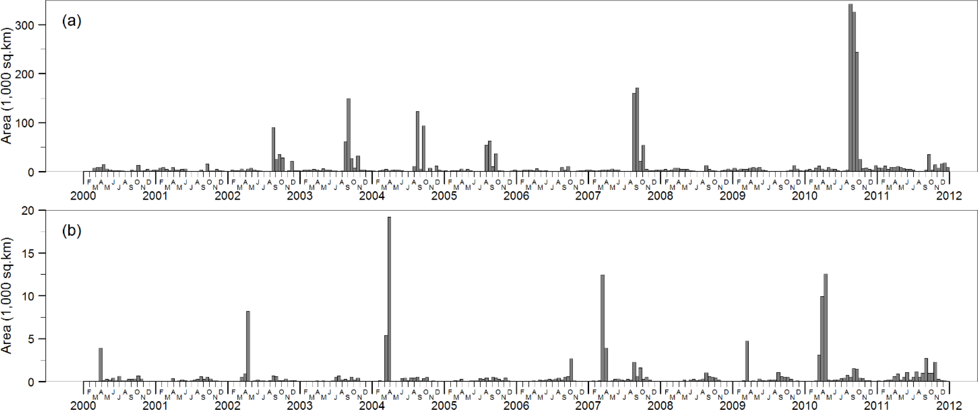
4.3. Area Affected by the Anomaly

Figure 4a,b shows the estimated stable evergreen forest area affected by the aerosol error for each 16-day composite period for the four tiles over the Amazon region and four tiles over mainland Southeast Asia, respectively, from February 2000 to December 2011. The figures reveal that not only a substantial amount of the composite periods are considerably affected, but that the area affected can be quite large, depending on the season and individual year. The larger spikes are generally confined to the late dry season in each region—August to October in the Amazon region and mid-February to late April in mainland Southeast Asia. However, there are some notable lower magnitude spikes during the August to October periods in mainland Southeast Asia. The smaller bars between the dry seasons are accounted for by the anomaly occurring in high aerosol or cloud remnant spaces often located between areas affected by patchy cloud cover. Although significant areas are affected in both regions, it is obvious that the scale of the problem is more acute in the Amazon region compared to mainland Southeast Asia. In the Amazon study region, an estimated 1,754,700 km2 of stable evergreen forest (62%) has been affected at least once by the error throughout the entire time series. In general, the most badly affected areas (multiple occurrences) were located closer to the forest edge, where most of the clearing and burning occurs. An estimated 861,600 km2 (30%) has been affected at least twice by the error, with some of the hotspot areas affected over five times throughout the time series. 2010 was by far the most badly affected year, with an estimated 869,300 km2 (30%) affected—some areas multiple times. In the mainland Southeast Asia region, it was estimated that 111,135 km2 (24%) of stable evergreen forest are affected at least once by the error. The vast majority of the affected area lies in northern Laos and eastern Myanmar, and these are also the areas that frequently experience multiple occurrences throughout the time series. The worst affected year was in 2004, with a total of 26,170 km2 (5.7%) of evergreen forest suffering from corrupted data in the study region.

5. Discussion

5.1. Products and Regions Affected by the Anomaly

The analysis has focused on the current MODIS collection, Collection 5. For consistency, this paper has focused on the MOD09GA surface reflectance product and the MOD13A1 product, both provided by MODIS Terra with 500 m pixel resolution. The authors have also studied the MOD13Q1 (250 m VI) and MOD13A2 (1 km VI) products and have found the anomaly to also be present, which is intuitive, as they both use the 1 km State data as input for their respective compositing algorithm. Indeed, each MODIS product dependent on the 1 km State aerosol quantity bits are likely to be somewhat affected by the anomaly. Although this analysis is focused solely on MODIS Terra datasets, further investigations show the anomaly to be present in MODIS Aqua versions of the concerned products; however, as of yet, a thorough investigation has not been performed on the Aqua datasets.
The anomaly has been explored using two case study sites in the tropics—the Amazonas and mainland Southeast Asia. The authors have also been working the same datasets on Insular Southeast Asia and have found similar patterns to be present. It is, therefore, most likely a global issue, but the anomaly is also likely more prominent in parts of the globe characterized by high aerosol loading [56] originating from seasonal combustion of biomass [57], associated with both human land-use activities and naturally occurring wildfires. Such areas include large parts of North America, central and southern Africa, south Asia and northern Australia.
The MODIS Land Product Quality Assessment group actively encourages feedback from the MODIS user community regarding product quality issues, which are investigated by the team and posted as known issues on the MODIS Land Quality Assessment website. This, in turn, acts as important input for future improvements to MODIS datasets, which is evident in each progressive collection. Following the MODIS ethos, the authors have been in correspondence with the MODIS Land Data Operational Product Quality (LDOPE) facility, who have confirmed the anomaly presented in this paper to be a known issue in past collections, but which should be thankfully resolved in the upcoming Collection 6, due for release.

5.2. Uncertainties

Throughout this paper, the presented examples are regularly referred to be caused by very high aerosol loading originating from biomass burning. However, in Section 5.1, it is also mentioned that the problem was also found to occur in much smaller isolated groups of pixels, usually located between areas of thin and patchy cloud cover. While there is scope to argue that the presented examples of the anomaly (e.g., Figures 1 and 2) may originate from the mislabeling of cloud, the evidence presented here makes for a strong case that the observed seasonal patterns of the anomaly are stemming from aerosols, i.e., mainly well-known times of intense aerosol release in both regions consistently correspond to peaks in the area affected by the anomaly (Figure 4). Outside of these intense aerosol release periods (August–October in the Amazon, March–April in mainland Southeast Asia), it may be residual cloud, which accounts for the remaining area affected in Figure 4. It should be noted that parts of areas affected by the extreme aerosol loading, as seen in Figure 1 and Figure 2, are sometimes flagged as cloud or mixed cloud in the 1 km State dataset (Cloud State (bits 0–1) and the Internal Cloud Flag (bit 10).
The estimated area of evergreen forest affected by the anomaly presented in Figure 4 is based upon thresholding of the blue band included in the MOD13A1 product. Based upon a relatively straightforward procedure, this method was considered to be very robust for separating the two distinctive classes in question, i.e., clear-sky evergreen forest with blue band reflectance normally below 2–3% vs. evergreen forest affected by the high aerosol anomaly with blue band reflectance typically above 10%. As evergreen forest rarely displays blue reflectance above 4–5%, pixels between this upper level and the 10% threshold applied may also have been affected by the aerosol flag anomaly. For this reason, the area estimate can be considered slightly conservative. Additionally, the influence of forest clearings that cause high blue reflectance from exposed soils was minimized by focusing the analysis on stable evergreen forest only.

5.3. Implications for Research

The implications that the anomaly will have on research regarding land cover monitoring are varied, depending on the specific methodology and objectives of each study. Often, course resolution reflectance data is used for broad-scale land cover classification [7,14,58,59]. In such large-scale analysis, the pre-processing stage will almost always involve some form of image compositing, which requires pixel quality screening to minimize the undesired effects of cloud, aerosols and viewing geometry. If the MODIS QA flags are used for the screening process, poor quality data will be included in the compositing process, which will inevitably lead to lower accuracy in the affected regions. Similarly, if misleading aerosol flags are used to select only ‘good quality’ pixels for the change detection using MODIS VIs, considerable errors of commission will be present, where VI values have been artificially suppressed by aerosol contamination. The problem is compounded by the fact that most studies in the tropics target the dry season for data acquisition, largely because it is the only window in the year where cloud-free observations can be attained; yet, this is also the period where the aerosol error has its greatest impact.
The MODIS VI time series has been used extensively to monitor vegetation phenological trends [24,25,27,28]. Often, noisy VI data are filtered and/or interpolated to reduce the effects of bad quality or missing data [60,61]. For example, Timesat [62] offers a number of smoothing functions to process noisy time series. One of the advantages of such software is that good quality observations can be given higher weight in the smoothing process. In this way, higher quality data will have a greater influence on the shape of the fitted function compared to lower quality data. By introducing suboptimal VI values and poor quality flag information, as demonstrated in the analysis above, the weight is given to poor quality data, resulting in skewed fitted functions and bias estimates of vegetation phenology signals.
Regarding the debate continuing in the Amazonas in relation to drought and EVI greening, although Samanta et al. [44,46,47] and others [63] stress the importance of using the MODIS quality flags for screening corrupt data from the analysis, these papers make no reference to the aerosol anomaly described in the current paper. If the anomaly has been unaccounted for in these studies (as is possible with many other studies), poor quality data may have been unintentionally included in the analysis. It is impossible to say, however, what impact this would have on the overall results, but it would certainly reduce the amount of valid pixels for analysis and have varying effects on EVI values. As shown in Figure 1e and Figure 3a,b, the aerosol error can cause EVI values to behave erratically, sometimes depressed, sometimes elevated and sometimes seemingly unaffected (due to the atmospheric correction component of EVI formulation), introducing a varying bias to the time series, which can be especially prominent in the dry season.

5.4. Alternative Quality Screening Approaches

A number of studies have developed alternative methods for quality screening, working independent of the supplied MODIS QA data. For example, [64] presented a simple, yet effective, method for masking cloud and aerosols in Southeast Asia based upon reflectance properties of MODIS bands 1, 3 and 7. Although this method was originally designed for image compositing focused on burned area detection, it has been shown to be useful in other studies concerned with land cover classification [8,14]. Similar methods could be employed to screen out the erroneous data identified in this paper.
One of the more recent advances in MODIS reflectance quality comes from Multi-Angle Implementation of Atmospheric Correction (MAIAC) algorithm [65,66]. MAIAC uses a new cloud screening technique, together with innovative aerosol retrieval and atmospheric correction procedures. MODIS data processed using MAIAC has shown significant improvements compared with the current MODIS surface reflectance and VI composite products [67]. This new generation atmospheric correction algorithm boasts noise level reduction by a factor of up to 10, improves cloud detection and has considerable increases in could-free pixels, meaning an overall reduction in uncertainty promised for future satellite-based vegetation monitoring.

6. Conclusion

The analysis explores the patterns and effects of aerosol quality flag anomalies inherent in a number of Collection 5 Moderate Resolution Imaging Spectroradiometer (MODIS) land surface products (MOD09GA, MOD13 series). The findings presented have not previously been mentioned throughout the relevant literature and, therefore, have implications for both past and future use of the related Collection 5 datasets. Using two study sites in the tropics—one in the South American Amazon, the other in mainland Southeast Asia—the study has found that under certain atmospheric conditions, whereby aerosol loading is extremely high, the methods for determining aerosol quantity for the daily MODIS 1 km State dataset fails and erroneously labels the affected high aerosol pixels as low. The analysis goes further to demonstrate how this anomaly manifests itself in downstream MODIS products that use the daily 1 km State dataset as input for image compositing, causing suboptimal pixels to be chosen by the compositing algorithm and giving these pixels a high quality rating, for poor quality data. Using the MOD13A1 dataset (years 2000–2012) to explore in more detail, an estimated 62% of evergreen forest was found to be affected at least once by the anomaly in the Amazon region, compared to 24% affected in the mainland Southeast Asia region. This analysis has also found a distinct reoccurring pattern, whereby the vast majority of the area affected by the anomaly occurs in each respective regions’ dry season, providing strong supporting evidence that these peaks are linked to the presence of very high aerosol loadings caused by seasonal biomass burning. The aerosol effect on most commonly used Vegetation Indices is varied, causing the Normalized Difference Vegetation Index (NDVI) to be depressed and the Enhanced Vegetation Index (EVI) to behave erratically, showing a range of unaffected, depressed and inflated values. The behavior of EVI, in particular, coupled with the high quality rating given to the affected data, contributes an interesting perspective to the current discussion of tropical forest monitoring, especially in the Amazonas region. Considering the findings presented in this paper, the MODIS community should be cautious when using the affected products, especially when using dry season Vegetation Indices in respective analyses and, more so, in regions known for extreme aerosol loadings originating from burning biomass. If the data is used, an additional quality screening step should be considered, so as to minimize the amount of corrupt pixels in the analysis. Looking forward, MODIS Collection 6 promises improved quality screening, which should ultimately reduce this form of bias in the respective datasets. Often, it is assumed by users that highly processed datasets, such as MODIS products, are more or less immune to such errors and are used without critical exploration prior to the analysis. The reality is that remotely sensed data and derived products will always be prone to such errors and, ultimately, it is the users’ responsibility to scrutinize each data set before progressing forward.

Acknowledgments

This research is part of the research project entitled, Impacts of Reducing Emissions from Deforestation and Forest Degradation and Enhancing Carbon Stocks (I-REDD+). I-REDD+ is funded by the European Community’s Seventh Framework Research Programme. More information can be found at: www.i-redd.eu.

Conflict of Interest

The authors declare no conflict of interest.

References

  1. Tucker, C.J.; Pinzon, J.E.; Brown, M.E.; Slayback, D.A.; Pak, E.W.; Mahoney, R.; Vermote, E.F.; El Saleous, N. An extended AVHRR 8-km NDVI dataset compatible with MODIS and SPOT vegetation NDVI data. Int. J. Remote Sens 2005, 26, 4485–4498. [Google Scholar]
  2. Wolfe, R.E.; Nishihama, M.; Fleig, A.J.; Kuyper, J.A.; Roy, D.P.; Storey, J.C.; Patt, F.S. Achieving sub-pixel geolocation accuracy in support of MODIS land science. Remote Sens. Environ 2002, 83, 31–49. [Google Scholar]
  3. Vermote, E.F.; Kotchenova, S.Y.; Ray, J.P. MODIS Surface Reflectance User’s Guide; MODIS Land Surface Reflectance Science Computing Facility; NASA: College Park, MD, USA, 2011; pp. 1–40. [Google Scholar]
  4. Solano, R.; Didan, K.; Jacobson, A.; Huete, A. MODIS Vegetation Index User’s Guide (MOD13 Series); Collection 5; Vegetation Index and Phenology Lab, The University of Arizona: Tucson, AZ, USA, 2010. [Google Scholar]
  5. Wessels, K.; De Fries, R.S.; Dempewolf, J.; Anderson, L.O.; Hansen, A.J.; Powell, S.L.; Moran, E.F. Mapping regional land cover with MODIS data for biological conservation: Examples from the Greater Yellowstone Ecosystem, USA and Para State, Brazil. Remote Sens. Environ 2004, 92, 67–83. [Google Scholar]
  6. Sedano, F.; Gong, P.; Ferrao, M. Land cover assessment with MODIS imagery in southern African Miombo ecosystems. Remote Sens. Environ 2005, 98, 429–441. [Google Scholar]
  7. Carrão, H.; Gonçalves, P.; Caetano, M. Contribution of multispectral and multitemporal information from MODIS images to land cover classification. Remote Sens. Environ 2008, 112, 986–997. [Google Scholar]
  8. Miettinen, J.; Shi, C.; Tan, W.J.; Liew, S.C. 2010 land cover map of insular Southeast Asia in 250-m spatial resolution. Remote Sens. Lett 2012, 3, 11–20. [Google Scholar]
  9. Friedl, M.A.; Sulla-Menashe, D.; Tan, B.; Schneider, A.; Ramankutty, N.; Sibley, A.; Huang, X. MODIS Collection 5 global land cover: Algorithm refinements and characterization of new datasets. Remote Sens. Environ 2010, 114, 168–182. [Google Scholar]
  10. Xiao, X.; Biradar, C.M.; Czarnecki, C.; Alabi, T.; Keller, M. A simple algorithm for large-scale mapping of evergreen forests in tropical America, Africa and Asia. Remote Sens 2009, 1, 355–374. [Google Scholar]
  11. Clerici, N.; Weissteiner, C.J.; Gerard, F. Exploring the use of MODIS NDVI-based phenology indicators for classifying forest general habitat categories. Remote Sens 2012, 4, 1781–1803. [Google Scholar]
  12. Hüttich, C.; Gessner, U.; Herold, M.; Strohbach, B.J.; Schmidt, M.; Keil, M.; Dech, S. On the suitability of MODIS time series metrics to map vegetation types in dry savanna ecosystems: A case study in the Kalahari of NE Namibia. Remote Sens 2009, 1, 620–643. [Google Scholar]
  13. Zhan, X.; Sohlberg, R.A.; Townshend, J.R.G.; DiMiceli, C.; Carroll, M.L.; Eastman, J.C.; Hansen, M.C.; DeFries, R.S. Detection of land cover changes using MODIS 250 m data. Remote Sens. Environ 2002, 83, 336–350. [Google Scholar]
  14. Langner, A.; Miettinen, J.; Siegert, F. Land cover change 2002–2005 in Borneo and the role of fire derived from MODIS imagery. Global Change Biol 2007, 13, 2329–2340. [Google Scholar]
  15. Miettinen, J.; Shi, C.; Liew, S. C. Deforestation rates in insular Southeast Asia between 2000 and 2010. Global Change Biol 2011, 17, 2261–2270. [Google Scholar]
  16. Arai, E.; Shimabukuro, Y.E.; Pereira, G.; Vijaykumar, N.L. A multi-resolution multi-temporal technique for detecting and mapping deforestation in the Brazilian Amazon rainforest. Remote Sens 2011, 3, 1943–1956. [Google Scholar]
  17. Clark, M.L.; Aide, T.M.; Grau, H.R.; Riner, G. A scalable approach to mapping annual land cover at 250 m using MODIS time series data: A case study in the Dry Chaco ecoregion of South America. Remote Sens. Environ 2010, 114, 2816–2832. [Google Scholar]
  18. Hansen, M.C.; Townshend, J.R.G.; Carroll, M. Estimation of tree cover using MODIS data at global, continental and regional/local scales. Int. J. Remote Sens 2005, 26, 4359–4380. [Google Scholar]
  19. Hansen, M.C.; Stehman, S.V; Potapov, P.V; Loveland, T.R.; Townshend, J.R.G.; Defries, R.S.; Pittman, K.W.; Arunarwati, B.; Stolle, F.; Steininger, M.K.; et al. Humid tropical forest clearing from 2000 to 2005 quantified by using multitemporal and multiresolution remotely sensed data. Proc. Natl. Acad. Sci. USA 2008, 105, 9439–9444. [Google Scholar]
  20. Hansen, M.C.; Stehman, S.V; Potapov, P.V; Arunarwati, B.; Stolle, F.; Pittman, K. Quantifying changes in the rates of forest clearing in Indonesia from 1990 to 2005 using remotely sensed data sets. Environ. Res. Lett 2009, 4, 034001. [Google Scholar]
  21. Jin, S.; Sader, S.A. MODIS time-series imagery for forest disturbance detection and quantification of patch size effects. Remote Sens. Environ 2005, 99, 462–470. [Google Scholar]
  22. Morton, D.C.; DeFries, R.S.; Shimabukuro, Y.E.; Anderson, L.O.; Del Bon Espírito-Santo, F.; Hansen, M.; Carroll, M. Rapid Assessment of Annual Deforestation in the Brazilian Amazon Using MODIS Data. Earth Interact 2005, 9, 1–22. [Google Scholar] [Green Version]
  23. Hayes, D.J.; Cohen, W.B.; Sader, S.A.; Irwin, D.E. Estimating proportional change in forest cover as a continuous variable from multi-year MODIS data. Remote Sens. Environ. 2007, 735–749. [Google Scholar]
  24. Lunetta, R. S.; Knight, J. F.; Ediriwickrema, J.; Lyon, J. G.; Worthy, L. D. Land-cover change detection using multi-temporal MODIS NDVI data. Remote Sens. Environ 2006, 105, 142–154. [Google Scholar]
  25. Xiao, X.; Hagen, S.; Zhang, Q.; Keller, M.; Moore, B. Detecting leaf phenology of seasonally moist tropical forests in South America with multi-temporal MODIS images. Remote Sens. Environ 2006, 103, 465–473. [Google Scholar]
  26. Zeng, H.; Jia, G.; Epstein, H. Recent changes in phenology over the northern high latitudes detected from multi-satellite data. Environ. Res. Lett 2011, 6, 045508. [Google Scholar]
  27. Koltunov, A.; Ustin, S.L.; Asner, G.P.; Fung, I. Selective logging changes forest phenology in the Brazilian Amazon: Evidence from MODIS image time series analysis. Remote Sens. Environ 2009, 113, 2431–2440. [Google Scholar]
  28. Verbesselt, J.; Hyndman, R.; Zeileis, A.; Culvenor, D. Phenological change detection while accounting for abrupt and gradual trends in satellite image time series. Remote Sens. Environ 2010, 114, 2970–2980. [Google Scholar]
  29. Mildrexler, D.J.; Zhao, M.; Running, S.W. Testing a MODIS global disturbance index across North America. Remote Sens. Environ 2009, 113, 2103–2117. [Google Scholar]
  30. Verbesselt, J.; Herold, M. Near real-time disturbance detection using satellite image time series: Drought detection in Somalia. Remote Sens. Environ 2012, 123, 98–108. [Google Scholar]
  31. Xiao, X.; Boles, S.; Frolking, S.; Li, C.; Babu, J. Y.; Salas, W.; Moore, B. Mapping paddy rice agriculture in South and Southeast Asia using multi-temporal MODIS images. Remote Sens. Environ 2006, 100, 95–113. [Google Scholar]
  32. Chang, J.; Hansen, M.C.; Pittman, K.; Carroll, M.; DiMiceli, C. Corn and soybean mapping in the United States using MODIS time-series data sets. Agron. J 2007, 99, 1654. [Google Scholar]
  33. Pittman, K.; Hansen, M.C.; Becker-reshef, I.; Potapov, P.V. Estimating Global Cropland Extent with Multi-year MODIS Data. Remote Sens. 2010, 1844–1863. [Google Scholar]
  34. Pervez, S.; Brown, J.F. Mapping irrigated lands at 250-m scale by merging MODIS data and national agricultural statistics. Remote Sens 2010, 2, 2388–2412. [Google Scholar]
  35. Galford, G.L.; Mustard, J.F.; Melillo, J.; Gendrin, A.; Cerri, C.C.; Cerri, C.E.P. Wavelet analysis of MODIS time series to detect expansion and intensification of row-crop agriculture in Brazil. Remote Sens. Environ 2008, 112, 576–587. [Google Scholar]
  36. Rahman, A.F. Potential of MODIS EVI and surface temperature for directly estimating per-pixel ecosystem C fluxes. Geophys. Res. Lett 2005, 32, L19404. [Google Scholar]
  37. Zhao, M.; Running, S.W. Drought-induced reduction in global terrestrial net primary production from 2000 through 2009. Science 2010, 329, 940–3. [Google Scholar]
  38. Saatchi, S.S.; Harris, N.L.; Brown, S.; Lefsky, M.; Mitchard, E.T.A; Salas, W.; Zutta, B.R.; Buermann, W.; Lewis, S.L.; Hagen, S.; et al. Benchmark map of forest carbon stocks in tropical regions across three continents. Proc. Natl. Acad. Sci. USA 2011, 108, 9899–904. [Google Scholar]
  39. Baccini, A.; Goetz, S.J.; Walker, W.S.; Laporte, N.T.; Sun, M.; Sulla-Menashe, D.; Hackler, J.; Beck, P.S.A.; Dubayah, R.; Friedl, M.A.; Samanta, S.; et al. Estimated carbon dioxide emissions from tropical deforestation improved by carbon-density maps. Nature Clim. Change 2012, 2, 182–185. [Google Scholar]
  40. NASA Land Processes Distributed Active Archive Center (LP DAAC). MODIS Land Products Quality Assurance Tutorial: Part-1 How to Find, Understand, and Use the Quality Assurance Information for MODIS Land Products; USGS EROS Center: Sioux Falls, SD, USA, 2012. [Google Scholar]
  41. Holben, B.N. Characteristics of maximum-value composite images from temporal AVHRR data. Int. J. Remote Sens 1986, 7, 1417–1434. [Google Scholar]
  42. Huete, A.; Didan, K.; Miura, T.; Rodriguez, E.P.; Gao, X.; Ferreira, L.G. Overview of the radiometric and biophysical performance of the MODIS vegetation indices. Remote Sens. Environ 2002, 83, 195–213. [Google Scholar]
  43. Motohka, T.; Nasahara, K.N.; Murakami, K.; Nagai, S.; Sciences, E. Evaluation of sub-pixel cloud noises on MODIS daily spectral indices based on in situ measurements. Remote Sens 2011, 3, 1644–1662. [Google Scholar]
  44. Samanta, A.; Ganguly, S.; Vermote, E.; Nemani, R.R.; Myneni, R.B. Why is remote sensing of Amazon forest greenness so challenging? Earth Interact 2012, 16, 1–14. [Google Scholar]
  45. Saleska, S.R.; Didan, K.; Huete, A.R.; Da Rocha, H.R. Amazon forests green-up during 2005 drought. Science 2007, 318, 612. [Google Scholar]
  46. Samanta, A.; Ganguly, S.; Hashimoto, H.; Devadiga, S.; Vermote, E.; Knyazikhin, Y.; Nemani, R.R.; Myneni, R.B. Amazon forests did not green-up during the 2005 drought. Geophys. Res. Lett 2010, 37, 1–5. [Google Scholar]
  47. Samanta, A.; Ganguly, S.; Vermote, E.; Nemani, R.R.; Myneni, R.B. Interpretation of variations in MODIS-measured greenness levels of Amazon forests during 2000 to 2009. Environ. Res. Lett 2012, 7, 024018. [Google Scholar]
  48. Samanta, A.; Costa, M.H.; Nunes, E.L.; Vieira, S.A.; Xu, L.; Myneni, R.B. Comment on “Drought-induced reduction in global terrestrial net primary production from 2000 through 2009”. Science 2011, 333, 1093, author reply 1093.. [Google Scholar]
  49. Tucker, C.J. Red and photographic infrared linear combinations for monitoring vegetation. Remote Sens. Environ 1979, 150, 127–150. [Google Scholar]
  50. Artaxo, P.; Fernandes, E.T.; Martins, J.V.; Yamasoe, M.A.; Hobbs, P.V.; Maenhaut, W.; Longo, K.M.; Castanho, A. Large-scale aerosol source apportionment in Amazonia. J. Geophys. Res 1998, 103, 31837–31847. [Google Scholar]
  51. Artaxo, P.; Martins, J.V.; Yamasoe, M.A.; Procopio, A.S.; Pauliquevis, T.M.; Andreae, M.O.; Guyon, P.; Gatti, L.V.; Leal, A.M.C. Physical and chemical properties of aerosols in the wet and dry seasons in Rondônia, Amazonia. J. Geophys. Res 2002, 107, 1–14. [Google Scholar]
  52. Schafer, J.S. Observed reductions of total solar irradiance by biomass-burning aerosols in the Brazilian Amazon and Zambian Savanna. Geophys. Res. Lett 2002, 29, 1823. [Google Scholar]
  53. Fujisaka, S. A diagnostic survey of shifting cultivation in northern Laos: targeting research to improve sustainability and productivity. Agrofor. Syst 1991, 13, 95–109. [Google Scholar]
  54. Roder, W. Slash-and-Burn Rice Systems in the Hills of Northern LAO PDR: Description, Challenges, and Opportunities; International Rice Research Institute: Manila, Philippines, 2001. [Google Scholar]
  55. Seidenberg, C.; Mertz, O.; Kias, M.B. Fallow, labour and livelihood in shifting cultivation: implications for deforestation in northern Lao PDR. Danish J. Geogr 2003, 103, 71–80. [Google Scholar]
  56. Hsu, N.C.; Gautam, R.; Sayer, a.M.; Bettenhausen, C.; Li, C.; Jeong, M.J.; Tsay, S.-C.; Holben, B.N. Global and regional trends of aerosol optical depth over land and ocean using SeaWiFS measurements from 1997 to 2010. Atmos. Chem. Phys 2012, 12, 8037–8053. [Google Scholar]
  57. Giglio, L.; Csiszar, I.; Justice, C.O. Global distribution and seasonality of active fires as observed with the Terra and Aqua Moderate Resolution Imaging Spectroradiometer (MODIS) sensors. J. Geophys. Res 2006, 111, 1–12. [Google Scholar]
  58. Achard, F.; Stibig, H.J.; Eva, H.; Mayaux, P. Tropical forest cover monitoring in the humid tropics—TREES project. Int. Soc. Trop. Ecol 2002, 43, 9–20. [Google Scholar]
  59. Stibig, H.J.; Belward, A.S.; Roy, P.S.; Rosalina-Wasrin, U.; Agrawal, S.; Joshi, P.K.; Beuchle, R.; Fritz, S.; Mubareka, S.; Giri, C. A land-cover map for South and Southeast Asia derived from SPOT-VEGETATION data. J. Biogeogr 2007, 34, 625–637. [Google Scholar]
  60. Atkinson, P.M.; Jeganathan, C.; Dash, J.; Atzberger, C. Inter-comparison of four models for smoothing satellite sensor time-series data to estimate vegetation phenology. Remote Sens. Environ 2012, 123, 400–417. [Google Scholar]
  61. Bradley, B.A.; Jacob, R.W.; Hermance, J.F.; Mustard, J.F. A curve fitting procedure to derive inter-annual phenologies from time series of noisy satellite NDVI data. Remote Sens. Environ 2007, 106, 137–145. [Google Scholar]
  62. Jönsson, P.; Eklundh, L. TIMESAT—A program for analyzing time-series of satellite sensor data. Comput. Geosci 2004, 30, 833–845. [Google Scholar]
  63. Huete, A.R.; Saleska, S.R. Remote sensing of tropical forest phenology: Issues and controversies. Int. Arch. Photogram. Rem. Sens. Spatial. Inform. Sci 2010, 38, 539–541. [Google Scholar]
  64. Miettinen, J.; Liew, S.C. Comparison of multitemporal compositing methods for burnt area detection in Southeast Asian conditions. Int. J. Remote Sens 2008, 29, 1075–1092. [Google Scholar]
  65. Lyapustin, A.; Wang, Y.; Laszlo, I.; Kahn, R.; Korkin, S.; Remer, L.; Levy, R.; Reid, J.S. Multiangle implementation of atmospheric correction (MAIAC): 2. Aerosol algorithm. J. Geophys. Res 2011, 116, D03211. [Google Scholar]
  66. Lyapustin, a.; Wang, Y.; Laszlo, I.; Korkin, S. Improved cloud and snow screening in MAIAC aerosol retrievals using spectral and spatial analysis. Atmos. Meas. Tech 2012, 5, 843–850. [Google Scholar]
  67. Hilker, T.; Lyapustin, A.I.; Tucker, C.J.; Sellers, P.J.; Hall, F.G.; Wang, Y. Remote sensing of tropical ecosystems: Atmospheric correction and cloud masking matter. Remote Sens. Environ 2012, 127, 370–384. [Google Scholar]
Figure 1. (a) Image covering 4 MOD09GA tiles over South America showing an area of very high aerosol loading, (b) aerosol quantity from the 1 km State QA (bits 6–7) data showing large area of high aerosol in (a) labelled incorrectly, (c) Aerosol Optical Thickness (AOT) from the MOD04 L2 product showing general agreement with (b), except for the within the aerosol error area, (d) cloud layer from the 1km State QA data (bit 10), (e) Enhanced Vegetation Index (EVI) and (f) Normalized Difference Vegetation Index (NDVI). All images are from 2 September 2003 (Julian day 245). EVI and NDVI were calculated directly from the MOD09GA image using the standard formulas.
Remotesensing 05 03495f1
Figure 2. (a) Image covering four MOD09GA tiles over mainland Southeast Asia showing an area of very high aerosol loading in northern Laos, (b) cloud layer from the 1km State QA data (bit 10), (c) aerosol quantity from the 1 km State QA data (bits 6–7) showing large area of high aerosol in (a) labelled incorrectly, (d) poor quality EVI data in the MOD13A1 composite product originating from the same pass over as (a), (e) incorrect aerosol quantity labels from the MOD13A1 QA (bits 6–7) for the corrupted EVI values in (d), (f) MODLAND QA from the MOD13A1 QA (bits 0–1) showing “Good Quality” data flags given to highly depressed EVI values. The MOD09GA image was taken on 28 March 2004 (Julian day 088). The MOD13A1 16-day composite period is from 21 March 2004 to 4 April 2004 (Julian days 081–096).
Remotesensing 05 03495f2
Figure 3. EVI and NDVI time series from the MOD13A1 product for single pixels in (a) the South American Amazon region and (b) mainland Southeast Asia (northern Laos). Grey vertical lines indicate that the observation in the time series is labelled as “good quality” by the MODLAND QA layer (MOD13A1 QA SDS bits 0–1). Both pixels were classified as broadleaf evergreen forest using the International Geosphere Biosphere Programme (IGBP) classification scheme (MCD12Q1 product) and did not experience any land cover change. Highlighted symbols represent VI values that have been affected by the aerosol error, yet have a “good quality” label.
Remotesensing 05 03495f3
Figure 4. An estimate of the area affected by the aerosol error in (a) the South American Amazon study region and (b) the mainland Southeast Asia region. Only the IGBP broadleaf evergreen forest class, which did not experience change from 2001 to 2009, was included in the calculations.
Remotesensing 05 03495f4
Table 1. Examples of EVI and NDVI pixel selection by the MOD13A1 composite algorithm for selected pixels in (a) Southeast Asia and (b) the South American Amazon. VI values are calculated from the MOD09GA product and are ranked from highest to lowest and the corresponding view angle (∠°), cloud, day of tear (DOY), and aerosol quantity labels are presented. Both pixels were from the broadleaf evergreen class. Dark grey represents the pixel that was chosen by the composite algorithm, while light grey represents the best quality pixel that would have been chosen if the anomaly was not present. (‘Aver.’ = Average, ‘Clima.’ = Climatology, ‘−’ = No Data). View angle and cloud data are given in the same column, e.g., ‘65 Cld.’ means an observation with 65 degree view angle and flagged as cloud in either the Cloud State (bits 0–1) or Internal Cloud Flag (bit 10) from the 1 km State dataset.
(a)
RankEVIView ∠° & CloudDOYAerosol LabelNDVIView ∠° & CloudDOYAerosol Label
10.476082High0.763681High
20.391685High0.756082High
30.392994Aver.0.722490High
40.354896High0.671283High
50.342490High0.651685High
60.331283High0.642994Aver.
70.313681High0.634896High
80.2865 Cld.91High0.575295High
90.255295High0.5265 Cld.91High
100.246393High0.455589High
110.235589High0.456393High
120.163987High0.313987High
130.154488Low0.215886High
140.114886High0.144488Low
150.073 Cld.92Clima.0.013 Cld.92Clima.
16--84---84-
MOD13A1 Pixel ChosenPixel Which Should be Chosen
Table 1. Examples of EVI and NDVI pixel selection by the MOD13A1 composite algorithm for selected pixels in (a) Southeast Asia and (b) the South American Amazon. VI values are calculated from the MOD09GA product and are ranked from highest to lowest and the corresponding view angle (∠°), cloud, day of tear (DOY), and aerosol quantity labels are presented. Both pixels were from the broadleaf evergreen class. Dark grey represents the pixel that was chosen by the composite algorithm, while light grey represents the best quality pixel that would have been chosen if the anomaly was not present. (‘Aver.’ = Average, ‘Clima.’ = Climatology, ‘−’ = No Data). View angle and cloud data are given in the same column, e.g., ‘65 Cld.’ means an observation with 65 degree view angle and flagged as cloud in either the Cloud State (bits 0–1) or Internal Cloud Flag (bit 10) from the 1 km State dataset.
(b)
RankEVIView ∠° & CloudDOYAerosol LabelNDVIView ∠° & CloudDOYAerosol Label
10.6940249Low0.8717247High
20.6555251High0.8755251High
30.5861 Cld.244Low0.8648242High
40.5748242High0.8646250High
50.5517247High0.8664255High
60.553254Aver.0.8453241High
70.5529256High0.8437243High
80.559 Cld.248High0.843254Aver.
90.4746250High0.8429256High
100.4764255High0.8212245High
110.4653241High0.8159 Cld.248High
120.4637243High0.4440249Low
130.4612245High0.4061 Cld.244Low
140.0665 Cld.253Clima.0.0165 Cld.253Clima.
150.0425 Cld.252Clima.0.0025 Cld.252Clima.
16--246---246-
MOD13A1 Pixel ChosenPixel Which Should be Chosen

