Abstract
Lookup-table (LUT)-based radiative transfer model inversion is considered a physically-sound and robust method to retrieve biophysical parameters from Earth observation data but regularization strategies are needed to mitigate the drawback of ill-posedness. We systematically evaluated various regularization options to improve leaf chlorophyll content (LCC) and leaf area index (LAI) retrievals over agricultural lands, including the role of (1) cost functions (CFs); (2) added noise; and (3) multiple solutions in LUT-based inversion. Three families of CFs were compared: information measures, M-estimates and minimum contrast methods. We have only selected CFs without additional parameters to be tuned, and thus they can be immediately implemented in processing chains. The coupled leaf/canopy model PROSAIL was inverted against simulated Sentinel-2 imagery at 20 m spatial resolution (8 bands) and validated against field data from the ESA-led SPARC (Barrax, Spain) campaign. For all 18 considered CFs with noise introduction and opting for the mean of multiple best solutions considerably improved retrievals; relative errors can be twice reduced as opposed to those without these regularization options. M-estimates were found most successful, but also data normalization influences the accuracy of the retrievals. Here, best LCC retrievals were obtained using a normalized “L1-estimate” function with a relative error of 17.6% (r2: 0.73), while best LAI retrievals were obtained through non-normalized “least-squares estimator” (LSE) with a relative error of 15.3% (r2: 0.74).
1. Introduction
Leaf area index (LAI) and leaf chlorophyll content (LCC) are essential land biophysical parameters retrievable from optical Earth observation (EO) data [1–3]. These parameters give insight in the phenological stage and health status (e.g., development, productivity, stress) of crops and forests [4,5]. The quantification of these parameters over large areas has become an important aspect in agroecological, environmental and climatic studies [6]. At the same time, remotely sensed observations are increasingly being applied at a within-field scale for dedicated agronomical monitoring applications [7,8].
For the last few decades, various space-based LAI and LCC retrieval approaches have been proposed (see review in [6]), some of them eventually led to operational retrieval strategies. Particularly LAI proved to be successful parameter for being operationally and globally retrieved at resolutions of 250 m to 1 km (e.g., MODIS, CYCLOPES and Geoland2 products) [9,10]. Moreover, a lot of efforts are being undertaken to generate a global LAI product at a 30-m Landsat scale [11]. However, operationally retrieved land LCC products are scarce. Until the loss of the ENVISAT spacecraft LCC maps were routinely delivered at a medium spatial resolution through the MERIS terrestrial chlorophyll index [12] or through a trained neural net [13]. But routinely generated LCC maps originated from high spatial resolution images (e.g., ≤20 m) are absent until now, although some operational approaches have been proposed for SPOT data [14,15].
Meanwhile, new generation of high resolution (i.e., 10–60 m) land monitoring EO missions are being constructed to be launched such as the forthcoming superspectral Sentinel-2 (S2) mission and hyperspectral missions such as Enmap [16], PRISMA [17] and HyspIRI [18].
Such unprecedented richness of high spectral and spatial resolution data streams makes the availability of robust retrieval methods more important than ever.
To implement a method in an operational processing chain the method should be able to deliver accurate estimates with easy implementation in practice. Inversion of physically-based canopy radiative transfer models (RTMs) against actual EO data is generally considered as one of the most robust approaches to map biophysical parameters over terrestrial surfaces [6,19]. But this approach is not straightforward. According to Hadamarad postulates, mathematical models of physical phenomena are mathematically invertible if the solution of the inverse problem to be solved exists, is unique and depends continuously on variables [20]. Unfortunately this assumption is not met. In fact, the inversion of canopy RTMs is by nature an ill-posed problem mainly for two reasons [21]: on the one hand, several combinations of canopy biophysical and leaf biochemical parameters have a mutually compensating effect on canopy reflectance thus leading to very similar solutions. On the other hand, model uncertainties and simplifications (e.g., 1D nature of some models) may induce large inaccuracies in the modelled canopy reflectance.
Several strategies have been proposed to circumvent the drawback of ill-posedness, including Lookup-table (LUT)-based inversion strategies [19,20,22–24], hybrid approaches in which LUTs are generated to feed machine learning approaches [13,21,25–28], or LUT-based iterative numerical optimization methods [29]. They all have their strengths and weaknesses in specific situations. But the main advantage of LUT-based inversion approaches is that it can be fast because the most computationally expensive part of the inversion procedure is completed before the inversion itself [6].
LUT-based inversion in its essential form, i.e., direct comparison of LUT spectra against an observed spectra through a cost function (CF), also in some cases known as distance, merit function, metric or divergence measure, is part of the majority of applied inversion approaches. Such a function yields a value for one or multiple biophysical parameters by minimizing the summed differences between simulated and measured reflectances for all wavelengths [20]. Various regularization strategies have been proposed to further optimize the robustness of the estimates: (1) the use of prior knowledge about model parameters [19,22,30–32]; (2) the use of multiple best solutions in the inversion (instead of the single best solution) [23,31,33,34]; (3) adding noise to account for uncertainties attached to measurements and models [23,33,34]; and (4) the combination of single variables into synthetic variables such as canopy chlorophyll content [6,13,24,35]. Nevertheless, aforementioned approaches face limitations when implementing them into a more operational context.
First, in the majority of these studies root mean square error (RMSE) was used as CF between simulated and measured spectra. However, in case of outliers and nonlinearity, the residuals are distorted and therefore the key assumption for using RMSE (maximum likelihood estimation with the Gaussian noise) is violated [36]. The latter authors suggested that alternative CFs may provide a more robust way to estimate biophysical parameters since they allow retrievals for cases where errors are not normally distributed and allow dealing with nonlinear high-parametric problems. Verrelst et al. [37] recently demonstrated that alternative CFs, in combination with aforementioned regularization strategies, can considerably improve biophysical parameters retrievals. Yet only three alternative CFs—out of more than 60—were extensively evaluated so far, which leaves an urgent need to evaluate the performance of other promising CFs.
Second, the majority of these studies focus on a specific vegetation type such as croplands, often identified as a land cover class within an image [23,34,38]. However, this approach can turn out problematic when applying LUT-based inversion over larger areas. While land cover classification schemes help to split the problem into sub-domains for which prior information is attributed separately [39] it assumes that up-to-date knowledge of land cover types is available at high spatial resolution, which is usually not the case in an operational context. These limitations imply that alternatives have to be sought to enable full-scene LUT-based inversion over heterogeneous areas without relying on predefined land cover maps.
Henceforth, for the sake of realizing robust LCC and LAI retrievals at high spatial resolution, the aim of this work is to invest in a retrieval processing chain that combines LUT-based inversion with different CFs and regularization options. Simulated Sentinel-2 data at 20 m resolution will be used for this exercise but in principle the inversion schemes can be applied to any optical multispectral EO data. This brings us to the following objectives: to evaluate the role of (1) cost functions; and (2) regularization options in LUT-based inversion strategies, such as: (i) added noise; (ii) multiple best solutions; and (iii) the role of data normalization.
2. Methodology
2.1. Cost Functions
The estimation of biophysical parameters from satellite data is hampered by uncertainties of very complicated and different nature in every particular study. In many cases it is difficult to study these errors since they have unknown magnitude and distribution. On this basis, we opted to evaluate multiple cost functions that have been introduced in Leonenko et al. [36] and then search for the optimal ones that minimizes the errors between simulated and real reflectances. Different CFs deal with different classes of distributions which allows us to deal with outliers and non-linearities distort in a better manner than commonly used least squares estimation (LSE) distance. Therefore it can provide more accurate results for estimated biophysical parameter. Note, that LSE corresponds to the maximum likelihood estimation with the Gaussian noise.
These distances/metrics came from different fields of mathematics, statistics and physics and they all represent “closeness” between two functions but the nature of these functions can be different. For this reason, these metrics have been divided into three broad families based on physical properties of functions in consideration: information measures, M-estimates and minimum contrast method. The detailed description of these families can be found in Leonenko et al. [36]. However most of these functions require one or two parameters to be tuned. That may hamper their use in operational processing chains, therefore in this work we chose to analyse only those CFs without additional parameters. Some brief information about them is provided below.
To describe the problem in a statistical way we suppose that D[P, Q] represents a distance between two functions, where P = (p(λ1), ⋯, p(λn)) is satellite and Q = (q(λ1),⋯, q(λn)) is LUT correspondent reflectances and λ1, ⋯, λn represent n bands. Also we define η as a biophysical parameter of our interest that we need to estimate (for example LAI or LCC) and ζ̄ = (ζ1, ..., ζr) is a vector of other parameters that our function depends on but do not contribute to minimization Equation (1). The classical statistical method of inversion (or estimation) and finding optimal parameter (η*) can be formulated as a semi-parametric problem
The purpose is to find the best estimate for η* by solving the minimization problem (1) using different statistical distances, as those presented below.
2.1.1. Information Measures
This family of measures, also referred to as “divergence measures”, is based on minimization of distances between two probability distributions. In this case reflectances are considered as probability distributions and normalization is required (sum of probabilities is (1) prior to numerical application. Note that normalization has been performed on LUT reflectances as well. This family was first introduced by Kullback and Leibler (KL) [40] and refers to the concept of information divergences, which are non-symmetric between two distributions P and Q. This concept has been further extended in many directions since its initial application in decoding schemes and signal processing and now plays an important role in multimedia classification, neuroscience and cluster analysis. More details and classifications can be found in [41]. Here is the list of the divergencies that we have used for our study:
- This measure is called the Kullback Leibler divergence and it also corresponds to the maximum likelihood distance in probabilistic space:
- This measure is called Pearson chi-square:
- Squared-Hellinger measure:
- Neyman chi-square divergence:
- Jeffreys-Kullback-Leibler:
- K-divergence of Lin:
- L-divergence of Lin is a symmetric version of K-divergence:
- The harmonique Toussaint measure:
- The negative exponential disparity measure:
- Bhattacharyya divergence:
- Shannon (1948):
2.1.2. Nonlinear Regression and M-Estimates
M-estimates form a broad class of estimators which exhibit certain robust properties and it is obtained as the minima of sums of functions of the data. “M” stands for “maximum likelihood-type” estimates and can be described through a nonlinear regression function that seeks to find the relationship between one or more independent variables and a dependent one. Certain widely used regression functions, such as least-squares estimator (LSE) have favorable properties if their underlying assumptions are true (for example noise is Gaussian), but can give misleading results if those assumptions are violated. Least-squares estimators and many maximum-likelihood estimators are M-estimators. They are obtained by replacing square loss function into another more general convex function, see [42]. Generally estimates with robust regression methods can be more stable with respect to anomalous errors but the performance of them drops when the parametric family is misspecified. Normalization is not required but it may help improving accuracies.
The classical LSE distance corresponds to the function
It is well known that LSE method is consistent, asymptotically normal and efficient and errors have Gaussian distribution. Also it can be shown that least squares corresponds to the maximum likelihood criterion and can also be derived as a method of moments estimator. Other examples of M-estimates that are used in our research are listed below. (1) More general estimates with Laplace distribution
are known as L1-estimate or as least absolute error. (2) The Geman and McClure function tries to reduce the effect of large errors further, but it also cannot guarantee uniqueness.
2.1.3. Minimum Contrast Estimation
This class of estimates considers spectral domain and reflectances in this case can be seen as spectral density functions of some stochastic process. It is close to the class of quasi-likelihood estimators, where instead of independence (which does not hold for many cases) is used asymptotical independence. Under some sets of conditions the minimum contrast estimators are consistent. More information can be found in [43].
The basic idea behind it is to minimize the distance (which also called “contrast” in this case) between a parametric model and a non-parametric spectral density. Since one can interpret satellite observations as measurements in the spectral domain these distances seem to be a natural choice for analyzing satellite data. Also for this family of CFs normalization is not required but it may help improving accuracies.
Here some of the spectral distances that have been used in our research with correspondent K(x)- contrast function.
- Let ,
- let K(x) = −logx + x, then
- let K(x) = (logx)2, then
- let K(x) = xlogx − x, then
2.2. SPARC Validation Dataset
A diverse field dataset, covering various crop types, growing phases, canopy geometries and soil conditions was collected during SPARC (SPectra bARrax Campaign). The SPARC-2003 and SPARC-2004 campaigns took place in Barrax, La Mancha, Spain (coordinates 30°3′N, 28°6′W, 700 m altitude). The test area has an extent of 5 km × 10 km, and is characterized by a flat morphology and large, uniform land-use units. The region consists of approximately 65% dry land and 35% irrigated land. The annual rainfall average is about 400 mm. In the 2003 campaign (12–14 July) biophysical parameters were measured within a total of 110 Elementary Sampling Units (ESU) among different crops. ESU refers to a plot size of about 202 m2.
LCC was derived by measuring within each ESU about 50 samples with a calibrated CCM-200 Chlorophyll Content Meter. The calibration took place against field values taken from 50 ESUs. A logarithmic function led to best fit with a r2 of 0.93 [44]. Green LAI was derived from canopy measurements made with a LiCor LAI-2000 digital analyzer. Each ESU was assigned to a LAI value, which was obtained as a statistical mean of 24 measures (8 data readings × 3 replications) with standard errors between 5% and 10% [45]. Strictly speaking, due to the assumption of a random distribution of foliage, clumping is only partially regarded by the instrument and corresponding software, giving therefore effective LAI as ouptut. No bare soil samples were added in the validation dataset because inversion of canopy RTMs is only relevant over vegetated land covers. For both years, we have a total of 9 crops (garlic, alfalfa, onion, sunflower, corn, potato, sugar beet, vineyard and wheat), with field-measured values of LAI that vary between 0.4 and 5.9 (μ: 3.0, SD: 1.5) and LCC between 10 and 52 (μ: 38, SD: 14) μg/cm2.
2.3. Sentinel-2
Although the listed CFs can be applied to any EO data, in preparation to forthcoming Sentinel missions we chose applying them to simulated Sentinel-2 (S2) data. The S2 satellites capitalize on the technology and the vast experience acquired with Landsat and SPOT. S2 will be a polar-orbiting, superspectral high-resolution imaging mission [46]. Each S2 satellite carries a Multi-Spectral Imager (MSI) with a swath of 290 km. It provides a set of 13 spectral bands spanning from the visible and near infrared (VNIR) to the shortwave infrared (SWIR), with four bands at 10 m, six bands at 20 m and three bands at 60 m spatial resolution (Table 1). S2 incorporates three new bands in the red-edge region, which are centered at 705, 740 and 783 nm. The pair of S2 satellites aims to deliver data taken over all land surfaces and coastal zones every five days under cloud-free conditions. To serve the objectives of GMES, S2 satellites will provide imagery for the generation of high-level operational products (level 2b/3) such as land-cover and land-change detection maps and geophysical variables such as LCC, LAI and leaf water content. To ensure that the final product can meet the user requirements, the GMES user committee defined an accuracy goal of the biophysical products of 10% [46].

Table 1.
Sentinel-2 MSI band settings. Bands used in this study are bolded.
Here, S2 MSI imagery was simulated on the basis of Compact High Resolution Imaging Spectrometry (CHRIS) data because of its high spatial and spectral resolution. CHRIS provides high spatial resolution (up to ∼17 m) hyperspectral data over the VNIR spectra from 400 to 1,050 nm at 5 different viewing angles. It can operate in different modes, balancing the number of spectral bands, site of the covered area and spatial resolution because of on-board memory storage reasons [47]. We made use of nominal nadir CHRIS observation in Mode 1 (62 bands, maximal spectral information), which were acquired during the SPARC campaign (12/07/2003). CHRIS Mode 1 has a spatial resolution of 34 m at nadir. The spectral resolution provides a bandwidth from 5.6 to 33 nm depending on the wavelength. CHRIS imagery was processed using ESA’s CHRIS-Box available in VISAT/BEAM, which includes radiometric recalibration, coherent-noise reduction, geometric correction and atmospheric correction [48,49].
Constrained by the spectral range of CHRIS, we considered the S2 bands starting from B2 (490 nm) until B8a (865 nm). The bands at a spatial resolution of 10 m have been coarse-grained to 20 m so that in total 8 bands in the visible and NIR at a 20 m resolution are available. S2 bands at 60 m were not considered as these bands are intended for atmospheric applications. These bands are intended for atmospheric applications, such as aerosols correction, water vapor correction and cirrus detection [46] and are unable to deliver TOC reflectances that are interpretable by canopy RT models.
2.4. LUT Generation
This work was carried out with ARTMO (Automated Radiative Transfer Models Operator) [50,51]. ARTMO is a GUI toolbox written in Matlab that provides essential tools for running and inverting canopy reflectance models with different options. In its latest version (V.3), the toolbox is designed in a modular way, i.e., the radiative transfer models modules along with several post-processing modules. In short, the toolbox enables the user: (i) to choose between various leaf optical models (e.g., PROSPECT-4, PROSPECT-5) and canopy reflectance models (e.g., 4SAIL, SLC, FLIGHT); (ii) to choose between spectral band settings of various air- and space-borne sensors or to define new sensor band settings (in Sensor module); (iii) to simulate a massive amount of spectra and store them in a relational database running underneath ARTMO (main module); (iv) to visualize spectra of multiple models in the same window (in Graphics module); and finally, (v) to run LUT-based model inversion against EO imagery with selected cost function and with optimization and accuracy options for the estimates (in Inversion module).
From the in ARTMO available models we chose for coupling PROSPECT-4 with 4SAIL because of being fast, invertible and well representing homogeneous plant covers on flat surfaces areas such as those present at Barrax. Both models, commonly referred to as PROSAIL, have been used extensively over the past few years for a variety of applications [52]. PROSPECT-4 calculates leaf reflectance and transmittance over the solar spectrum from 400 to 2,500 nm at a 1 nm spectral sampling interval as a function of its biochemistry and anatomical structure. It consists of 4 parameters, being leaf structure, LCC, equivalent water thickness and dry matter content [53]. 4SAIL calculates top-of-canopy reflectance. 4SAIL inputs consist of: LAI, leaf angle distribution, ratio diffuse/direct irradiation, a hot spot parameter and sun-target-sensor geometry. Spectral input consists of leaf reflectance and transmittance spectra, here coming from PROSPECT-4, and a a moist and dry soil reflectance spectrum. To obtain these soil spectra, the average of bare soil signature was calculated from bare moist and dry soil pixels identified in the imagery. In 4SAIL a scaling factor, αsoil, has been introduced that takes variation in soil brightness into account as a function of these two soil types.
The bounds and distributions of the PROSAIL variables are depicted in Table 2. Variable bounds were taken from measurement campaigns and/or other studies working with the same crops [23,34]. They were chosen in order to describe the characteristics of all crop types used in the study. Gaussian input distributions were generated for LAI and LCC content in order to put more emphasis on the variable values being present in the actual growth stages of the crops. Sun and viewing conditions correspond to the situation of the satellite overpass. All possible combinations were calculated from the in Table 2 defined leaf and canopy input ranges. Since the sum of all these combinations would lead to an unrealistic high number of simulations (about 5 billion), a LUT size of 100,000 TOC reflectance realizations was randomly chosen in accordance with [35]. All input parameters, metadata and associated output simulations were automatically stored in a relational database running underneath ARTMO.
Table 2.
Range and distribution of input parameters used to establish the synthetic canopy reflectance database for use in the LUT.
2.5. Regularization Options
Two regularization options are commonly applied in LUT-based inversion strategies. First, a Gaussian noise is often added to the simulated canopy reflectance to account for uncertainties [9,13]. Second, several studies demonstrated that the single best parameter combination corresponding to the very smallest distance as calculated by a cost function does not necessarily lead to the best accuracy [19,31]. Instead the mean of multiple solutions tend to provide more accurate results. Because different optimization numbers are reported in literature, the mutual impact of these regularization options has been recently systematically studied for a limited set of CFs [37]. In that study a range of Gaussian noise levels was introduced up to 30% with steps of 1%. It appeared however that in some cases this upper limit yielded best accuracies, suggesting that the optimal noise configuration may not have been reached. Therefore, in this study noise levels were examined from 0% to 50% with steps of 2%. The percentage noise is considered as the maximal boundary wherein noise can fall and is wavelength dependent. The same range was applied to multiple solutions, from 0% to 50% with steps of 2%. Note that these wide ranges are only intended to study the behaviour of the CFs, thereby seeking for optima. Further we investigate the impact of spectra normalization in M-estimates and Minimum Contrast Estimates that have not been done before.
Thus, to summarize, we have:
- Various standalone cost functions from three mathematically different families.
- Insertion of Gaussian noise on simulated spectra: 0–50%.
- Use of multiple sorted best solutions in the inversion: 0–50%.
- Impact of normalization for CFs in M-estimates and Minimum Contrast Estimates families.
Given all these factors, their effects on the robustness of LUT-based inversion have been assessed for the retrieval of LCC and LAI at the 20-m S2 resolution. The retrieved predictions were compared against the ground-based SPARC validation dataset using statistics such as coefficient of determination (r2), absolute RMSE and the normalized RMSE (NRMSE [%] = RMSE/range of the parameters as measured in the field * 100). The NRMSE was used to compare the performances across the different CFs and parameters. Lower values indicate less residual variance and thus more successful inversion.
3. Results
3.1. Evaluation of Cost Functions and Regularization Options
3.1.1. Leaf Chlorophyll Content (LCC) Retrieval
Figure 1 provides a systematic overview of the impact of different cost functions (matrices), noise levels (x-axis) and multiple solutions (y-axis) on LCC retrieval. To enable comparison across the different parameters, the performance of these inversion strategies were evaluated by calculating the deviations between the retrieved parameter values and the 110 validation points through the NRMSE; further referred to as relative error. When interpreting these error matrices, opting for the very single best solution without added noise in the inversion appeared to be a poor inversion strategy for each of the CFs. Inversion without these regularization is shown in the left-bottom corner of the matrices and also listed in the rightmost column of Table 3. Accuracies further degraded when opting for the very single best solution and adding noise. This pattern appeared for the majority of CFs, which suggests that the strategy of only adding noise in the inversion is to be avoided. The reason of the poor performance of the single best solution lies in the ill-possedness of the problem; multiple parameter combinations lead to the same or very similar spectra. Therefore, picking the sorted most matching spectrum according to a CF may not be the best choice, but rather the mean value of multiple best matching spectra should be considered. Effectively, the inversion clearly benefited from introducing multiple solutions in the inversion for all CFs, preferably in combination with added noise. Overall, with consideration of the mean of all CFs, relative errors more were twice reduced when comparing results without regularization options; x̄ NRMSE from 49% to 22% (see Table 3).
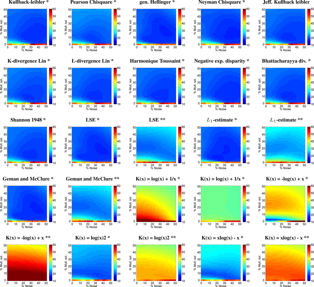
Figure 1.
Normalised RMSE (NRMSE) matrices for LCC retrieval using cost function displaying the impact of % noise (X-axis) against multiple solutions (Y-axis) in LUT-based RTM inversion. * : normalized; ** : non-normalized. The more bluish, the lower relative errors and thus the better the inversion.
Table 3.
Statistics (r2, RMSE, NRMSE) based on best evaluated NRMSE and corresponding mean multiple solutions (%) and noise level (%) for LCC retrieval. *: normalized; **: non-normalized. The “0.0 NRMSE” column represents the results without regularization options (left-bottom corner in matrices). Best inversion strategy is in bold font.
Moreover, these error matrices reveal the true interactions between the different cost functions and the regularization options. The matrices suggest that each of the tested CFs respond differently to the regularization options. It is interesting to see that in the majority of them a pattern with optimized performances appear (darkest blue), though the location and shape of this pattern may vary per CF. Thereby, not only CFs that are mathematically more alike led to similar trends, but also similarities appeared within the same CF family. This is particularly noticeable for the family of information measures, which shows robust LCC estimates across the whole noise and multiple solutions range, but also M-estimates CFs show similar behavior.
Interestingly, the matrices also revealed that data normalization governs the success of M-estimates. Excellent performances were achieved for the three M-estimates (LSE, L1-estimate, Geman and McClure), with best performances for L1-estimate (NRMSE of 17.6% at 6% multi solutions and 18% noise). Note that L1-estimate is proven to be optimal when distribution of errors have Laplace distribution. Also Neyman Chi-square and Generalized Hellinger reached such degree of accuracy (see Table 3). However, M-estimates performed considerably poorer (best results around 20%) when data is non-normalized, and matrices show that retrieval results are more affected by the two regularization options. Finally, the Minimum Contrast Estimation family yielded more irregular patterns. While in general they benefited from normalizing the dataset, only the “K(x) = log(x)2” and “K(x) = xlog(x) − x” proved to be robust CFs for LCC retrieval. In the absence of normalization best performances of these CFs were obtained at a maximal of tested noise level (i.e., 50%). Because these noise levels led to a considerable degradation of the simulated spectra it seems that these CFs only function well for LCC when data is normalized.
3.1.2. Leaf Area Index (LAI) Retrieval
Introducing noise and mean of multiple solutions considerably improved the LAI accuracies (Figure 2). Overall, on average relative errors almost halved: NRMSE from μ 42% to μ 22% (Table 4). However, in contrast to LCC retrievals, the information measures and the normalized M-estimates were no longer able to deliver good inversion results. In fact for the majority of CFs, normalization of the data caused that best results were achieved with the maximal degree of injected noise (i.e., 50%). Since such a spurious high noise level led to a considerable degradation of the simulated spectra it makes us concluding that normalization is not recommended for LAI retrieval. Consequently non-normalized M-estimates greatly improved accuracy of LAI retrievals. Particularly the classical LSE demonstrated to be the best CF (NRMSE: 15.3% at multiple solutions of 2% and noise of 14%), closely followed by the other M-estimates (L1-estimate, Geman and McClure). This means that in our example the errors tend to be Gaussian and solution is stable. Also these results suggest that controlling the normalization option can play an important role in LUT-based inversion. The contrast functions family did not perform very well and only normalized K(x) = log(x) + 1/x is able to retrieve LAI with best relative error of 16.5%. In comparison with LCC (Table 3) it can be noted that best LAI retrieval is performing slightly better (e.g., see NRMSE). Though, most important is to realize that different optimized inversion strategies were identified for both parameters. Finally, although not shown here for the sake of brevity, the retrieval capability of canopy-integrated chlorophyll content (CCC: LAI × LCC) was evaluated. CCC showed analogous patterns as LAI which suggests that this parameter, more than LCC, is the driving parameter of CCC. This can be probably attributed to the fact that LAI influences the whole spectral range, while LCC sensitive spectral range is limited to the beginning of the red edge.
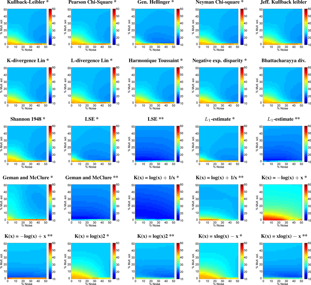
Figure 2.
NRMSE matrices for LAI retrieval using cost function displaying the impact of % noise (X-axis) against multiple solutions (Y-axis) in LUT-based RTM inversion. * : normalized; ** : non-normalized. The more bluish, the lower relative errors and thus the better the inversion.
Table 4.
Statistics (r2, RMSE, NRMSE) based on best evaluated NRMSE and corresponding mean multiple solutions (%) and noise level (%) for LAI retrieval. *: normalized; **: non-normalized. The ‘0.0 NRMSE’ column represents the results without regularization options (left-bottom corner in matrices). Best inversion result is in bold font.
3.2. Biophysical Parameters Mapping
Obtained systematic overview of the various inversion performances shows that deriving simultaneously multiple biophysical parameters using one inversion strategy is not the best choice. When parameters are correlated in a non-linear way it appears that the optimal cost functions are different for each parameter [36]. Hence, when we try to quantify LCC and LAI simultaneously will at least for one parameter lead to suboptimal performances. While in an operational setting it may be desirable to seek for an inversion strategy that leads to a balanced performance in the generation of all retrievable parameters [37], because of their non-linear dependency applying different retrieval strategies to different parameters is generally preferable. That is also the approach pursued here; for each parameter the best performing inversion strategy was applied (i.e., bolded in Tables 3 and 4). For LCC we applied L1-estimate (with mult. sol.: 4%, noise: 18%) and for LAI non-normalized normal distribution LSE (with mult. sol.: 2%, noise: 14%). Since in each of these strategies the mean of multiple solutions is applied it leads to the mapping of the mean estimates (μ) and associated standard deviation (±σ) (Figure 3).
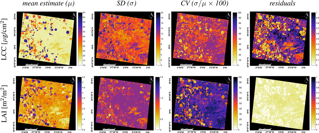
These maps are briefly interpreted. Starting with the μ-estimate maps, it can be observed that not only the irrigated circular fields with green biomass are clearly marked, but also pronounced within-field variations are notable by both parameters. These irrigated fields are characterized by a LCC above 40 μg/cm2 and LAI above 3. Areas with low LCC (≤25 μg/cm2) and LAI (≤1.5) are mainly bare soils, non-irrigated fallow lands or senescent or harvested cereal fields (wheat, barley). Particularly detailed spatial variation was encountered in the LAI map which suggests that greater sensitivity for this structural parameter is achieved. The ±σ-maps can be interpreted as uncertainty of the μ-estimate. The smaller the ±σ for a pixel, the lower that variation in multiple solutions is encountered during the inversion. Note that such ±σ map is also obtained by the MODIS LAI LUT-based retrieval method [20] and serves as a measure of the solution accuracy; starting from Collection 5, the ±σ (LAI) has been provided in the standard products. Here, at a glance, large uncertainty ranges arise when medium to high LCC conditions prevail. Similar studies observed the same large uncertainty ranges over dense canopies and are attributed to the saturation effect in the radiative transfer and the limited information provided in the a generation of the LUT [54–56]. However, since the ±σ also directly depends on the magnitude of μ, it may be more of interest to map the relative uncertainties, i.e., the coefficient of variation (CV; σ/μ). A relative indicator is of interest as it provides more information about the inversion process, i.e., a lower CV means a greater uniformity across the % best solutions, but it also allows a comparison of the inversion performance across all maps (Figure 3). For both LCC and LAI the CV maps suggest that the inversion process had least difficulty with the vegetated areas (circular irrigated fields), while most uncertainty was propagated over the fallow land and calcareous bare soils (South-East of image).
At the same time, parameter-independent information regarding the performance of the inversion process can also be obtained by mapping the residuals of the CFs. They provide another indicator on the inversion certainty. For each pixel, it indicates the degree of mismatch between the observed spectrum and the best matching simulated spectra. More than CV, these maps delineate the surfaces where the simulated spectra closely matched the observed spectra and thus a higher probability achieving a successful inversion. The maps suggest that particularly LAI was retrieved without difficulty, with perfect match over the vegetated areas. The inversion process had in all generality more difficulty with LCC, but large differences can be observed, leading to essentially the same earlier observed pattern; a close agreement over vegetated areas as opposed to senescent and non-vegetated lands. On the whole, the uncertainty analysis suggests that the inversion would benefit from a wider LUT with more spectral variation of senescent vegetation and bare soil surfaces.
4. Discussion
The upcoming S2 missions open opportunities to implement novel retrieval algorithms in operational processing chains. Specifically, there is a need for retrieval methods that are accurate, robust, and make fully use of the new S2 MSI bands. While in related works vegetation indices (e.g., [57,58]), or machine learning regression algorithms (e.g., [59,60]) have been proposed for S2 biophysical parameter retrieval, alternatively we advocate the method of LUT-based RTM inversion. Although this approach is not new, it has never been exploited to the fullest. Here we systematically analyzed the impact of CFs and regularization options. It led to consolidated findings discussed below.
4.1. Cost Functions and Regularization Options
To mitigate the drawback of ill-posedness instead of introducing prior information it was opted to exploit the performances of alternative CFs in combination with regularization options. The rationale for evaluating CFs as opposed to the widely used LSE (or RMSE) is that propagated uncertainties and errors, e.g., due to uncertainties in instrument calibration, variations in atmospheric composition or simplifying assumptions in the representation of canopy and soil background, distort the residuals and in many cases violate a key assumption for using LSE, which corresponds to the maximum likelihood estimation with Gaussian distribution of residuals [36]. Nevertheless in our presented dataset it was found that LSE outperformed most of the alternative tested CFs for LCC with the condition of data normalization. Only the “L1-estimate” function performed slightly better, which suggest that the errors rather tend to be distributed according to a Laplace distribution. Moreover normalization led to better performances with respect of varying added noise and multiple solutions in the inversion. Hence, data normalization provides good accuracy for LCC inversion and can be explained as follows. Variation in reflectance as a function of chlorophyll absorption occurs predominantly in the visible part of the spectrum and declines rapidly once entering red edge [61], i.e., encompassing S2 bands B2 to B5. Accordingly, in PROSPECT the chlorophyll absorption coefficients start to become negligible from 730 nm onwards. A closer look to the simulated dataset revealed that normalization compresses the dataset and so ensures that the observation spectrum falls within the same range. This particularly plays a role in the visible part of the spectrum. As reflectance of vegetated surfaces in the visible is typically low (often ≤10%) and variation in this region is narrow, normalization helps reaching a better match in this region between simulated and observed spectra. Conversely, data normalization did not lead to the good CFs performance for LAI, and non-normalized data in combination with multiple solutions and the CF LSE showed to be the most successful. It should herewith be noted that LAI variation (i.e., vegetation density) causes a spectral variation over the whole VNIR spectrum, i.e., S2 bands from B2 to B8. Thereby, the larger magnitude of reflectance in the NIR and greater LAI-induced variation in comparison to the visible part makes NIR an important region for LAI retrieval in LUT-based inversion. Consequently, a spectral observation easily falls within such a broad range of simulated spectral variation, and compression of the simulations through normalization tend to disturb the matching between observed and simulated spectra. A standard inversion scheme proved thus to be most successful for LAI retrieval. Effectively, many publications demonstrated that LAI can be relatively easily retrieved without data normalization (e.g., [19,23,38,62]). We are not aware of other studies that have systematically evaluated the role of data normalization in LUT-based inversion, though proper usage may greatly improve accuracies. For instance, it explains why in [37] RMSE was performing poorly for LAI where this CF was employed in normalized mode only. It may also explain why similar studies reported a poor LCC inversion as there no mentioning of normalizing the data has been made [19,62]. Further, as earlier observed in [37], this study confirms for 18 tested CFs that introducing some degree of noise and mean of multiple solutions in the inversion can lead to improved inversion performances, though its actual impact strongly depended on the considered parameter and cost function. Hence developing optimized inversion strategies for each single retrievable parameter is strongly recommended.
4.2. Inversion Performance
The evaluation of various CFs and regularization options led to identified inversion strategies with accuracies of r2 on the order of 0.73–0.81 and relative errors (NRMSE) of 15%–18%. A range of 15%–20% is regarded as the currently achievable accuracy for LAI from EO data [63]. However, a retrieval accuracy of 10% is targeted for the S2 mission [64]. It should thereby be emphasized that the validation dataset consisted of all kinds of crop types, including row crops such as maize, potatoes, onions and vineyards. In related work by [19,23] this degree of accuracy was only achieved over single crops, and it was concluded that PROSAIL fails to invert over multi-species canopies. Thereby, various types of uncertainties have been identified that may lead to suboptimal retrievals, with respect to model usage (e.g., 1D vs. 3D models), parametrization and validation data [22]. Suggestions for improvements typically refer to adding more prior information at the level of individual parcels, i.e., through a more specialized LUT (e.g., [20,22,23,51,65,66]). While such strategies could be beneficial for dedicated sites, site-specific information is usually unavailable in an operational context for larger areas. The proposed regularization options yielded robust inversion schemes that are easily applicable over full scenes covering heterogeneous canopy surfaces. Although most of the CFs within the same family perform alike and are in principle thus replaceable, performance gain is especially reached in combination with applying multiple solutions and noise in the inversion. Moreover, further improvements can be achieved by applying CFs that require tuning of additional parameters. In general tuning parameters in CFs would lead to refined inversion strategies as compared to standalone CFs (e.g., see [36,37]). Further research is planned to have these tunable CFs optimized in an automated fashion.
At the same time, information about the inversion uncertainty on a pixel-by-pixel basis may be as relevant as overall accuracies calculated from a limited set of ground-based validation data. Uncertainty indicators were obtained through mapping of CV and residuals. The CV is an indicator of the uncertainty range around the mean estimate, which tells something about the ill-posedness of the inversion of a retrievable parameter, whereas the residuals tells us how much the observed spectra deviate against that from the LUT spectra in the inversion scheme. These quality layers allow masking out uncertain estimates.
Both indicators showed a consistent spatial trend for all parameters: pixels of vegetated surfaces matched closely with the synthetic reflectance database while pixels of non-vegetated surfaces faced more difficulties. Two reasons can be identified for this discrepancy: (1) the inversion strategy was optimized against validation data that was exclusively collected on vegetated areas; and (2) PROSAIL is a canopy reflectance model and thus well able to detect variation in vegetation properties. Hence the generated LUT and final inversion scheme were not optimized to detect variations in dried-out fallow and bare soil lands. For retrievals over full images there is thus a need for regulating the inversion strategy both over vegetated targets as well over non-vegetated targets. Therefore, while having inversion over vegetated canopies resolved, adequately processing non-vegetated surfaces remains to be optimized. To start with, further efforts are needed in the generation and evaluation of more generic LUTs, i.e., including spectra of kinds of soil types, man-made surfaces and water bodies. PROSAIL alone is not able to deliver this; hence coupling with a generic soil reflectance model that enables generating a variety of non-vegetated reflectances would be a next step to do. It should hereby also be noted that the 20 m-S2 bands B11 and B12 have not been considered in this study because of falling outside the CHRIS range. These bands in the SWIR are known to be sensitive to vegetation structure [67] and can better distinguish between dried-out fallow and non-vegetated lands. It is expected that inclusion of the SWIR bands will further improve the retrieval quality. Another promising avenue to be investigated is relying on vegetation indices to spatially constrain the LUTs. For instance, vegetation indices are able to detect bare soil, water bodies, sparsely vegetated areas and densely vegetated areas (e.g., see also [32]). That information could then be used to constrain LUTs on a per-pixel basis and is currently explored to be implemented into ARTMO.
5. Conclusions
LUT-based inversion is considered as a physically-sound retrieval method to quantify biophysical parameters from Earth observation imagery, but the full potential of this method has not been consolidated yet. Here, we have systematically compared 18 different cost functions (CFs) originating from three major statistical families: information measures, M-estimates and minimum contrast methods. All these CFs are standalone functions that can be directly implemented in processing algorithms. These CFs were fully exploited through various regularization options, i.e., adding noise, multiple solutions and normalization, for the benefit of improved LCC and LAI estimations. Inversion of the PROSAIL model against a simulated 20 m Sentinel-2 imagery (8 bands: B2-B8a) over an agricultural site (Barrax, Spain) and against a validation dataset led to the following conclusions:
- All evaluated CFs and biophysical parameters gained from regularization options such as adding some noise and multiple solutions in the inversion. These options with proper adjustment can significantly reduce relative errors.
- With introduction of multiple solutions and noise information measures CFs proved to be successful for deriving LCC. However best LCC results were achieved with the M-estimate L1 (NRMSE of 17.6% at 6% multiple solutions and 18% noise) when data is normalized.
- Data normalization appeared to be unsuccessful for retrieving LAI. Here, the classical LSE yielded best results for non-normalized data; NRMSE of 15.3% at 6% multiple solutions and 18% noise, and 16.4% at 16% multiple solutions and 0% noise, respectively.
Systematic analysis for each biophysical parameter identified different optimized inversion strategy, which was subsequently applied to pixel-by-pixel Sentinel-2 imagery. It provided us with maps of mean estimates and associated statistics and showed insight into the uncertainty of the retrievals (e.g., coefficient of variation and residuals). These indicators showed that inversions were most successful over densely vegetated areas. PROSAIL had more difficulty with processing fallow and non-vegetated lands, but that is expected to be resolved with an adjusted LUT and the addition of SWIR bands in actual Sentinel-2 data.
The bottom line of this work is that, despite common practice, no single inversion strategy was found to be optimal for deriving multiple biophysical parameters. While some general trends with respect to regularization options and CFs was revealed, it is the data distribution that determines the success of the inversion strategy, which is governed by the biophysical parameter, the generated LUT, the spectral bands and the validation data. It is therefore recommended to test different CFs and regularization options before implementing an inversion scheme in a processing chain.
Acknowledgments
This paper has been partially supported by the Spanish Ministry for Science and Innovation under projects: AYA2010-21432-C02-01 and CSD2007-00018. Three anonymous reviewers are thanked for providing comments that helped with improving the quality of the original manuscript.
Conflict of Interest
The authors declare no conflict of interest.
References
- Whittaker, R.H.; Marks, P.L. Methods of Assessing Terrestrial Productivity. In Primary Productivity of the Biosphere; Springer Verlag: Berlin/Heidelberg, Germany, 1975; pp. 55–118. [Google Scholar]
- Lichtenthaler, H.K. Chlorophylls and carotenoids: Pigments of photosynthetic biomembranes. Methods Enzymol 1987, 148, 350–382. [Google Scholar]
- Malenovský, Z.; Rott, H.; Cihlar, J.; Schaepman, M.; García-Santos, G.; Fernandes, R.; Berger, M. Sentinels for science: Potential of Sentinel-1, -2, and -3 missions for scientific observations of ocean, cryosphere, and land. Remote Sens. Environ 2012, 120, 91–101. [Google Scholar]
- Lichtenthaler, H.K.; Lang, M.; Sowinska, M.; Heisel, F.; Miehe, J.A. Detection of vegetation stress via a new high resolution fluorescence imaging system. J. Plant Physiol 1996, 148, 599–612. [Google Scholar]
- Sampson, P.H.; Zarco-Tejada, P.J.; Mohammed, G.H.; Miller, J.R.; Noland, T.L. Hyperspectral remote sensing of forest condition: Estimating chlorophyll content in tolerant hardwoods. For. Sci 2003, 49, 381–391. [Google Scholar]
- Dorigo, W.A.; Zurita-Milla, R.; de Wit, A.J.W.; Brazile, J.; Singh, R.; Schaepman, M.E. A review on reflective remote sensing and data assimilation techniques for enhanced agroecosystem modeling. Int. J. Appl. Earth Obs. Geoinf 2007, 9, 165–193. [Google Scholar]
- Delegido, J.; Verrelst, J.; Meza, C.; Rivera, J.; Alonso, L.; Moreno, J. A red-edge spectral index for remote sensing estimation of green LAI over agroecosystems. Eur. J. Agron 2013, 46, 42–52. [Google Scholar]
- Gianquinto, G.; Orsini, F.; Fecondini, M.; Mezzetti, M.; Sambo, P.; Bona, S. A methodological approach for defining spectral indices for assessing tomato nitrogen status and yield. Eur. J. Agron 2011, 35, 135–143. [Google Scholar]
- Baret, F.; Hagolle, O.; Geiger, B.; Bicheron, P.; Miras, B.; Huc, M.; Berthelot, B.; Niço, F.; Weiss, M.; Samain, O.; et al. LAI, fAPAR and fCover CYCLOPES global products derived from VEGETATION. Part 1: Principles of the algorithm. Remote Sens. Environ 2007, 110, 275–286. [Google Scholar]
- Myneni, R.; Hoffman, S.; Knyazikhin, Y.; Privette, J.; Glassy, J.; Tian, Y.; Wang, Y.; Song, X.; Zhang, Y.; Smith, G.; et al. Global products of vegetation leaf area and fraction absorbed PAR from year one of MODIS data. Remote Sens. Environ 2002, 83, 214–231. [Google Scholar]
- Ganguly, S.; Nemani, R.; Zhang, G.; Hashimoto, H.; Milesi, C.; Michaelis, A.; Wang, W.; Votava, P.; Samanta, A.; Melton, F.; et al. Generating global leaf area index from landsat: Algorithm formulation and demonstration. Remote Sens. Environ 2012, 122, 185–202. [Google Scholar]
- Dash, J.; Curran, P. The MERIS terrestrial chlorophyll index. Int. J. Remote Sens 2004, 25, 5403–5413. [Google Scholar]
- Bacour, C.; Baret, F.; Béal, D.; Weiss, M.; Pavageau, K. Neural network estimation of LAI, fAPAR, fCover and LAI × Cab, from top of canopy MERIS reflectance data: Principles and validation. Remote Sens. Environ 2006, 105, 313–325. [Google Scholar]
- Houborg, R.; Boegh, E. Mapping leaf chlorophyll and leaf area index using inverse and forward canopy reflectance modeling and SPOT reflectance data. Remote Sens. Environ 2008, 112, 186–202. [Google Scholar]
- Houborg, R.; Anderson, M.; Daughtry, C. Utility of an image-based canopy reflectance modeling tool for remote estimation of LAI and leaf chlorophyll content at the field scale. Remote Sens. Environ 2009, 113, 259–274. [Google Scholar]
- Stuffler, T.; Kaufmann, C.; Hofer, S.; Förster, K.; Schreier, G.; Mueller, A.; Eckardt, A.; Bach, H.; Penné, B.; Benz, U.; et al. The EnMAP hyperspectral imager-An advanced optical payload for future applications in Earth observation programmes. Acta Astronaut 2007, 61, 115–120. [Google Scholar]
- Labate, D.; Ceccherini, M.; Cisbani, A.; De Cosmo, V.; Galeazzi, C.; Giunti, L.; Melozzi, M.; Pieraccini, S.; Stagi, M. The PRISMA payload optomechanical design, a high performance instrument for a new hyperspectral mission. Acta Astronaut 2009, 65, 1429–1436. [Google Scholar]
- Roberts, D.; Quattrochi, D.; Hulley, G.; Hook, S.; Green, R. Synergies between VSWIR and TIR data for the urban environment: An evaluation of the potential for the Hyperspectral Infrared Imager (HyspIRI) decadal survey mission. Remote Sens. Environ 2012, 117, 83–101. [Google Scholar]
- Darvishzadeh, R.; Skidmore, A.; Schlerf, M.; Atzberger, C. Inversion of a radiative transfer model for estimating vegetation LAI and chlorophyll in a heterogeneous grassland. Remote Sens. Environ 2008, 112, 2592–2604. [Google Scholar]
- Knyazikhin, Y.; Kranigk, J.; Myneni, R.; Panfyorov, O.; Gravenhorst, G. Influence of small-scale structure on radiative transfer and photosynthesis in vegetation canopies. J. Geophys. Res. D 1998, 103, 6133–6144. [Google Scholar]
- Durbha, S.; King, R.; Younan, N. Support vector machines regression for retrieval of leaf area index from multiangle imaging spectroradiometer. Remote Sens. Environ 2007, 107, 348–361. [Google Scholar]
- Combal, B.; Baret, F.; Weiss, M.; Trubuil, A.; Mace, D.; Pragnère, A.; Myneni, R.; Knyazikhin, Y.; Wang, L. Retrieval of canopy biophysical variables from bidirectional reflectance using prior information to solve the ill-posed inverse problem. Remote Sens. Environ 2003, 84, 1–15. [Google Scholar]
- Richter, K.; Atzberger, C.; Vuolo, F.; Weihs, P.; D’Urso, G. Experimental assessment of the Sentinel-2 band setting for RTM-based LAI retrieval of sugar beet and maize. Can. J. Remote Sens 2009, 35, 230–247. [Google Scholar]
- Weiss, M.; Baret, F.; Myneni, R.; Pragnère, A.; Knyazikhin, Y. Investigation of a model inversion technique to estimate canopy biophysical variables from spectral and directional reflectance data. Agronomie 2000, 20, 3–22. [Google Scholar]
- Fang, H.; Liang, S. A hybrid inversion method for mapping leaf area index from MODIS data: Experiments and application to broadleaf and needleleaf canopies. Remote Sens. Environ 2005, 94, 405–424. [Google Scholar]
- Qu, Y.; Wang, J.; Wan, H.; Li, X.; Zhou, G. A Bayesian network algorithm for retrieving the characterization of land surface vegetation. Remote Sens. Environ 2008, 112, 613–622. [Google Scholar]
- Walthall, C.; Dulaney, W.; Anderson, M.; Norman, J.; Fang, H.; Liang, S. A comparison of empirical and neural network approaches for estimating corn and soybean leaf area index from Landsat ETM+ imagery. Remote Sens. Environ 2004, 92, 465–474. [Google Scholar]
- Weiss, M.; Baret, F. Evaluation of canopy biophysical variable retrieval performances from the accumulation of large swath satellite data. Remote Sens. Environ 1999, 70, 293–306. [Google Scholar]
- Jacquemoud, S.; Baret, F.; Andrieu, B.; Danson, F.; Jaggard, K. Extraction of vegetation biophysical parameters by inversion of the PROSPECT+SAIL models on sugar beet canopy reflectance data. Application to TM and AVIRIS sensors. Remote Sens. Environ 1995, 52, 163–172. [Google Scholar]
- Baret, F.; Buis, S. Estimating Canopy Characteristics from Remote Sensing Observations. Review of Methods and Associated Problems. In Advances in Land Remote Sensing: System, Modeling, Inversion and Application; Liang, S., Ed.; Springer: Berlin, Germany, 2008; pp. 173–201. [Google Scholar]
- Combal, B.; Baret, F.; Weiss, M. Improving canopy variables estimation from remote sensing data by exploiting ancillary information. Case study on sugar beet canopies. Agronomie 2002, 22, 205–215. [Google Scholar]
- Dorigo, W.; Richter, R.; Baret, F.; Bamler, R.; Wagner, W. Enhanced automated canopy characterization from hyperspectral data by a novel two step radiative transfer model inversion approach. Remote Sens 2009, 1, 1139–1170. [Google Scholar]
- Koetz, B.; Baret, F.; Poilvé, H.; Hill, J. Use of coupled canopy structure dynamic and radiative transfer models to estimate biophysical canopy characteristics. Remote Sens. Environ 2005, 95, 115–124. [Google Scholar]
- Richter, K.; Atzberger, C.; Vuolo, F.; D’Urso, G. Evaluation of Sentinel-2 spectral sampling for radiative transfer model based LAI estimation of wheat, sugar beet, and maize. IEEE J. Sel. Top. Appl. Earth Obs. Remote Sens 2011, 4, 458–464. [Google Scholar]
- Darvishzadeh, R.; Matkan, A.A.; Dashti Ahangar, A. Inversion of a radiative transfer model for estimation of rice canopy chlorophyll content using a lookup-table approach. IEEE J. Sel. Top. Appl. Earth Obs. Remote Sens. 2012, PP, 1–9. [Google Scholar]
- Leonenko, G.; North, P.; Los, S. Statistical distances and their applications to biophysical parameter estimation: Information measures, M-estimates, and minimum contrast methods. Remote Sens 2013, 5, 1355–1388. [Google Scholar]
- Verrelst, J.; Rivera, J.; Leonenko, G.; Moreno, J. Optimizing LUT-based RTM inversion for semiautomatic mapping of crop biophysical parameters from Sentinel-2 and -3 data: Role of cost functions. IEEE Trans. Geosci. Remote Sens. 2013, in press.. [Google Scholar]
- Atzberger, C.; Richter, K. Spatially constrained inversion of radiative transfer models for improved LAI mapping from future Sentinel-2 imagery. Remote Sens. Environ 2012, 120, 208–218. [Google Scholar]
- Chen, J.; Pavlic, G.; Brown, L.; Cihlar, J.; Leblanc, S.; White, H.; Hall, R.; Peddle, D.; King, D.; Trofymow, J.; et al. Derivation and validation of Canada-wide coarse-resolution leaf area index maps using high-resolution satellite imagery and ground measurements. Remote Sens. Environ 2002, 80, 165–184. [Google Scholar]
- Kullback, S.; Leibler, R. On information and sufficiency. Ann. Math. Stat 1951, 22, 79–86. [Google Scholar]
- Pardo, L. Statistical Inference Based on Divergence Measures, Statistics: A Series Textbooks and Monographs; Chapman and Hall/CRC: Boca Raton, FL, USA, 2006. [Google Scholar]
- Staudte, R.; Sheather, S. Robust Estimation and Testing; Wiley: New York, NY, USA, 1990. [Google Scholar]
- Taniguchi, M. On estimation of parameters of Gaussian stationary processes. J. Appl. Probab 1979, 16, 575–591. [Google Scholar]
- Gandía, S.; Fernández, G.; Garcia, J.C.; Moreno, J. Retrieval of Vegetation Biophysical Variables from CHRIS/PROBA Data in the SPARC Campaign. Proceedings of the 2nd CHRIS/PROBAWorkshop, Frascati, Italy, 28–30 April 2004.
- Fernández, G.; Moreno, J.; Gandía, S.; Martínez, B.; Vuolo, F.; Morales, F. Statistical Variability of Field Measurements of Biophysical Parameters in SPARC-2003 and SPARC-2004 Campaigns. Proceedings of the SPARC Workshop WPP-250, Enschede, The Netherlands, 4–5 July 2005.
- Drusch, M.; Del Bello, U.; Carlier, S.; Colin, O.; Fernandez, V.; Gascon, F.; Hoersch, B.; Isola, C.; Laberinti, P.; Martimort, P.; et al. Sentinel-2: ESA’s optical high-resolution mission for GMES operational services. Remote Sens. Environ 2012, 120, 25–36. [Google Scholar]
- Barnsley, M.J.; Settle, J.J.; Cutter, M.A.; Lobb, D.R.; Teston, F. The PROBA/CHRIS mission: A low-cost smallsat for hyperspectral multiangle observations of the earth surface and atmosphere. IEEE Trans. Geosci. Remote Sens 2004, 42, 1512–1520. [Google Scholar]
- Alonso, L.; Moreno, J. Advances and Limitations in A Parametric Geometric Correction of CHRIS/PROBA Data. Proceedings of the 3rd CHRIS/Proba Workshop, Frascati, Italy, 21–23 March 2005.
- Guanter, L.; Alonso, L.; Moreno, J. A method for the surface reflectance retrieval from PROBA/CHRIS data over land: Application to ESA SPARC campaigns. IEEE Trans. Geosci. Remote Sens 2005, 43, 2908–2917. [Google Scholar]
- Verrelst, J.; Rivera, J.; Alonso, L.; Moreno, J. ARTMO: An Automated Radiative Transfer Models Operator Toolbox for Automated Retrieval of Biophysical Parameters through Model Inversion. Proceedings of EARSeL 7th SIG-Imaging Spectroscopy Workshop, Edinburgh, UK, 11–13 April 2011.
- Verrelst, J.; Romijn, E.; Kooistra, L. Mapping vegetation density in a heterogeneous river floodplain ecosystem using pointable CHRIS/PROBA data. Remote Sens 2012, 4, 2866–2889. [Google Scholar]
- Jacquemoud, S.; Verhoef, W.; Baret, F.; Bacour, C.; Zarco-Tejada, P.; Asner, G.; François, C.; Ustin, S. PROSPECT + SAIL models: A review of use for vegetation characterization. Remote Sens. Environ 2009, 113, S56–S66. [Google Scholar]
- Feret, J.B.; François, C.; Asner, G.P.; Gitelson, A.A.; Martin, R.E.; Bidel, L.P.R.; Ustin, S.L.; le Maire, G.; Jacquemoud, S. PROSPECT-4 and 5: Advances in the leaf optical properties model separating photosynthetic pigments. Remote Sens. Environ 2008, 112, 3030–3043. [Google Scholar]
- Garrigues, S.; Lacaze, R.; Baret, F.; Morisette, J.; Weiss, M.; Nickeson, J.; Fernandes, R.; Plummer, S.; Shabanov, N.; Myneni, R.; et al. Validation and intercomparison of global leaf area index products derived from remote sensing data. J. Geophys. Res.-Biogeosci. 2008, 113. [Google Scholar] [CrossRef]
- Pinty, B.; Lavergne, T.; Vobbeck, M.; Kaminski, T.; Aussedat, O.; Giering, R.; Gobron, N.; Taberner, M.; Verstraete, M.; Widlowski, J.L. Retrieving surface parameters for climate models from Moderate Resolution Imaging Spectroradiometer (MODIS)-Multiangle Imaging Spectroradiometer (MISR) albedo products. J. Geophy. Res.-Atmos. 2007, 112. [Google Scholar] [CrossRef]
- Weiss, M.; Baret, F.; Garrigues, S.; Lacaze, R. LAI and fAPAR CYCLOPES global products derived from VEGETATION. Part 2: validation and comparison with MODIS collection 4 products. Remote Sens. Environ 2007, 110, 317–331. [Google Scholar]
- Clevers, J.; Gitelson, A. Remote estimation of crop and grass chlorophyll and nitrogen content using red-edge bands on Sentinel-2 and -3. ITC J. 2013; in press. [Google Scholar]
- Delegido, J.; Verrelst, J.; Alonso, L.; Moreno, J. Evaluation of sentinel-2 red-edge bands for empirical estimation of green LAI and chlorophyll content. Sensors 2011, 11, 7063–7081. [Google Scholar]
- Verrelst, J.; Muñoz, J.; Alonso, L.; Delegido, J.; Rivera, J.; Camps-Valls, G.; Moreno, J. Machine learning regression algorithms for biophysical parameter retrieval: Opportunities for Sentinel-2 and -3. Remote Sens. Environ 2012, 118, 127–139. [Google Scholar]
- Richter, K.; Hank, T.; Vuolo, F.; Mauser, W.; D’Urso, G. Optimal exploitation of the Sentinel-2 spectral capabilities for crop leaf area index mapping. Remote Sens 2012, 4, 561–582. [Google Scholar]
- Gitelson, A.; Merzlyak, M.; Lichtenthaler, H. Detection of red edge position and chlorophyll content by reflectance measurements near 700 nm. J. Plant Physiol 1996, 148, 501–508. [Google Scholar]
- Si, Y.; Schlerf, M.; Zurita-Milla, R.; Skidmore, A.; Wang, T. Mapping spatio-temporal variation of grassland quantity and quality using MERIS data and the PROSAIL model. Remote Sens. Environ 2012, 121, 415–425. [Google Scholar]
- Baret, F. Biophysical vegetation variables retrieval from remote sensing observations. Proc. SPIE 2010, 7824, 17–19. [Google Scholar]
- Drusch, M.; Gascon, F.; Berger, M. Sentinel-2 Mission Requirements Document, 2010. Available online: http://esamultimedia.esa.int/docs/GMES/Sentinel-2_MRD.pdf (accessed on 27 April 2013).
- Atzberger, C. Object-based retrieval of biophysical canopy variables using artificial neural nets and radiative transfer models. Remote Sens. Environ 2004, 93, 53–67. [Google Scholar]
- Meroni, M.; Colombo, R.; Panigada, C. Inversion of a radiative transfer model with hyperspectral observations for LAI mapping in poplar plantations. Remote Sens. Environ 2004, 92, 195–206. [Google Scholar]
- Brown, L.; Chen, J.; Leblanc, S.; Cihlar, J. A shortwave infrared modification to the simple ratio for LAI retrieval in boreal forests: An image and model analysis. Remote Sens. Environ 2000, 71, 16–25. [Google Scholar]
© 2013 by the authors; licensee MDPI, Basel, Switzerland This article is an open access article distributed under the terms and conditions of the Creative Commons Attribution license (http://creativecommons.org/licenses/by/3.0/).