Estimating Composite Curve Number Using an Improved SCS-CN Method with Remotely Sensed Variables in Guangzhou, China


Abstract
: The rainfall and runoff relationship becomes an intriguing issue as urbanization continues to evolve worldwide. In this paper, we developed a simulation model based on the soil conservation service curve number (SCS-CN) method to analyze the rainfall-runoff relationship in Guangzhou, a rapid growing metropolitan area in southern China. The SCS-CN method was initially developed by the Natural Resources Conservation Service (NRCS) of the United States Department of Agriculture (USDA), and is one of the most enduring methods for estimating direct runoff volume in ungauged catchments. In this model, the curve number (CN) is a key variable which is usually obtained by the look-up table of TR-55. Due to the limitations of TR-55 in characterizing complex urban environments and in classifying land use/cover types, the SCS-CN model cannot provide more detailed runoff information. Thus, this paper develops a method to calculate CN by using remote sensing variables, including vegetation, impervious surface, and soil (V-I-S). The specific objectives of this paper are: (1) To extract the V-I-S fraction images using Linear Spectral Mixture Analysis; (2) To obtain composite CN by incorporating vegetation types, soil types, and V-I-S fraction images; and (3) To simulate direct runoff under the scenarios with precipitation of 57mm (occurred once every five years by average) and 81mm (occurred once every ten years). Our experiment shows that the proposed method is easy to use and can derive composite CN effectively.1. Introduction
Surface runoff is an important hydrologic variable used widely in water resources studies. The rainfall-runoff process is a complex, dynamic and nonlinear process, which is affected by many, often interrelated, and physical factors. Reliable predictions of quantity and rate of runoff from land surface into streams and rivers are difficult and time-consuming to obtain for ungauged watersheds. As a result, many researchers have developed various methods to estimate both human influence on changes in surface runoff, especially storm runoff, and consequent effects on downstream activities. Many runoff simulations models, such as the Sacramento model [1], Tank model [2], HBV model [3], MIKE 11/NAM model [4,5] and Soil Conservation Service curve number (SCS-CN) method, have been proposed and applied to urban runoff prediction. Among these models, the SCS-CN is one of the most enduring methods for estimating the volume of direct surface runoff in ungauged rural catchments [6]. It is also noted that several complex models such as Soil and Water Assessment Tool (SWAT) [7], Hydrologic Modeling System (HEC-HMS), Erosion Productivity Impact Calculator (EPIC), and Agricultural Non-Point Source Pollution Model (AGNPS) have been developed based on SCS-CN method [8].
The SCS-CN method developed by Natural Resources Conservation Service (NRCS) of the United States Department of Agriculture (USDA) is widely used for predicting direct surface runoff volume for a given rainfall event and estimating the volumes and peak rates of surface runoff in rural catchments [6]. It forms the basic hydrological model incorporated into many USDA SCS systems such as CREAMS [9] and SPUR [10]. The SCS-CN model has a key parameter, Curve Number (CN), which is developed from an empirical study of runoff in small catchments and hill slope plots monitored by the NRCS of the USDA [8]. The CN method expresses runoff volume as a function of rainfall volume, hydrologic storage, and initial abstraction [11]. The CN value depends on land surface characteristics and hydro-soil conditions. The higher the CN value, the higher the volume of direct surface runoff. In general, CN can be found in the TR-55 look-up table [12], and is derived from several surface features. However, due to the complexity of land surface features in urban environments, the CN in the TR-55 cannot be applied to all surface types. Therefore, previous studies have attempted to improve CN calculation methods based on the TR-55. Many researchers developed CN calculation methods by incorporating land cover information and the original CN in TR-55. Hong and Adler (2008) developed a global SCS-CN runoff map using land cover, soils and antecedent moisture conditions [13]. Canters et al. (2006) calculated CN at the catchment level by combining impervious surface, vegetation, bare soil and water/shade information [14]. Joseph (2011) proposed CN can be calculated by integrating the percentages of impervious surface, tree canopy density and pervious surface [15]. Furthermore, CN may be calculated via the combination of water, dense forest, and sand [16]. Christianna (2009) discussed a composite CN calculation method by integrating vegetation, impervious surface and soil [17], and an average CN value of the whole catchment was also calculated. Apparently, most previous studies showed that impervious surface played an important role in computing the CN, because it affected the infiltration of the surface water. In addition, the number of land cover types described in TR-55 is so enormous that they are difficult to be classified from the medium resolution remote sensing imagery with proper accuracy [12].
Based on the considerations of urban landscape complexity and the characteristics of medium-resolution satellite imagery, this paper intends to develop a method to calculate the composite CN with the vegetation-impervious surface-soil (V-I-S) model [18], NDVI and soil types. First, soil types and NDVI are classified into several classes, respectively. Second, each class of soil type and NDVI are given an initial CNs (initial CN of soil) and CNv (initial CN of vegetation), respectively. Lastly, the CN is calculated by computing the percentages of impervious surface, NDVI class, and soil class. Impervious surface is the land surface through which water cannot infiltrate. Impervious anthropogenic features include roads, driveways, highways, sidewalks, parking lots and rooftops.
The percentage of impervious surface is a critical factor in the generation of surface runoff. Impervious surface proposed by Ridd (1995) may be viewed as a characteristic index of urbanization. Urban vegetation consists of a set of features that may include forest, bush, grass, orchard, and bare soil can usually be found in the construction sites in the urban areas. The fraction images of V-I-S can be extracted from various remote sensing images, including high spatial resolution images such as QuickBird and IKONOS [19,20], medium resolution images such as Landsat TM and Terra ASTER [19,21–24], and coarse resolution images such as DMSP-OLS and In-SAR data [25,26]. Many methods for extracting V-I-S have been developed in recent years. Linear spectral mixture analysis (LSMA) has been widely used to extract the fraction images of V-I-S [23,27].
The objectives of this paper are: (1) to extract the vegetation, impervious surface and soil fractions from remotely sensed imagery; (2) to develop a method of computing composite CN based on the V-I-S model; and (3) to simulate surface runoff volume in Guangzhou City under the scenarios of 57 and 81 mm (rainfall intensity: per hour) precipitation [28].
2. Data and Methodology
2.1. Study Area and Data
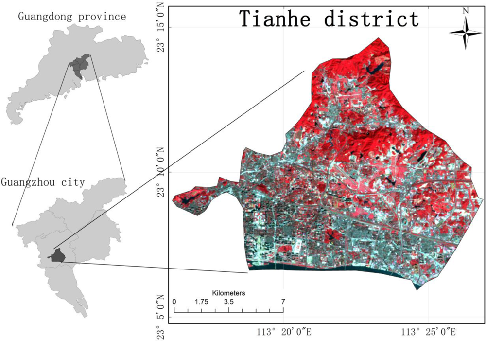
Guangzhou, the capital of the Guangdong province, is the political, economic, and cultural center of the Guangdong province and a transportation hub in southern China. Tianhe district (Figure 1) is a new Central Business District (CBD) of Guangzhou which covers 139 km2 with the population of 0.62 million in 2005. It is located in the north bank of Pearl River, east of Guangzhou city. It has a subtropical climate, which is strongly influenced by the Asian monsoon, with an average annual temperature between 21 °C and 23 °C, and an average precipitation from 1,600 to 2,600 mm.
A Landsat-5 TM image (Path 122/ Row44, acquired on 11 February 2009) is used for extracting the fraction images of V-I-S. The TM image is rectified to the Universal Transverse Mercator projection system. A geometric correction is performed to register the TM image to high resolution images (SPOT 2010) obtained from Google Earth and the RMSE (Root Mean Square Error) for geometric correction is 0.2928. In addition, radiometric correction is performed using the calibration parameter file (CPF) released by the Earth Resources Observation Systems Data Center, United States Geological Survey (USGS). Soil types are derived from the soil image of Guangdong Province with the scale of 1:1,000,000 [29]. The precipitation data of 11-02-2009 (including preceding five days data) are obtained from the Meteorological Bureau of Tianhe District. The high resolution SPOT images are used as ground reference to assess the accuracy of the spectral un-mixing result and the classification of NDVI. A total of 150 random samples are generated and the RMSE is calculated [22].
2.2. Extracting Vegetation, Impervious Surface and Soil Fractions
The composite CN is calculated based on the impervious surface which was derived from linear spectral mixture analysis (LSMA). LSMA is regarded as a physically based image processing technique that supports repeatable and accurate extraction of quantitative sub-pixel information [30–32]. It assumes that the spectrum measured by a sensor is a linear combination of the spectra of all components within the pixel [30,33]. The mathematical model of LSMA can be expressed as:
It is a key step to select proper end-members during the process of un-mixing the mixed pixels. Many approaches have been developed for selecting end-members such as measured spectrum based and image based methods. The image based end-member selection method is chosen and the Maximum Noise Fraction (MNF) is carried out to help select end-members. The MNF may integrate almost 90% of the original information on the first, second or third components and can minimize the influence of band-to-band correlation [34].
In the study, water is masked out using the normalized difference water index method [35]. Four end-members (high albedo, low albedo, vegetation and soil) are selected through the MNF images. The impervious surface fraction image is generated by adding the high albedo fraction image and the low albedo fraction image [36]. Root Mean Square Error (RMSE) is computed to evaluate the accuracy of the un-mixing results. The RMSE can be expressed as follows:
2.3. The SCS-CN Method
The general runoff equation is as follows:
The above equation shows that S is the only parameter that determines the volume of direct runoff. The retention parameter S is related to the value of CN by
CN can be found in the TR-55 table or can be calculated as the com posite CN [11]. The Equation (6) shows that the CN decreases as the potential maximum retention S increases. The equation shows the sensitivity of the change in water retention capacity to the CN range.
2.4. Improved Composite CN Computation Method
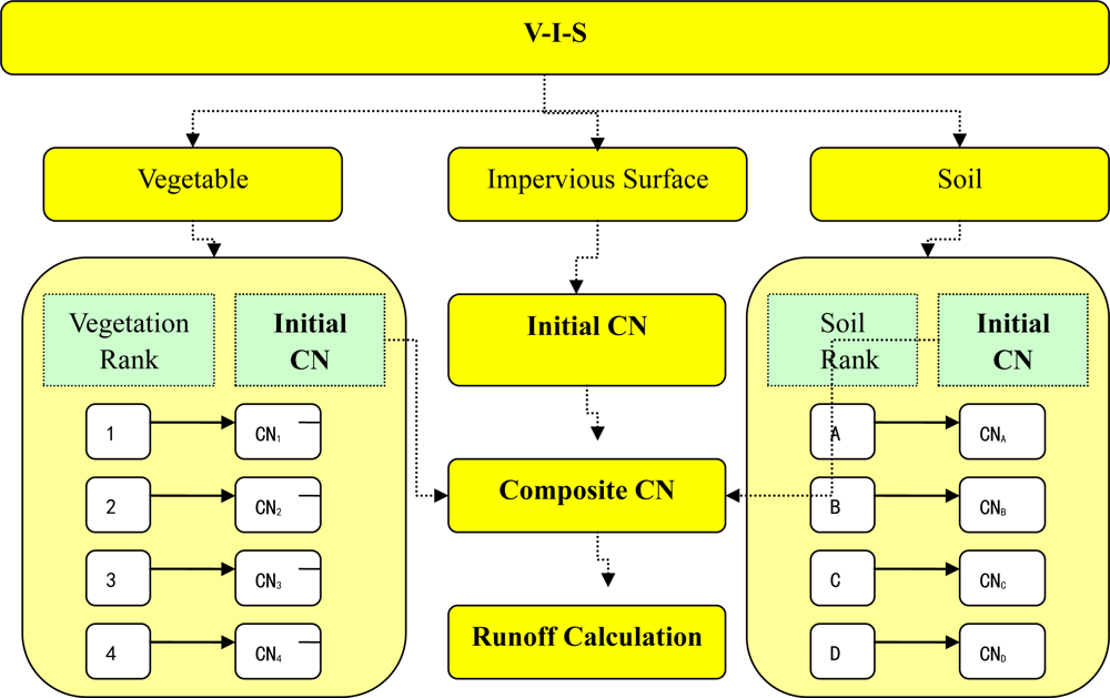
In this paper, a procedure is designed (Figure 2) to calculate composite CN, which includes four steps: (1) Obtaining NDVI values and classifying vegetation types. The NDVI values are grouped into four categories and each is assigned an initial CN value in reference to the TR-55 table; (2) Extracting V-I-S fraction images using the LSMA model. Vegetation, impervious surface and soil fractions are extracted from the satellite image; (3) Soil classification. Each type of soil is given an initial CN value in reference to the TR-55 based on its characteristics; and (4) Calculating composite CN. The composite CN is calculated as the weighted average of the initial CN values of vegetation, impervious surface and soil fractions. With this composite CN method, surface runoff is then simulated under the 57 mm and 81 mm precipitation for the study area.
In order to calculate composite CN of Guangzhou, we assume that any 30 m × 30 m pixel is considered as an independent drainage area and is comprised of impervious surface, vegetation and soil only. The formula of the composite CN calculation is as follows:
The values of NDVI are classified into four categories: (1) larger than 0.65 representing forest; (2) between 0.57 and 0.65 grass land, (3) between 0.4 and 0.57 farmland; and (4) less than 0.4 non-vegetation surfaces. Each category is further classified into several subclasses based on vegetation abundance derived from the vegetation fraction image. When vegetation fraction is larger than 0.75, vegetation is considered in healthy condition, while the fraction between 0.5 and 0.75 is considered in the fair condition and below 0.5 the poor condition. There are only one poor condition and good condition for farmland in the look-up table of TR-55. Hence, for farmland, we set the fraction value of 0.5 as the threshold to separate the good condition from the poor condition to determine CNV. The initial CN of each vegetation class is shown in Table 2.
4. Results
4.1. Vegetation, Impervious Surface and Soil Fractions
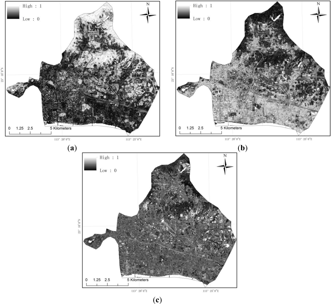
The LSMA method is applied to the Landsat TM image of 2009. Figure 3 shows the fraction images of impervious surface, vegetation and soil extracted from LSMA. The fraction value between 1 and 0 corresponded to the tonal variation from white color to black in the figure. It shows that large fractions of impervious surface are mainly located in the southern area, while vegetation is found to be more abundant in the northern area. Most of exposed soils are located in the eastern part of the study area. In addition, the accuracy assessment results indicate a good agreement between estimated results and the ground reference. The RSME for impervious surface, vegetation and soil fraction map yield 0.19, 0.21 and 0.35, respectively.
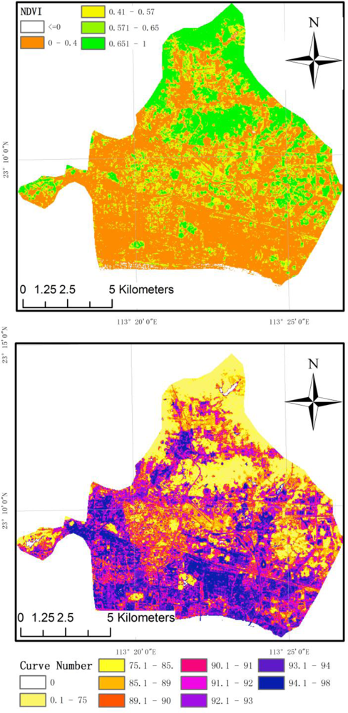
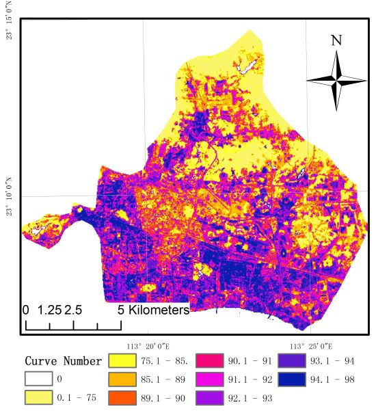
4.2. Mapping Composite CN
Composite CN is calculated according to Equation (7). The NDVI image and the composite CN image are shown in Figure 4. The composite CN values are divided into 10 categories, and the values larger than 75 are further examined because they affected the runoff significantly. Figure 4 shows that high values of NDVI are largely found in the northern part while lower values are in the southern part. In contrast, higher composite CN values tended to cluster in the south and lower values in the north. As Equation (7) shows, high percentage of impervious and low percentage of vegetation led to a high composite CN value, which is as anticipated based on background knowledge.
5. Case Study
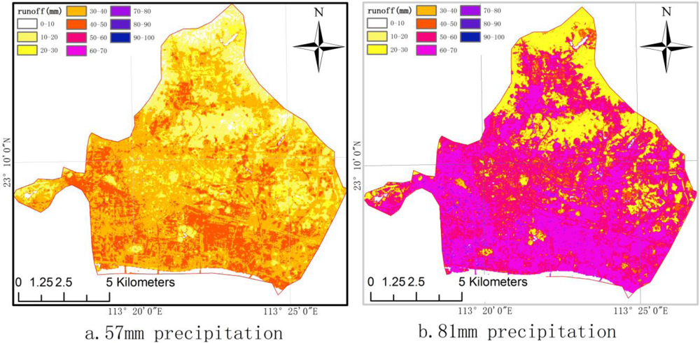
In Guangzhou, precipitation mainly occurs in the period from April to September, and is strongly impacted by typhoons and summer rainstorms. Daily precipitation up to 100 mm is common. In this study, we chose 57 mm and 81 mm of precipitation [28], which occur once in five years and once in ten years precipitation, respectively, to simulate surface runoff using the improved SCS-CN method. Because most of the rainfall in the urban city is transported through sewers rather than flowing onto the open terrain, the impacts of terrain roughness and elevation difference were not taken into account during the simulations.
Figure 5 shows the simulation results. The simulation with 57 mm precipitation is illustrated in the panel A of Figure 5. The highest runoff volume is found to be 51 mm, but most of the study areas observe runoff below 40 mm. By comparing with Figure 4, we find that the runoff volume is less than 31 mm in the areas that possessed NDVI value of greater than 0.57. However, under the scenario of 81 mm precipitation, the majority of study area is estimated to have a runoff volume of greater than 32 mm. This finding implies that when precipitation reached 81 mm, most of the study area would be threatened by surface flooding, especially in the southern part. Due to the lack of data, a real flood event is not included as a case study here.
6. Discussion
The SCS-CN model utilized in this study is to simulate surface runoff volume in the urban areas. Each pixel in the image is considered as a hydrologic response unit, and is decomposed into fractions of V-I-S. The composite CN of a pixel means the average CN of the whole pixel. This sub-pixel method of CN modeling is distinct from previous studies where each pixel is treated as a whole, i.e., per-pixel method (e.g., [39]).
Some previous researches calculate the CN based on land cover types and vegetation condition, while the soil types are neglected [40]. Hawkins (1998) and Canters et al. (2006) suggest that CN tables should only be used as a guideline, and actual CN and empirical relationships should be determined based on local and regional data [14,41].
In this study, the composite CN values are determined by the percentage of vegetation, impervious surface, and soil types. This procedure is straightforward. The main difficulty in its application lies in mapping the percentage of impervious surface, soil and vegetation via LSMA and determining the initial CN in reference to the look-up table of TR-55.
The LSMA model is based on a linear assumption in the spectra of all components within a pixel. However, the relationship becomes non-linear when multiple reflections occur. The selection of the end-members is a challenge, but critical for improving the fraction quality and classification accuracy. In addition, urban environment is examined under three conditions in TR-55, and there are more than ten classes under each condition. The selection of initial CN requires having a good knowledge of the study area. For example, it is necessary to know all the soil types in a study area and their characteristics before assigning the initial CN. Different soil types have different physical characteristics. These characteristics, like grain size and physical components, will affect water infiltration capability. As a result, biophysical characteristics of soil are important parameters for assigning initial CN. Likewise, soil moisture may be another critical parameter for assigning initial CN. Since the soil moisture content varies over time, it is difficult to be incorporated in the model. Besides, the TM image is acquired under the same weather condition, and thus we think that the study area had similar soil moisture conditions. In this study, we rely on the soil types for assigning initial CN values.
Impervious surface features include concrete, asphalt, metal and other artificial features, and water can hardly infiltrate. Thus, it is appropriate to assign a value of 98 for all impervious surface areas. NDVI is a simple vegetation index that can be used to analyze vegetation vigor from remote sensing images. The vegetation types may be classified according to the value of NDVI [20]. In this study, forest, grass, bush, farmland and none-vegetation area was classified via NDVI. This classification corresponded well to the vegetation types in the CN look-up table of the TR-55. It should be noted that NDVI may change over the seasons. Although most of the vegetations in Guangzhou are evergreen, the seasonal impact on computing the NDVI and the relationship between NDVI and vegetation cover cannot be ignored.
7. Conclusions
This paper presents a new method for computing the composite CN, which combines initial CNs of impervious surface, vegetation and soil. This improved method is built based on the successful runoff estimating method, SCS-CN. The calculation of composite CN is the key to a successful SCS-CN modeling. This key variable has frequently been obtained from the look-up table of TR-55. However, due to the complexity of land surface features in urban environments, the CN in the TR-55 cannot be applied to all surface types. Therefore, we developed an innovative method to make the SCS-CN method easy to use. The strength of the improved method is that the calculation incorporated the percentages of vegetation, soil, and impervious surface in the urban areas.
In addition, in order to test the feasibility and effectiveness of this improved method, surface runoff is simulated under the scenario of 57 and 81 mm precipitation for the Tianhe District of Guangzhou City and the depth of the runoff is mapped respectively. The result demonstrated that the improved SCS-CN method by using remote sensing variables to estimate runoff is convenient and effective. The CN map, especially the surface runoff map, provided a useful tool for storm management for the local governments.
Acknowledgments
This work is supported by National Nature Science Foundation of China (Grant No: 41201432). The support from the research program of LREIS (O88RA900KA) and a key project for the strategic science plan in IGSNRR (2012ZD010) are also acknowledged. Three anonymous reviewers provided constructive comments and suggestions, which helped improve the manuscript.
References
- Burnash, R.; Singh, V. The NWS River Forecast System-Catchment Modeling. In Computer Models of Watershed Hydrology; Singh, V.P., Ed.; Water Resources Publications, LLC Company: Littleton, CO, USA, 1995; pp. 311–366. [Google Scholar]
- Sugawara, M. Tank Model. In Computer Models of Watershed Hydrology; Singh, V.P., Ed.; Water Resources Publications, LLC Company: Littleton, CO, USA, 1995; pp. 165–214. [Google Scholar]
- Bergstro m, S. The HBV Model. In Computer Models of Watershed Hydrology; Singh, V.P., Ed.; Water Resources Publications, LLC Company: Littleton, CO, USA, 1995; pp. 443–476. [Google Scholar]
- Nielsen, S.A.; Hansen, E. Numerical simulation of the rainfall runoff process on a daily basis. Nordic. Hydrol 1973, 4, 171–190. [Google Scholar]
- Havnø, K.; Madsen, M.N.; Dørge, J. MIKE 11—A Generalized River Modelling Package. In Computer Models of Watershed Hydrology; Singh, V.P., Ed.; Water Resources Publications, LLC Company: Littleton, CO, USA, 1995; pp. 733–782. [Google Scholar]
- Boughton, W. A review of the USDA SCS curve number method. Soil Res 1989, 27, 511–523. [Google Scholar]
- On-Site Wastewater Management Guidance Manual; North Carolina Division of Environmental Health-The Public Water Supply Section: Raleigh, NC, USA, 1996.
- Kousari, M.R.; Malekinezhad, H.; Ahani, H.; Zarch, M.A.A. Sensitivity analysis and impact quantification of the main factors affecting peak discharge in the SCS curve number method: An analysis of Iranian watersheds. Quat. Int 2010, 226, 66–74. [Google Scholar]
- Knisel, W.G. CREAMS: A Field Scale Model for Chemicals, Runoff, and Erosion from Agricultural Management Systems; Conservation Research Report No. 26; US Department of Agriculture-Sea Agrcultural Research: Beaumont, TX, USA, 1980. [Google Scholar]
- Wight, J.R.; Skiles, J.W. SPUR: Simulation of Production and Utilization of Rangelands. Documentation and Users Guide; US Department of Agriculture-Agricultural Research Service: Washington, DC, USA, 1987; p. 372. [Google Scholar]
- Young, D.F.; Carleton, J.N. Implementation of a probabilistic curve number method in the PRZM runoff model. Environ. Modell. Softw 2006, 21, 1172–1179. [Google Scholar]
- Cronshey, R.G.; Roberts, R.T.; Miller, N. Urban Hydrology for Small Watersheds (TR-55 Rev.); Hydraulics and Hydrology in the Small Computer Age: Proceedings of the Specialty Conference, Lake Buena Vista, Florida, August 12–17, 1985, Waldrop, W.R., Ed.; Hydrology Division-American Society of Civil Engineers: Reston, VA, USA, 1985. [Google Scholar]
- Hong, Y.; Adler, R.F. Estimation of global SCS curve numbers using satellite remote sensing and geospatial data. Int. J. Remote Sens 2008, 29, 471–477. [Google Scholar]
- Canters, F.; Chormanski, J.; Van de Voorde, T.; Batelaan, O. Effects of Different Methods for Estimating Impervious Surface cover on Runoff Estimation at Catchment Level. Proceedings of 7th International Symposium on Spatial Accuracy Assessment in Natural Resources and Environmental Sciences, Lisbon, Portugal, 5–7 July 2006; pp. 557–566.
- Reistetter, J.A.; Russell, M. High-resolution land cover datasets, composite curve numbers, and storm water retention in the Tampa Bay, FL region. Appl. Geogr 2011, 31, 740–747. [Google Scholar]
- Dutta, S.; Mishra, A.; Kar, S.; Panigrahy, S. Estimating spatial curve number for hydrologic response analysis of a small watershed. J. Spat. Hydrol 2006, 6, 57–67. [Google Scholar]
- Ludlow, C. Flood Modeling in a Data-Poor Region: A Satellite Data-Supported Flood Model for Accra, Ghana. Proceedings of Annual Meeting of the Association for American Geographers, Las Vegas, NV, USA, 22–27 March 2009.
- Ridd, M.K. Exploring a V-I-S (vegetation-impervious surface-soil) model for urban ecosystem analysis through remote sensing: Comparative anatomy for cities. Int. J. Remote Sens 1995, 16, 2165–2185. [Google Scholar]
- Lu, D.S.; Weng, Q.H. Extraction of urban impervious surfaces from an IKONOS image. Int. J. Remote Sens 2009, 30, 1297–1311. [Google Scholar]
- Wu, C.S. Quantifying high-resolution impervious surfaces using spectral mixture analysis. Int. J. Remote Sens 2009, 30, 2915–2932. [Google Scholar]
- Weng, Q.H.; Hu, X.F.; Lu, D.S. Extracting impervious surfaces from medium spatial resolution multispectral and hyperspectral imagery: a comparison. Int. J. Remote Sens 2008, 29, 3209–3232. [Google Scholar]
- Deng, Y.B.; Fan, F.L.; Chen, R.R. Extraction and analysis of impervious surfaces based on a Spectral un-mixing method using Pearl River delta of China Landsat TM/ETM plus imagery from 1998 to 2008. Sensors 2012, 12, 1846–1862. [Google Scholar]
- Wu, C.S.; Murray, A.T. Estimating impervious surface distribution by spectral mixture analysis. Remote Sens. Environ 2003, 84, 493–505. [Google Scholar]
- Yang, J.S.; Artigas, F.J. Estimating impervious surfaces area of urban watersheds using ASTER data. J. Environ. Inform 2008, 12, 1–8. [Google Scholar]
- Elvidge, C.D.; Tuttle, B.T.; Sutton, P.S.; Baugh, K.E.; Howard, A.T.; Milesi, C.; Bhaduri, B.L.; Nemani, R. Global distribution and density of constructed impervious surfaces. Sensors 2007, 7, 1962–1979. [Google Scholar]
- Jiang, L.M.; Liao, M.S.; Lin, H.; Yang, L.M. Synergistic use of optical and InSAR data for urban impervious surface mapping: a case study in Hong Kong. Int. J. Remote Sens 2009, 30, 2781–2796. [Google Scholar]
- Lu, D.S.; Weng, Q.H. Spectral mixture analysis of the urban landscape in Indianapolis with landsat ETM plus imagery. Photogramm. Eng. Remote Sensing 2004, 70, 1053–1062. [Google Scholar]
- Quan, R.; Liu, M.; Zhang, L.; Lu, M.; Wang, J.; Niu, H.; Xu, S. Exposure assessment of rainstorm waterlogging on buildings in central urban area of Shanghai based on scenario simulation. Sci. Geogr. Sin 2011, 2, 148–152. [Google Scholar]
- Wu, S.; Hu, Y.; Dai, J.; Jiang, C. A study on creation of database for a Guangdong Province soil resource information system. J. S. China Agric. U 2001, 4, 22–25. [Google Scholar]
- Roberts, D.A.; Gardner, M.; Church, R.; Ustin, S.; Scheer, G.; Green, R.O. Mapping chaparral in the Santa Monica Mountains using multiple endmember spectral mixture models. Remote Sens. Environ 1998, 65, 267–279. [Google Scholar]
- Smith, M.O.; Ustin, S.L.; Adams, J.B.; Gillespie, A.R. Vegetation in deserts: I. A regional measure of abundance from multispectral images. Remote Sens. Environ 1990, 31, 1–26. [Google Scholar]
- Mustard, J.F.; Sunshine, J.M. Spectral Analysis for Earth Science: Investigations Using Remote Sensing Data. In Remote Sensing for the Earth Sciences: Manual of Remote Sensing; Rencz, A.N., Ed.; John Wiley & Sons: New York, NY, USA, 1999; Volume 3, pp. 251–307. [Google Scholar]
- Adams, J.B.; Sabol, D.E.; Kapos, V.; Almeida, R.; Roberts, D.A.; Smith, M.O.; Gillespie, A.R. Classification of multispectral images based on fractions of endmembers—Application to land-cover change in the brazilian amazon. Remote Sens. Environ 1995, 52, 137–154. [Google Scholar]
- Green, A.A.; Berman, M.; Switzer, P.; Craig, M.D. A transformation for ordering multispectral data in terms of image quality with implications for noise removal. IEEE Trans. Geosci. Remote Sens 1988, 26, 65–74. [Google Scholar]
- McFeeters, S.K. The use of the normalized difference water index (NDWI) in the delineation of open water features. Int. J. Remote Sens 1996, 17, 1425–1432. [Google Scholar]
- Weng, Q.H.; Hu, X.F. Medium spatial resolution satellite imagery for estimating and mapping urban impervious surfaces using LSMA and ANN. IEEE Trans. Geosci. Remote Sens 2008, 46, 2397–2406. [Google Scholar]
- Ponce, V.M.; Hawkins, R.H. Runoff curve number: Has it reached maturity? J. Hydrol. Eng 1996, 1, 11–19. [Google Scholar]
- Silveira, L.; Charbonnier, F.; Genta, J.L. The antecedent soil moisture condition of the curve number procedure. Hydrol. Sci. J 2000, 45, 3–12. [Google Scholar]
- Weng, Q.H. Modeling urban growth effects on surface runoff with the integration of remote sensing and GIS. Environ. Manage 2001, 28, 737–748. [Google Scholar]
- Kumar, P.; TIWART, K.; Pal, D. Establishing SCS runoff curve number from IRS digital data base. J Indian Soc. Remote 1991, 19, 245–252. [Google Scholar]
- Hawkins, R.H. Local Sources for Runoff Curve Numbers. Proceedings of 11th Annual Symposium of the Arizona Hydrological Society, Tucson, AZ, USA, 23–26 September 1998.


| Soil Type | CNs | Class |
|---|---|---|
| Paddy soil | 94 | D |
| Deposited soil | 91 | C |
| Red soil | 86 | B |
| Aquic soil | 91 | C |
| Vegetation | NDVI | Vegetation Vigor | CN | |||
|---|---|---|---|---|---|---|
| A | B | C | D | |||
| Forest | NDVI > 0.65 | Poor: V < 50% | 45 | 66 | 77 | 83 |
| Fair: 50% < V < 75% | 36 | 60 | 73 | 79 | ||
| Good: V > 75% | 30 | 55 | 70 | 77 | ||
| Grass and Bush | 0.57 < NDVI < 0.65 | Poor: V < 50% | 57 | 73 | 82 | 86 |
| Fair: 50% < V < 75% | 43 | 65 | 76 | 82 | ||
| Good: V > 75% | 32 | 58 | 72 | 79 | ||
| Farmland | 0.4 < NDVI < 0.57 | Poor: V < 50% | 72 | 81 | 88 | 91 |
| Good: V > 50% | 67 | 78 | 85 | 89 | ||
| None-Vegetated | NDVI < 0.4 | 59 | 74 | 82 | 86 | |
Share and Cite
Fan, F.; Deng, Y.; Hu, X.; Weng, Q. Estimating Composite Curve Number Using an Improved SCS-CN Method with Remotely Sensed Variables in Guangzhou, China. Remote Sens. 2013, 5, 1425-1438. https://doi.org/10.3390/rs5031425
Fan F, Deng Y, Hu X, Weng Q. Estimating Composite Curve Number Using an Improved SCS-CN Method with Remotely Sensed Variables in Guangzhou, China. Remote Sensing. 2013; 5(3):1425-1438. https://doi.org/10.3390/rs5031425
Chicago/Turabian StyleFan, Fenglei, Yingbin Deng, Xuefei Hu, and Qihao Weng. 2013. "Estimating Composite Curve Number Using an Improved SCS-CN Method with Remotely Sensed Variables in Guangzhou, China" Remote Sensing 5, no. 3: 1425-1438. https://doi.org/10.3390/rs5031425