Investigating the Relationship between X-Band SAR Data from COSMO-SkyMed Satellite and NDVI for LAI Detection


Abstract
: Monitoring spatial and temporal variability of vegetation is important to manage land and water resources, with significant impact on the sustainability of modern agriculture. Cloud cover noticeably reduces the temporal resolution of retrievals based on optical data. COSMO-SkyMed (the new Italian Synthetic Aperture RADAR-SAR) opened new opportunities to develop agro-hydrological applications. Indeed, it represents a valuable source of data for operational use, due to the high spatial and temporal resolutions. Although X-band is not the most suitable to model agricultural and hydrological processes, an assessment of vegetation development can be achieved combing optical vegetation indices (VIs) and SAR backscattering data. In this paper, a correlation analysis has been performed between the crossed horizontal-vertical (HV) backscattering (σ°HV) and optical VIs (VIopt) on several plots. The correlation analysis was based on incidence angle, spatial resolution and polarization mode. Results have shown that temporal changes of σ°HV (Δσ°HV) acquired with high angles (off nadir angle; θ > 40°) best correlates with variations of VIopt (ΔVI). The correlation between ΔVI and Δσ°HV has been shown to be temporally robust. Based on this experimental evidence, a model to infer a VI from σ° (VISAR) at the time, ti+ 1, once known, the VIopt at a reference time, ti, and Δσ°HV between times, ti + 1 and ti, was implemented and verified. This approach has led to the development and validation of an algorithm for coupling a VIopt derived from DEIMOS-1 images and σ°HV. The study was carried out over the Sele plain (Campania, Italy), which is mainly characterized by herbaceous crops. In situ measurements included leaf area index (LAI), which were collected weekly between August and September 2011 in 25 sites, simultaneously to COSMO-SkyMed (CSK) and DEIMOS-1 imaging. Results confirm that VISAR obtained using the combined model is able to increase the feasibility of operational satellite-based products for supporting agricultural practices. This study is carried out in the framework of the COSMOLAND project (Use of COSMO-SkyMed SAR data for LAND cover classification and surface parameters retrieval over agricultural sites) funded by the Italian Space Agency (ASI).1. Introduction
Earth observation (EO) is more and more used to manage land and water resources for agricultural applications, such as leaf water potential [1,2], soil water content [3–7], irrigation water management [8–10] and flood prediction [11–13]. Diversely from optical imaging, the temporal resolution of observations from active sensors, such as SAR, is not limited by sky cloudiness; if carefully validated, it may be used in combination with thermal and optical imageries to provide a more continuous monitoring of land surfaces. Several new SAR missions have been launched or planned: ALOS-PALSAR (Japan); COSMO-SkyMed 1 and 2 (Italy); TerraSAR-X and TerraSAR-X2 (Germany); SeoSAR PAZ 1 and 2 (Spain); Sentinel 1 (European Space Agency); Radarsat RCM (Canada); Kompsat 5 (Korea). These new SAR missions (acquiring at X-, C- and L-bands) are characterized by dual polarization capability, a short revisit time (from 12 h to ∼10 days) and high spatial resolution (<20 m), which could provide suitable data for operative crop monitoring [14,15].
Numerous studies using either airborne or spaceborne platforms exploit SAR data for biomass estimation [16–19]. SAR backscattering is sometimes strongly correlated with forest biomass, particularly characterized by low-medium fractional cover and at lower frequencies (P- and L-band) [20–22].
Mapping vegetation using X-band data has limitations [23], because radiation at X-band penetrates only the upper part of the canopy; thus, radar backscattering is only related to the top layer and the crown.
Although X-band is not the most suitable for agro-hydrological applications, vegetation can be monitored combing optical and SAR backscattering data.
Recently, some research efforts have been carried out in addressing biomass or vegetation water content [24] using X-band images. However, the use of SAR data to reproduce ‘optical’ vegetation indices, such as the normalized difference vegetation index (NDVI) and leaf area index (LAI), is an important task, because these are key-input data in both mass and energy exchange models of soil-vegetation-atmosphere systems (e.g., SWAP and SEBAL, et similia).
COSMO-SkyMed, given its high temporal and spatial resolution, opened new opportunities for an operative monitoring in this framework. This paper explores the possibility of coupling SAR and optical images for assessing a new type of VI, as resulting from the project “Use of COSMO-SkyMed data for LANDcover classification and surface parameters retrieval over agricultural sites” (COSMOLAND), funded by the Italian Space Agency (ASI) [25].
The specific objectives of the COSMOLAND project were: (i) improving, tailoring and validating methods and algorithms for land-cover classification and surface parameter retrieval (including LAI) at the regional scale, using COSMO-SkyMed X-band SAR (CSK) data, as well as observations with optical passive sensors; and (ii) integrating the output of these algorithms into existing hydrological/crop growth models. This research was carried out in the framework of the first objective.
2. Test Site, Dataset and Methods
2.1. Test Site
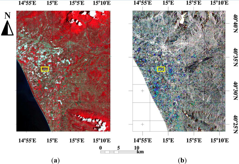
The Sele plain covers an area of ≈500 km2 and is located in the Campania region (Southern Italy) (Figure 1). The main crops are maize, forages, potatoes, vegetables, peaches, apricot and pear, which are irrigated from April to October.
The experimental farm “Improsta” is located in the Sele plain, approximately at 14°58′E, 40°33′N (see rectangle in Figure 1), and is managed by the Regional Administration of Campania. Within it, herbaceous crops, such as maize and alfalfa, are continuously monitored in several plots for research purposes and agricultural extension services.
2.2. Dataset
The dataset includes CSK and optical images (in the visible and near infrared ranges) and in situ LAI.
2.2.1. Satellite Images
Active microwave (SAR). The CSK mission, developed in cooperation between ASI and the Italian Defense Ministry, is planned as a constellation of four satellites, carrying X-band SAR with right and left looking imaging capabilities, an incidence angle ranging between 20° and 60°and a revisit time of 12 h in the worst case.
The antenna was designed to implement three different operation modes: (i) spotlight, for metric spatial resolution over an area footprint of 100 km2, in single polarization; (ii) stripmap, for decametric resolution covering areas from 900 to 1,600 km2, with dual polarization capability (the so-called PingPong configuration); (iii) scanSAR, for tens to hundreds meter resolution over areas ranging from 10,000 to 40,000 km2.
Seventeen spotlight (SP) and PingPong (PP) images were acquired between 4 August and 5 September 2011 (Table 1):
- 7 Spotlight images (vertical-vertical (VV) polarization, 0.5 m spatial resolution and two different mean incidence angles: 27°(SPlow) and 41° (SPhigh));
- 10 Stripmap PingPong images (HH and HV polarizations and 10 m spatial resolution; mean angles: 27° (PPlow) and 46° (PPhigh)).
Passive optical. DEIMOS-1 is a low Earth quasi-polar sun synchronous satellite, launched on 29 July 2009 and carrying on board the SLIM6 instrument (Surrey Linear Imager Multispectral 6 channels) having 3 spectral bands: near-infrared (NIR, 0.77–0.90 μm), red (R, 0.63–0.69 μm) and green (G, 0.52–0.60 μm).
The DEIMOS-1 Mission, fully owned and operated by DEIMOS Imaging S.L., offers a new source of geospatial imagery at medium spatial resolution (22 m) covering large areas with a swath of approximately 600 km. DEIMOS-1 satellite provides a revisit time of 2–3 days, with a competitive cost per unit km2, thus making it particularly suitable for operational applications (e.g., precision farming).
Five DEIMOS-1 optical images have been collected between 3 August and 7 September in the framework of the project IRRISAT [26]. Figure 2 shows a CIR DEIMOS-1 color composite subset of the Improsta farm. Preliminary processing included: atmospheric correction based on MODTRAN and library reference spectra of vegetation and NDVI retrieval.
2.2.2. In situ LAI
LAI (m2·m−2) has been collected weekly between 1 August and 12 September with a LICOR LAI-2000 Plant Canopy Analyzer [27]; the dataset was acquired within 25 plots of corn and alfalfa. In particular, the average LAI is retrieved at sunrise from three measurement repetitions of eight below-canopy readings each. Moreover, an opaque cover (view cap) with an open wedge of 180° was used to avoid the influence of neighboring obstacles (e.g., the operator). This measurement protocol allowed to determine statistically meaningful LAI values characterized by a low ratio between SEL (standard error of the LAI) and LAI (SEL/LAI ranged between ≈0.02 and ≈0.1); thus, the actual LAI should be within ±10% of the LAI sample mean.
Measured LAI ranged between 0.36 and 5.35 m2·m−2 with an average value of 2.39 m2·m−2. In situ LAI have been used for producing LAI maps from DEIMOS images by applying an exponential relationship with NDVI, i.e., 0.172e3.64NDVI[28]. The calibration of the NDVI vs. LAI relationship resulted in a determination coefficient, r2 = 0.91, with a standard error (S.E.) of 0.50 m2·m−2. Hereinafter, we refer to LAI as the estimated values from DEIMOS images.
2.3. Methods
Pre-processing of CSK images included: (a) backscattering calibration and (b) speckle reduction. Speckle reduction has been achieved by applying a multi-temporal filter operator [29] with a 7 × 7 kernel. The appropriate spatial resolution has been evaluated through a geo-statistical analysis based on the Moran’s index [30] and the eight directions “Queen case” approach.
The multi-temporal filtering has been chosen to fully exploit both space and time dimensions to achieve the required equivalent number of looks (ENL), thus obtaining a satisfactory speckle reduction [31,32].
The resulting speckle index was on average 0.12 compared to 0.20 in the original images. Moreover, the chosen filter preserves the spatial resolution of the input data that is still suitable for crop monitoring and similar to the spatial resolution of the optical images.
Hereinafter, σCSK is used to indicate σ°HV, σ°HH, σ°VV, as well as the depolarization difference, dpr = σ°HV − σ°HH (dB).
This latter is sensitive either to bare soil roughness or to crop height; indeed, variations of these surface characteristics determine a higher increase of σ°HV compared to that of σ°HH [33,34].
The comparison between σCSK and VIs was made following two different approaches:
image segmentation and comparison of average values for each class;
temporal variation within small homogeneous areas.
The relationship between σCSK and VIs is to be researched in space and time. The first approach investigates the space variability for fixed time and vice versa; the second approach examines the temporal variability for given space intervals.
To this aim, we used a total of 8 σCSK sets (σ°HV, σ°HH, σ°VV and dpr collected at both low and high incidence angles) and 2 VI sets (NDVI and LAI). For each σCSK image, we have considered the nearest VI.
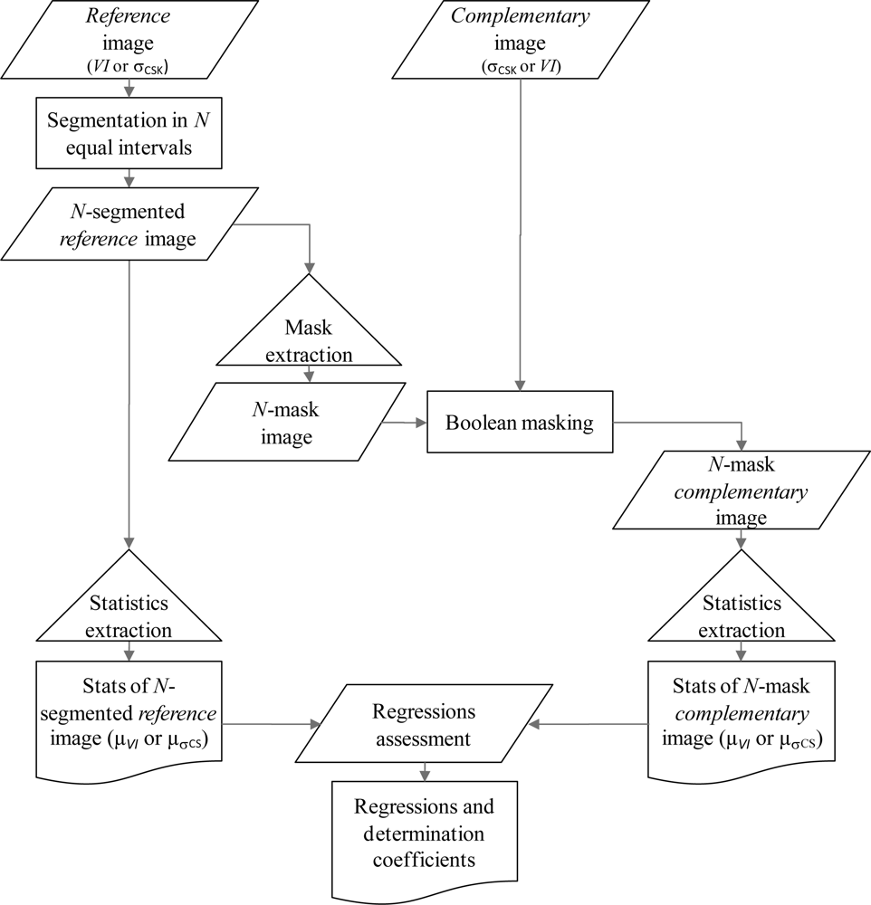
In the first approach, the procedure has been applied with two different schemes (Figure 3):
- The first scheme uses VI as the reference image and σCSK as the complementary one;
- Conversely, the second scheme uses σCSK as the reference image and VI as complementary.
Reference and complementary images are assumed as synchronous.
In each scheme, the reference image has been segmented into N-equal intervals (applying the equal interval data classification) and for each interval mean, and standard deviation values have been extracted. The segmented reference image is then used to create a Boolean mask for identifying corresponding pixels of the complementary image and, for each subset of the complementary image, the same statistics have then been calculated. Finally, the statistics of reference and complementary images have been compared to investigate any reciprocal relationship between average values and data variability of σCSK and VI.
In the second approach, a diachronic analysis between variation of VI and σCSK, namely ΔVI and ΔσCSK, has been carried out within a set of homogeneous areas to investigate the influence of canopy growth on solar energy absorption/reflection and microwave backscattering. Once selected, for 30 homogeneous areas, characterized by low, moderate and high temporal ΔVI, the corresponding ΔσCSK has been derived.
An empirical relationship has been sought between the two variations to be successively applied to the whole image. The results have been validated by using in situ data taken at the Improsta farm.
3. Results
Approach 1: Image Segmentation
From the different VI and σCSK datasets considered in scheme 1, the existence of a general exponential relationship between the averages of VI and the corresponding σCSK value was found:
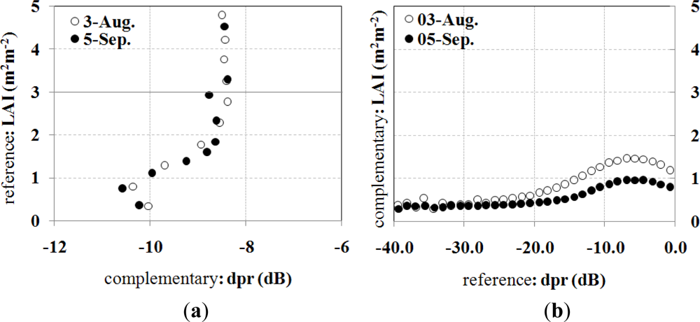
Figure 4(a,b) refers to the application of schemes 1 and 2, respectively. In Figure 4(a), VI is the reference image, whilst in Figure 4(b), σCSK has been used as the reference, according to the scheme 2. In scheme 1, best fitting (N = 10; r2 ∼ 0.79, Figure 4(a)) resulted when considering LAI for VI and dpr for σCSK collected at high angles only (dprhigh), thus reducing the available dataset to five couples of DEIMOS-1 and CSK images. The choice of N in the segmentation did not influence the results if N is greater than 10. The relationship is applicable if LAI ranges between 0.5 and 3. For LAI < 0.5, the soil roughness is strong enough to influence the backscattering; diversely, for LAI > 3, the relationship tends to a vertical asymptote, which can be considered as the upper limit of validity.
Other VI-σCSK returned lower correlations compared to the findings of Figure 4(a). As a consequence, SP images (acquired in co-polarized mode only) and PPlow have not been considered for further setting up and/or calibrating the model. A discrepancy in the backscattering levels between SP and PP has been also found.
In particular, the SP vs. PP revealed only a moderate r2 (∼0.59); this is due both to differences in the look angles (21°and 41°for SP, 27°and 46°for PP) and to differences of the image generation between PP and SP having great influences, especially regarding the focusing azimuth process, and thus, in the backscattering level.
The relationship (1) was in line with expectations deriving from a physical interpretation of the backscattering phenomenon, with more vegetation showing higher difference between cross-polarized and co-polarized backscattering.
Furthermore, the disaggregation between two different dates showed the relationship to be almost temporally invariant.
However, relationship (1) has been retrieved between average values of both VI and σCSK variables. Actual standard deviation values of σCSK found for each VI interval are very high, meaning that the variability of the independent variable cannot be fully explained by that observed for the dependent variable.
For this reason, the average values of the independent variable are actually constrained in a limited range. These results are ever observable between variables that are moderately or coarsely pixel-wise correlated (as occurring in this case).
Indeed, the standard deviation values of dpr (dprst.dev) within LAI intervals are high, especially for the lowest LAI ranges (dprst.dev ranges from 3.7 to 3 dB for 3 August and it ranges from 5.5 to 2.8 dB for 5 September). This means that an average dpr value (dpravg) of −10 dB represent dpr values ranging from −16 to −3 dB (considering two-times the dprst.dev).
For the above-mentioned reasons, scheme 2, which was based on the segmentation of σCSK, did not confirm, as expected, the previous finding (Figure 4(b)). Different σCSK classes produced similar VI averages, with significant differences for distinct acquisition dates.
Furthermore, we notice that the maximum LAI observed in the different intervals of backscattering used for the segmentation is 1–1.5 m2·m−2 (Figure 4(b)), that is comparable (i.e., the average plus the standard deviation is up to 2.7 m2·m−2) to the maximum value of 3 m2·m−2, which is possible to infer according to scheme 1 (Figure 4(a)). It means that the segmentation based on backscattering determines areas characterized by a larger variability of LAI compared to the opposite scheme 1. This highlights that it is not possible to apply a relationship similar to Equation (2) to infer LAIavg starting from average σCSK values.
One reason for these findings could be due to the effect of residual speckle, even after the de-speckling pre-processing, thus leading to the evidence that dpr average variability cannot be fully explained by LAI averages and vice versa.
A larger kernel could be used to further reduce the speckle, but this choice is limited by the average size of the agricultural plots of the Sele plain (land heterogeneity).
Approach 2: Temporal Variations
In the second approach, the relationship between the variation of both σCSK and VIs between two consecutive acquisitions has been analyzed (ΔVI and ΔσCSK, respectively).
Firstly, we have selected a limited subset of the image, corresponding to homogeneous vegetation cover (i.e., characterized by low coefficient of variation) and different average LAI values. We have analyzed the variation of both VI and σCSK between a reference date (3 August) and subsequent acquisitions; this leads to four different sets of ΔVI and ΔσCSK. Another two additional sets of variation have been calculated considering as the reference date the acquisition of 19 August and the two subsequent images.
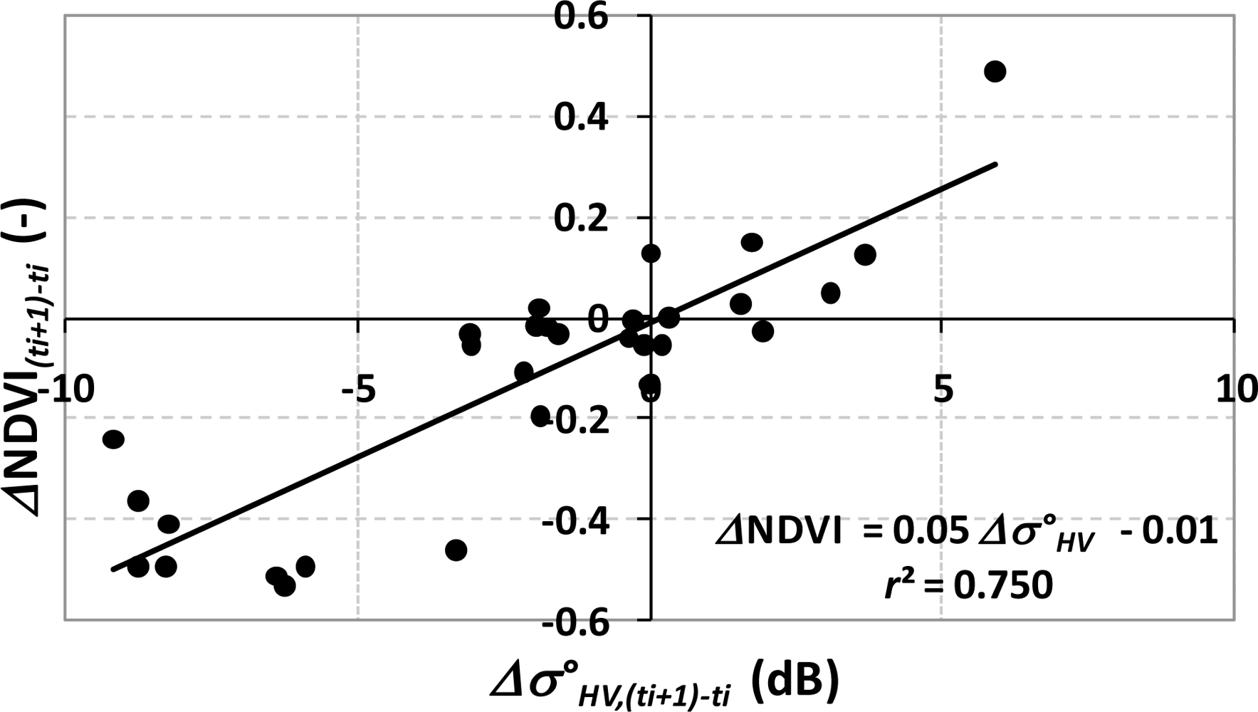
Among all the possible couples of ΔVI and ΔσCSK, the best fitting was found when considering NDVI for VI and σ°HV,high (r2 = 0.75), the latter corresponding to the acquisition mode PPhigh (Section 2.2.1), hereinafter σ°HV for the sake of brevity.
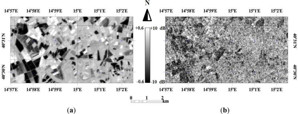
This result confirms previous findings, i.e., σ°pq (backscattering acquired in cross-polarization) is more sensitive than like-polarized backscattering, σ°pp, to the temporal variations of vegetation biomass [35]. Figure 5 shows, as an example, the spatial distributions of ΔNDVI(ti + 1) − ti and Δσ°HV,(ti + 1) − ti between times ti + 1 = 5 September and ti = 3 August (ΔNDVI(ti + 1) − ti = NDVIti + 1 − NDVIti and Δσ°HV,(ti + 1) − ti = σHV,(ti + 1) − σ°HV,ti).
Knowing NDVIti at a reference time, ti, and the variation of backscattering, Δσ°HV,(ti + 1) − ti, between times, ti + 1 and ti, it is then possible to infer NDVIti + 1 by means of a linear relationship:
Within the above relationship (2), NDVIti accounts for the spatial pattern, while (γ·Δσ°HV,(ti + 1) − ti+ δ) describes its temporal variability. In other words, the variability of the two sets, NDVI and σ°CSK, is determined by different interactions between the surface and the active/passive signals, whilst the response in two consecutive images shows a similar behavior (linear proportionality in increments or decrements). This procedure does not require a preliminary segmentation of the image, as in Approach (1). Figure 6 shows the relationship between ΔNDVI(ti + 1) − ti and Δσ°HV,(ti + 1) − ti using the calibration dataset.
Once Equation (2) has been applied to the whole study area, the method has been validated on a subset of homogeneous areas. These areas were selected by classifying the NDVI time series by using a k-means algorithm [36]. Thus, five clusters of NDVI showing similar temporal behavior were determined.
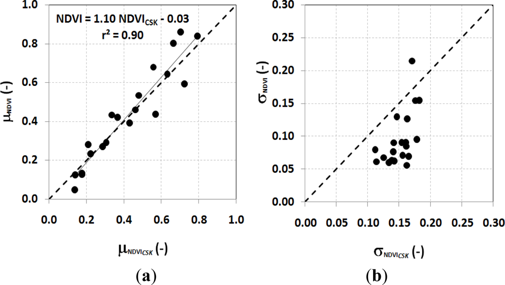
In Figure 7, we compare average and st.dev values of NDVI (Figure 7(a,b), respectively) retrieved from Equation (3), NDVICSK and the corresponding original ones from DEIMOS images. The average values, μNDVICSK vs. μNDVI, are significantly correlated (r2 ≈ 0.90, m ≈ 1.10, q ≈ 0.03); as expected, the standard deviation of σNDVICSK is higher than σNDVI.
Table 2 reports the temporal averages, temporal st.dev and S.E. of the NDVICSK vs. NDVI for corn and alfalfa u.i. of the Improsta farm. The S.E. of the NDVI ranges between 0.05 and 0.21 (−) over corn plots, whereas it ranges between 0.18 and 0.26 (−) over alfalfa.
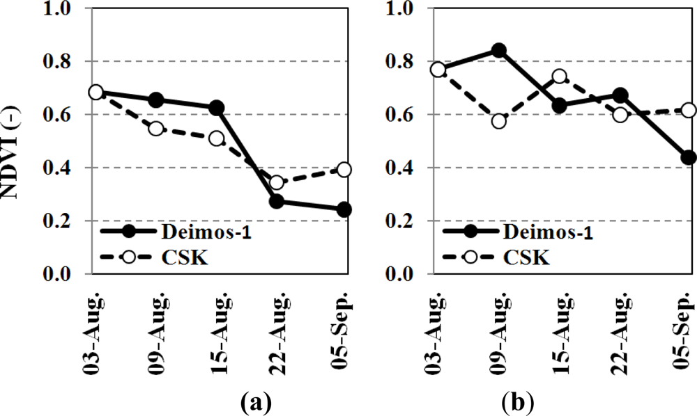
Figure 8 shows the temporal behavior of NDVI and NDVICSK for a corn and an alfalfa plot of the Improsta farm (Figure 3). NDVICSK has been derived using the acquisition of 3 August as the reference time, ti.
Better agreement between NDVICSK and NDVI has been found for corn rather than alfalfa plots, especially for the second acquisition date; this result has been also confirmed for other irrigation units. NDVICSK vs. NDVI on corn was characterized by r2 ≈ 0.98; NDVI is slightly overestimated by NDVICSK for NDVICSK > 0.67 (m ≈ 1.38, q ≈ −0.25), whereas the dispersion in alfalfa plots has a lower r2 (≈0.66), and the linear regression line has a lower offset (m ≈ 0.83, q ≈ 0.14).
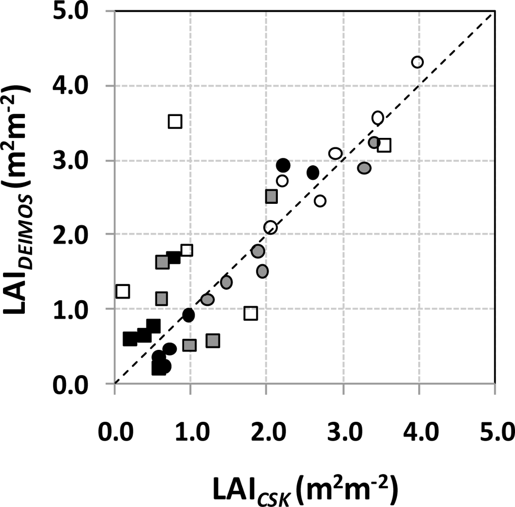
Successively, we have applied the exponential empirical relationship defined in Section 2.2.2 to NDVICSK to retrieve LAICSK. Figure 9 shows the correlation between LAI and LAICSK for alfalfa and corn u.i.; dots represent minima, maxima and averages values (during the period 3 August–5 September).
According to NDVI, again, LAICSK vs. LAI on corn was characterized by high r2 (≈0.95); LAI is slightly underestimated when LAICSK > 0.04 m2·m−2 (m ≈ 1.04, q ≈ 0.12), whereas the dispersion on alfalfa has lower r2 (≈0.31), and LAI is slightly underestimated by LAICSK on the whole range of variability (m ≈ 0.64, q ≈ 0.69).
Finally, Table 3 reports field temporal averages, temporal st.dev and S.E. of the LAICSK vs. LAI for corn and alfalfa. The S.E. of the LAI ranges between 0.29 and 0.84 (m2·m−2) over corn plots, whereas it is higher for alfalfa (up to 1.41 m2·m−2). The lower agreement for alfalfa is probably related to irrigation, which could affect more strongly the backscattering of this kind of canopy. Unluckily, in situ measures of soil water content and soil surface roughness were not available to assess how these variables affect the proposed procedure. However, at the X-band, the backscattering results mainly from the upper part of the canopy and leaves, with little contribution due to the underlying soil surface [37–39].
4. Conclusions
The possibility of using backscattering SAR images to assess vegetation development and LAI has been investigated within this paper, by comparing optical and X-band SAR images from the novel COSMO-SkyMed constellation, which has a great potential in terms of spatial and temporal resolution. LAI maps derived from DEIMOS optical sensors have been used as the reference.
Areas with a similar value of LAI, in the range 0–3 m2·m−2, respond in a similar way to X-band backscattering, as shown in the first part of the study; an empirical relationship has been observed between average LAI and average backscattering depolarization difference. However, the large variability of backscattering within a cluster of pixels with similar LAI values does not allow its retrieval directly from backscattering. This could be explained by the joint effect of residual speckle and soil water content on backscattering.
The suitability of CSK data to infer NDVI maps (at DEIMOS-1 spatial resolution) has been demonstrated by coupling optical and cross-polarized backscattering (σ°HV). The method only requires the NDVI spatial distribution from optical images at a reference time and the σ°HV temporal variation. High correlation was found between NDVI estimated from σ°HV and the one calculated from optical reflectances (r2 ≈ 0.98 on corn; ≈0.66 on alfalfa), moreover standard error over corn and alfalfa fields within the experimental farm ranged between 0.05 and 0.26 (−). The comparison in terms of LAI showed a good agreement on corn, but with a lower determination coefficient, r2 (≈0.83), with a higher standard error (0.29–1.41 m2·m−2).
Acknowledgments
The authors would like to thank the RESLEHM Remote Sensing Laboratory of the University of Salerno (Italy), the leader of the IRRISAT Project of Rural Development Plan of the Campania Region (Meas.124 Health Check) for the elaboration of DEIMOS-1 images.
The Italian Space Agency supported the research providing COSMO-SkyMed data in the framework of ©CSK AO 2161, contract I/051/09/0.
References
- Maltese, A.; Cammalleri, C.; Capodici, C.; Ciraolo, G.; Colletti, F.; La Loggia, G.; Santangelo, T. Comparing Actual Evapotranspiration and Plant Water Potential on a Vineyard. Proceedings of the SPIE Remote Sensing for Agriculture, Ecosystems, and Hydrology Conference, Prague, Czech Republic, 19–22 September 2011.
- Ciraolo, G.; Cammalleri, C.; Capodici, F.; D’Urso, G.; Maltese, A. Mapping Evapotranspiration on Vineyards: A Comparison between Penman-Monteith and Energy Balance Approaches for Operational Purposes. Proceedings of the SPIE Remote Sensing for Agriculture, Ecosystems, and Hydrology Conference, Edinburgh, UK, 24–27 September 2012.
- Capodici, F.; Maltese, A.; Ciraolo, G.; D’Urso, G.; La Loggia, G. Surface Soil Humidity Retrieval by Means of a Semi-Empirical Coupled SAR Model. Proceedings of the SPIE Remote Sensing for Agriculture, Ecosystems, and Hydrology Conference, Toulouse, France, 20–23 September 2010.
- Maltese, A.; Cammalleri, C.; Capodici, F.; Ciraolo, G.; La Loggia, G. Surface Soil Humidity Retrieval Using Remote Sensing Techniques: A Triangle Method Validation. Proceedings of the SPIE Remote Sensing for Agriculture, Ecosystems, and Hydrology Conference, Toulouse, France, 20–23 September 2010.
- Minacapilli, M.; Cammalleri, C.; Ciraolo, G.; D’Asaro, F.; Iovino, M.; Maltese, A. Thermal inertia modeling for soil surface water content estimation: A laboratory experiment. Soil Sci. Soc. Am. J 2012, 76, 92–100. [Google Scholar]
- Maltese, A.; Bates, P.D.; Capodici, F.; Cannarozzo, M.; Ciraolo, G.; La Loggia, G. A critical analysis of thermal inertia approaches for surface soil water content retrieval. Hydrol. Sci. J. 2013. in press.. [Google Scholar]
- Maltese, A.; Capodici, F.; Corbari, C.; Ciraolo, G.; La Loggia, G.; Sobrino, J.A. Critical Analysis of the Thermal Inertia Approach to Map Soil Water Content under Sparse Vegetation and Changeable Sky Conditions. Proceedings of the SPIE Remote Sensing for Agriculture, Ecosystems, and Hydrology Conference, Edinburgh, UK, 24–27 September 2012.
- Al-Rumkhani, Y.A.; Din, S.U. Use of remote sensing for irrigation scheduling in arid lands of Saudi Arabia. J. Indian Soc. Remote 2004, 32, 225–233. [Google Scholar]
- Cammalleri, C.; Ciraolo, G.; La Loggia, G.; Maltese, A. Daily evapotranspiration assessment by means of residual surface energy balance modeling: a critical analysis under a wide range of water availability. J. Hydrol 2012, 452, 119–129. [Google Scholar]
- Cammalleri, C.; Ciraolo, G.; Maltese, A.; Minacapilli, M. Chapter 4. Comparative Analysis of Surface Energy Balance Models for Actual Evapotranspiration Estimation Through Remotely Sensed Images. In Multiscale Hydrologic Remote Sensing—Perspectives and Applications; Chang, N.-B., Hong, Y., Eds.; Taylor & Francis Group-CRC Press: Boca Raton, FL, USA, 2012; pp. 65–86. [Google Scholar]
- Aubert, D.; Loumagne, C.; Oudin, L. Sequential assimilation of soil moisture and streamflow data in a conceptual rainfall runoff model. J. Hydrol 2003, 280, 145–161. [Google Scholar]
- Bates, P.D. Remote sensing and flood inundation modeling. Hydrol. Process 2004, 18, 2593–2597. [Google Scholar]
- Mason, D.C.; Speck, R.; Devereux, B.; Schumann, G.J.P.; Neal, J.C.; Bates, P.D. Flood detection in urban areas using TerraSAR-X. IEEE Trans. Geosci. Remote Sens 2010, 48, 882–894. [Google Scholar]
- eoPortal Directory. Satellite Missions Database, Available online: https://directory.eoportal.org/web/eoportal/satellite-missions (accessed on 20 January 2013).
- Global Monitoring for Environment and Security (GMES)-Observing the Earth. Synthetic Aperture Radar Missions, Available online: http://www.esa.int/Our_Activities/Observing_the_Earth/GMES/SAR_missions (accessed on 22 January 2013).
- Imhoff, M.L. Radar backscatter and biomass saturation: ramifications for global biomass inventory. IEEE Trans. Geosci. Remote Sens 1995, 33, 511–518. [Google Scholar]
- Rauste, Y. Multi-temporal JERS SAR data in boreal forest mapping. Remote Sens. Environ 2005, 97, 263–275. [Google Scholar]
- Lu, D. The potential and challenge of remote sensing-based biomass estimation. Int. J. Remote Sens 2006, 27, 1297–1328. [Google Scholar]
- Cutler, M.E.J.; Boyd, D.S.; Foody, G.M.; Vetrivel, A. Estimating tropical forest biomass with a combination of SAR image texture and Landsat TM data: An assessment of predictions between regions. ISPRS J. Photogramm 2012, 70, 66–77. [Google Scholar]
- Castel, T.; Guerra, F.; Caraglio, Y.; Houllier, F. Retrieval biomass of a large Venezuelan pine plantation using JERS-1 SAR data—Analysis of forest structure impact on radar signature. Remote Sens. Environ 2002, 79, 30–41. [Google Scholar]
- Lucas, R.M.; Cronin, N.; Lee, A.; Moghaddam, M.; Witte, C.; Tickle, P. Empirical relationships between AIRSAR backscatter and LiDAR-derived forest biomass, Queensland, Australia. Remote Sens. Environ 2006, 100, 407–425. [Google Scholar]
- Lucas, R.M.; Cronin, N.; Moghaddam, M.; Lee, A.; Armston, J.; Bunting, P.; Witte, C. Integration of radar and Landsat-derived foliage projected cover for woody regrowth mapping, Queensland, Australia. Remote Sens. Environ 2006, 100, 388–406. [Google Scholar]
- Santos, J.R.; Freitas, C.C.; Araujo, L.S.; Dutra, L.V.; Mura, J.C.; Gama, F.F.; Soler, L.S.; Sant’Anna, S.J.S. Airborne P-band SAR applied to the aboveground biomass studies in the Brazilian tropical rainforest. Remote Sens. Environ 2003, 87, 482–493. [Google Scholar]
- Santi, E.; Pettinato, S.; Paloscia, S.; Brogioni, M.; Fontanelli, G.; Pampaloni, P.; Macelloni, G.; Montomoli, F. The Potential of Multi-Temporal Cosmo-SkyMed SAR Images in Monitoring Soil and Vegetation. Proceedings of IGARSS IEEE International Geoscience and Remote Sensing Symposium, Vancouver, BC, Canada, 24–29 July 2011.
- Balenzano, A.; Satalino, G.; Belmonte, G.; D’Urso, G.; Capodici, F.; Iacobellis, V.; Gioia, A.; Rinaldi, M.; Ruggieri, S.; Mattia, F. On the Use of Multi-Temporal Series of Cosmo-SkyMed Data for Landcover Classification and Surface Parameter Retrieval over Agricultural Sites. Proceedings of IGARSS IEEE International Geoscience and Remote Sensing Symposium, Vancouver, BC, Canada, 24–29 July 2011.
- Pilotaggio Dell’Irrigazione a Scala Aziendale e Consortile Assistito da Satellite, Available online: http://www.irrisat.it/ (accessed on 15 July 2012).
- Welles, J.M.; Norman, J.M. Instrument for indirect measurement of canopy architecture. Agron. J 1991, 83, 818–825. [Google Scholar]
- Maltese, A.; Cannarozzo, M.; Capodici, F.; La Loggia, G.; Santangelo, T. A sensitivity analysis of a surface energy balance model to LAI (Leaf Area Index). Proc. SPIE 2008, 7104, 71040K. [Google Scholar]
- Quegan, S.; Toan, T.L.; Yu, J.J.; Ribbes, F.; Floury, N. Multitemporal ERS SAR analysis applied to forest mapping. IEEE Trans. Geosci. Remote Sens 2000, 38, 741–753. [Google Scholar]
- Moran, P.A.P. Notes on continuous stochastic phenomena. Biometrika 1950, 37, 17–23. [Google Scholar]
- Quegan, S.; Le Toan, T.; Yu, J.J.; Ribbes, F.; Floury, N. Estimating Forest Area with Multitemporal ERS Data. Proceedings of 2nd International Workshop on Retrieval of Bio- and Geo-Physical Parameters from SAR Data for Land Applications, Noordwijk, the Netherlands, 21–23 October 1998.
- Le Toan, T. SAR Image Properties. Proceedings of ESA-MOST Dragon 2 Programme Advanced Training Course in Land Remote Sensing, Lanzhou, China, 6–11 September 2010.
- Ulaby, F.T.; Moore, R.K.; Fung, A.K. Vol. III-From Theory to Applications. In Microwave Remote Sensing: Active and Passive; Artech House, Inc.: Dedham, MA, USA, 1986; pp. 1522–1642. [Google Scholar]
- Gherboudj, I.; Magagi, R.; Berg, A.A.; Toth, B. Soil moisture retrieval over agricultural fields from multi-polarized and multi-angular RADARSAT-2 SAR data. Remote Sens. Environ 2011, 115, 3–43. [Google Scholar]
- Capodici, F.; La Loggia, G.; D’Urso, G.; Maltese, A.; Ciraolo, G. Sensitivity Analysis on the Relationship between Vegetation Growth and Multi-Polarized Radar Data. Proceedings of the SPIE Remote Sensing for Agriculture, Ecosystems, and Hydrology Conference, Berlin, Germany, 31 August–3 September 2009.
- MacQueen, J.B. Some Methods for Classification and Analysis of Multivariate Observations. In Proceedings of 5th Berkeley Symposium on Mathematical Statistics and Probability; University of California Press: Berkeley, CA, USA, 1967; Volume 1, pp. 281–297. [Google Scholar]
- Le Toan, T.; Beaudoin, A.; Riom, J.; Guyon, D. Relating forest biomass to SAR data. IEEE Trans. Geosci. Remote Sens 1992, 30, 403–411. [Google Scholar]
- Leckie, D.G.; Ranson, K.J. Forestry Applications Using Imaging Radar: Principles and Applications of Imaging Radar. In Principles and Applications of Imaging Radar; John & Wiley: New York, NY, USA, 1998; pp. 435–509. [Google Scholar]
- Bindlish, R.; Barros, A.P. Parameterization of vegetation backscatter in radar-based, soil moisture estimation. Remote Sens. Environ 2001, 76, 130–137. [Google Scholar]


| Day | 29/7 | 1/8 | 2/8 | 3/8 | 4/8 | 6/8 | 8/8 | 9/8 | 10/8 | 11/8 | 12/8 | 14/8 | 15/8 | 16/8 | 18/8 | 19/8 | 20/8 | 21/8 | 22/8 | 23/8 | 24/8 | 26/8 | 27/8 | 28/8 | 29/8 | 1/9 | 5/9 | 7/9 | 8/9 | 9/9 | 12/9 |
|---|---|---|---|---|---|---|---|---|---|---|---|---|---|---|---|---|---|---|---|---|---|---|---|---|---|---|---|---|---|---|---|
| LAI | |||||||||||||||||||||||||||||||
| CSK > 40° | HH | HH | HH | HH | HH | HH | HH | HH | HH | HH | |||||||||||||||||||||
| HV | HV | HV | HV | HV | HV | ||||||||||||||||||||||||||
| CSK < 30° | HH | HH | HH | HH | HH | HH | HH | ||||||||||||||||||||||||
| HV | HV | HV | HV | ||||||||||||||||||||||||||||
| DEIM | |||||||||||||||||||||||||||||||
| OS 1 |
| Field | NDVIDEIMOS Avg. (−) | NDVICSK Avg. (−) | NDVIDEIMOS St.dev (−) | NDVICSK St.dev (−) | S.E. (−) | |
|---|---|---|---|---|---|---|
| corn | ui18 | 0.83 | 0.77 | 0.09 | 0.12 | 0.05 |
| ui20 | 0.59 | 0.61 | 0.08 | 0.17 | 0.16 | |
| ui11 | 0.50 | 0.50 | 0.14 | 0.20 | 0.11 | |
| ui9 | 0.55 | 0.54 | 0.09 | 0.19 | 0.21 | |
| ui12 | 0.60 | 0.59 | 0.11 | 0.17 | 0.14 | |
| ui17 | 0.86 | 0.81 | 0.08 | 0.12 | 0.06 |
| Field | NDVIDEIMOS Avg. (−) | NDVICSK Avg. (−) | NDVIDEIMOS St.dev (−) | NDVICSK St.dev (−) | S.E. (−) | |
|---|---|---|---|---|---|---|
| alfalfa | ui4 | 0.48 | 0.34 | 0.07 | 0.13 | 0.20 |
| ui5 | 0.54 | 0.36 | 0.06 | 0.11 | 0.26 | |
| ui15 | 0.73 | 0.65 | 0.03 | 0.14 | 0.28 |
| Field | LAIDEIMOS Avg. (−) | LAICSK Avg. (−) | LAIDEIMOS St.dev (−) | LAICSK St.dev (−) | S.E. (−) | |
|---|---|---|---|---|---|---|
| corn | ui18 | 3.29 | 2.90 | 0.66 | 0.27 | 0.29 |
| ui20 | 1.89 | 1.77 | 0.49 | 0.32 | 0.55 | |
| ui11 | 1.22 | 1.14 | 0.58 | 0.35 | 0.41 | |
| ui9 | 1.46 | 1.36 | 0.39 | 0.35 | 0.84 | |
| ui12 | 1.93 | 1.50 | 0.49 | 0.31 | 0.64 | |
| ui17 | 3.40 | 3.25 | 0.63 | 0.26 | 0.49 |
| Field | LAIDEIMOS Avg. (−) | LAICSK Avg. (−) | LAIDEIMOS St.dev (−) | LAICSK St.dev (−) | S.E. (−) | |
|---|---|---|---|---|---|---|
| alfalfa | ui4 | 1.81 | 0.94 | 0.25 | 0.27 | 0.67 |
| ui5 | 3.50 | 0.80 | 0.38 | 0.26 | 1.41 | |
| ui15 | 3.56 | 3.18 | 0.39 | 0.25 | 1.42 |
Share and Cite
Capodici, F.; D'Urso, G.; Maltese, A. Investigating the Relationship between X-Band SAR Data from COSMO-SkyMed Satellite and NDVI for LAI Detection. Remote Sens. 2013, 5, 1389-1404. https://doi.org/10.3390/rs5031389
Capodici F, D'Urso G, Maltese A. Investigating the Relationship between X-Band SAR Data from COSMO-SkyMed Satellite and NDVI for LAI Detection. Remote Sensing. 2013; 5(3):1389-1404. https://doi.org/10.3390/rs5031389
Chicago/Turabian StyleCapodici, Fulvio, Guido D'Urso, and Antonino Maltese. 2013. "Investigating the Relationship between X-Band SAR Data from COSMO-SkyMed Satellite and NDVI for LAI Detection" Remote Sensing 5, no. 3: 1389-1404. https://doi.org/10.3390/rs5031389