Advances in Remote Sensing of Agriculture: Context Description, Existing Operational Monitoring Systems and Major Information Needs


Abstract
: Many remote sensing applications are devoted to the agricultural sector. Representative case studies are presented in the special issue “Advances in Remote Sensing of Agriculture”. To complement the examples published within the special issue, a few main applications with regional to global focus were selected for this review, where remote sensing contributions are traditionally strong. The selected applications are put in the context of the global challenges the agricultural sector is facing: minimizing the environmental impact, while increasing production and productivity. Five different applications have been selected, which are illustrated and described: (1) biomass and yield estimation, (2) vegetation vigor and drought stress monitoring, (3) assessment of crop phenological development, (4) crop acreage estimation and cropland mapping and (5) mapping of disturbances and land use/land cover (LULC) changes. Many other applications exist, such as precision agriculture and irrigation management (see other special issues of this journal), but were not included to keep the paper concise. The paper starts with an overview of the main agricultural challenges. This section is followed by a brief overview of existing operational monitoring systems. Finally, in the main part of the paper, the mentioned applications are described and illustrated. The review concludes with some key recommendations.1. Introduction
Remote sensing techniques are widely used in agriculture and agronomy. The use of remote sensing is necessary, as the monitoring of agricultural activities faces special problems not common to other economic sectors [1]. First of all, agricultural production follows strong seasonal patterns related to the biological lifecycle of crops. The production depends secondly on the physical landscape (e.g., soil type), as well as climatic driving variables and agricultural management practices. All variables are highly variable in space and time. Moreover, as productivity can change within short time periods, due to unfavorable growing conditions, agricultural monitoring systems need to be timely. This is even more important, as many items are perishable. Thus, as pointed out by the Food and Agriculture Organization (FAO) (2011) [1], the need for timeliness is a major factor underlying agricultural statistics and associated monitoring systems—information is worth little if it becomes available too late.
Remote sensing can significantly contribute to providing a timely and accurate picture of the agricultural sector, as it is very suitable for gathering information over large areas with high revisit frequency. The present paper summarizes the main remote sensing applications, with a focus on regional to global applications. It provides arguments for enhancing investments in agricultural monitoring systems. It follows the strong conviction that a close monitoring of agricultural production systems is necessary, as agriculture must strongly increase its production for feeding the nine-billion people predicted by mid-century. This increase in production must be achieved while minimizing the environmental impact of agriculture. Achieving this goal is difficult, as agriculture must cope with climate change and compete with land users not involved in food production (e.g., biofuel production, urban expansion, etc.). The necessary changes and transitions have to be monitored closely to provide decision makers with feedback on their policies and investments.
This review aims to provide an overview of recent remote sensing developments in terms of regional and global applications for agriculture. To illustrate the urgent need for an enhanced monitoring capacity, the paper is structured as follows. In the first part (Section 2), the great challenges agriculture faces are presented and illustrated. Reference is made to excellent publications of Foley et al. (2011) [2], Tilman et al. (2011) [3] and Mueller et al. (2012) [4]. The interested reader is also invited to take a look at [5] where Johnathan Foley provides excellent reasons for increasing investments in the agricultural sector.
Existing operational large-scale agricultural monitoring systems are briefly described in Section 3, summarizing work of Becker-Reshef et al. (2010) [6]. Finally, in the third (and main) part of the paper (Section 4), an overview is given of important remote sensing applications within the agricultural sector. The focus is on regional to global information needs. Five main topics were chosen to illustrate the high potential of information derived from remote sensing. In doing so, strong reference is made to the work of Kastens et al. (2005) [7], Zhang et al. (2005) [8], Balint et al. (2011) [9], Galford et al. (2008) [10], Wardlow et al. (2007) [11], Sakamoto et al. (2005) [12] and Verbesselt et al. (2010) [13]. The five selected applications are: (1) biomass and yield estimation, (2) vegetation vigor and drought stress monitoring, (3) assessment of crop phenological development, (4) crop acreage estimation and cropland mapping and (5) mapping of disturbances and land use/land cover changes. The need for (6) noise removal and filtering techniques is also highlighted as an important pre-processing step.
As the estimation of biomass and yield is also covered in detail by Rembold et al. (this issue) [34], the sub-section of biomass and yield estimation only focuses on the ‘yield correlation masking’ [7]. Interesting applications of remote sensing, such as precision agriculture (variable-rate technology) [14,15] and water-related applications (e.g., retrieval of actual evapotranspiration) are not covered. For the latter, a special issue on crop water use estimation is currently prepared, with J. Kjaersgaard being guest editor. In 2010, a special issue was published in this journal about global croplands (guest editor: P. Thenkabail).
2. Agriculture in a Global Context
2.1. Global Food Demand
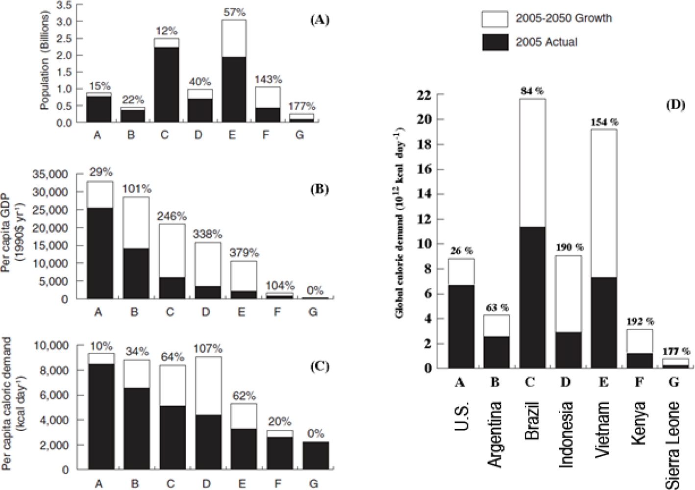
As demonstrated [3], on a global scale, per capita food demand is closely related to per capita GDP (Figure 1). For example, people in the richest countries (group A—example US) consume roughly 8,000 kcal·day−1 compared to an average consumption of 4,000 kcal·day−1 for people in group C and D (Brazil and Indonesia, respectively). Taking this into account and assuming that the Gross Domestic Product (GDP) and global population will continue to increase in the future, the past trend of strongly increasing food demand is expected to last for 3–4 decades. Tilman et al. (2011) [3] project that per capita demand for crops (caloric and/or protein) will double between 2005 and 2050. The strongest increases (in absolute values) are predicted within economic groups C to E (Figure 2(D)). The predictions are based on forecasts of per capita real income in 2050 (Figure 2(B)) and by a projected 2.3 billion person increase in global population (Figure 2(A)). The predictions within each economic group also take into account shifts in food demand and quality with increased per capita real GDP and assume that GDP increases by 2.5% annually between 2000 and 2050.
Based on this and other forecasts, most agronomists and international food organizations, such as the FAO, agree that food production must grow substantially for meeting the world’s future food security and sustainability needs. At the same time, agriculture’s environmental footprint must shrink dramatically (Figure 3) [2,16,17]. Hence, in the coming decades, a crucial challenge for humanity will be meeting future food demands without undermining further the integrity of the Earth’s environmental systems [4]. The necessary transformation will have to take place in times of climate change, adding supplementary difficulties [18]. For example, it is expected that temperature and precipitation patterns will change in the next decades, with more frequent extreme meteorological conditions [17,19]. This transition should be monitored at various temporal and spatial scales.
2.2. Environmental Impacts of Agriculture and Future Pathways for Increasing Agricultural Production
Agriculture and natural resources are both under strong pressure. The main drivers are population growth, increasing consumption of calorie- and meat-intensive diets and an increasing use of cropland for bioenergy production [2,20–22]. The negative impacts of current agriculture are manifold and can be related to either agricultural expansion or intensification [2,3]:
biodiversity is threatened by land clearing and habitat fragmentation [23];
greenhouse gas (GHG) emissions from land clearing, crop production and fertilization contribute already to 1/3 of global GHG emissions [24];
global nitrogen and phosphorus cycles have been disrupted, with impacts on water quality, aquatic ecosystems and marine fisheries [25,26];
freshwater resources are depleted, as nearly 80 percent of freshwater currently used by humans is for irrigation [27–29].
The most harmful environmental impacts of agriculture are shown in the lower part of Figure 3. The ‘−’ sign indicates that a reduction of the respective impact is necessary.
The environmental impacts of doubling global crop production will depend on how increased production is achieved [2,3]. Production could be increased by agricultural extensification or intensification. Extensification implies clearing additional land for crop production. Intensification, on the other hand, achieves higher yields through increased inputs, improved agronomic practices (e.g., drop irrigation), improved crop varieties and other innovations. Papers [30–33] demonstrate how remote sensing can contribute to the mapping of land under agricultural production. The review paper of Rembold et al. (this issue) [34] provides an overview of remote sensing techniques for yield mapping. The reconstruction of past land use systems is exemplified in [35,36].
According to [3], the ‘land sparing trajectory’ (i.e., intensification) is the preferred solution, as closing the yield gap would minimize both land clearing and greenhouse gas (GHG) emissions, compared to a continuation of current practices (‘past trend trajectory’). The yield gap is here defined as the difference between realized productivity and the best that can be achieved using current genetic material. The land sparing trajectory could meet the 2050 projected global crop demand, while clearing “only” 0.2 billion ha of land globally (compared to 1.0 billion ha) and producing global GHG emissions of “just” 1 Gt·yr−1 (instead of 3 Gt·yr−1).
Foley et al. (2011) [2] demonstrate that tremendous progress could be made by halting agricultural expansion, closing yield gaps on underperforming lands, increasing cropping efficiency, shifting diets and reducing waste. Together, these five strategies could double food production, while greatly reducing the environmental impacts of agriculture. Similar conclusions are drawn by Godfray et al. (2010) [17], who promote a “multifaceted and linked global strategy” to ensure sustainable and equitable food security.
Current yield gaps were quantified by [3,4], amongst others. They demonstrate that current yield differences among nations are large (Figure 4). In 2005, for example, caloric yields (per ha) for Group A nations (e.g., USA) were 138% greater than for Group E (e.g., Vietnam) and 37% greater than for Groups B (e.g., Argentina), C (e.g., Brazil) and D (e.g., Indonesia). Compared to the poorest countries (e.g., Kenya and Sierra Leone, belonging to Groups F and G, respectively), yield gaps were even higher (e.g., 308%). This analysis—incorporating the effects of climate and soils on yields—suggests that agricultural intensification would greatly reduce these yield gaps, provide a more equitable food supply and greatly decrease the GHG emissions and species extinctions that otherwise would result from land clearing and agricultural expansion. The necessary transformation process has to be initiated, taking social and societal issues into account.
This view is also shared by Foley et al. (2011) [2]. Their analysis shows that many nations have a high potential for closing yield gaps (Figure 5(A)). In some countries, additional calories could be produced by allocating a higher fraction of the cropland to growing food crops (crops that are directly consumed by people) instead of using this land for animal feed, bioenergy crops and fibers, etc. (Figure 5(B)).
Strong differences exist in the use of cropland for crop production allocated to human food (Figure 5(C)). [2] find that, globally, only 62% of crop production is for human food, versus 35% to animal feed and 3% (with an increasing trend) for bioenergy and other industrial products. Whereas Africa and Asia allocate typically over 80% of their cropland to food crops, North America and Europe devote only about 40% to direct food production; in the upper Midwestern US, less than 25%. Although animal feed produces human food indirectly (e.g., meat and dairy products), efficiency is much less. The whole system is still very dynamic [30,37]. The paper of Udelhoven et al. (this issue) [38] exemplifies how remote sensing can be used to map the bioenergy potential of maize crops. Rangeland identification and monitoring is, for example, described in [39].
Mueller et al.[4] find that, globally, large production increases (45% to 70% for most crops) are possible from closing yield gaps to 100% of attainable yields (Figure 4). Required changes in management practices that are needed to close yield gaps vary considerably by region (Figure 6). At the same time, Mueller et al.[4] find that there are large opportunities to reduce the environmental impact of agriculture by eliminating nutrient overuse, while still allowing an approximately 30% increase in production of major cereals (e.g., maize, wheat and rice). They conclude that meeting the food security and sustainability challenges of the coming decades is possible, but will require considerable changes in nutrient and water management. The papers [14,15,36] of this issue illustrate how remote sensing can be used in pest, water and nitrogen management (see also [40–42]). Because of its strong link to crop status and yield potential, leaf area index (LAI) mapping is another valuable remote sensing contribution. The papers of Gowda et al. (this issue) [43], Vuolo et al. (this issue) [44] and Shen et al. (this issue) [45] illustrate this important application. Yield mapping for different crops is further exemplified in papers [30–32,34,46,47] of this issue.
2.3. Evidence-Based Decision Making
Of course, agricultural policies have to take into account many other aspects not discussed here (e.g., social and economic factors, international policies, strategic considerations). However, whatever decision is taken, it should be evidence-based (i.e., well-grounded and based on reliable information) [48]. Probably the best way for gaining unbiased information over large areas is through satellite-based remote sensing. For this reason, world-wide investments in this area are necessary. Monitoring systems are needed to inform policy makers and stakeholders about the state of the agricultural sector and the pathway that led to the current situation. Information is also critical for impact assessment. Together, this would facilitate risk reduction and would lead to optimized statistical analyses at a range of scales, enabling a timely and accurate national to sub-national agricultural statistical reporting. The papers of Zhang et al. (this issue) [37], Edlinger et al. (this issue) [36] and Atzberger & Rembold (this issue) [35] show how remote sensing can be used to map past conditions. This permits, for example, gaining evidence regarding the effects of (agricultural) policies on land use.
A timely, comprehensive, transparent, accurate and unbiased agricultural monitoring system also prevents excessive market speculation and resulting price spikes [49]. As the poorest people are generally the most affected by rising food prices, the social component of an effective monitoring system becomes visible. We all should feel ashamed that still one billion people are chronically malnourished (UN, 2001) [50]. The paper of Becker-Reshef et al. (2009) [51] details the Group on Earth Observations (GEO) initiative aiming to support the building of a global monitoring capacity for food security.
Remote sensing data can greatly contribute to the monitoring task by providing timely, synoptic, cost efficient and repetitive information about the status of the Earth’s surface [52]. The data recorded by current remote sensing satellites can be used to assess the two components of crop production [53]: yield [30–32,34,46,54] and acreage [10,37]. In addition, crop phenological information [12,55], stress situations [14,34,56] and disturbances [13,57] can be detected. Amongst other things, the retrieved information permits decision makers to better anticipate the effects of (disastrous) climatic events (predicted to increase in strength and frequency) and to get an objective and unbiased spatial picture over large areas (for risk assessment). By putting the current situation in an historical context, an agricultural monitoring system permits better understanding of the possible effects of climate change (for preparedness and mitigation) and identification of areas with the highest yield potential. As discussed above, closing this yield gap is one of the top priorities in the upcoming decades [2,3]. With upcoming new sensors, such as the European Sentinel and Proba-V satellites, data provision will be further facilitated. However, sensor inter-calibration is still an important issue, as illustrated in Yin et al. (this issue) [58] and Meroni et al.[59].
3. Existing Operational Large-Scale Agricultural Monitoring Systems
Agriculture monitoring is not a new concern. In fact, the basics of geometry and land surveying were developed in ancient Egypt [60]. The aim was assessing cultivated areas affected by water level fluctuations of the River Nile, with the purposes of taxation and for preventing famine. Today, a regional to global agricultural intelligence is needed to respond to various societal needs. For example, national and international agricultural policies, global agricultural trade and organizations dealing with food security issues heavily depend on reliable and timely crop production information [6].
Agricultural monitoring systems should be able to provide timely information on crop production, status and yield in a standardized and regular manner at the (sub)regional to the national level. Estimates should be provided as early as possible during the growing season(s) and updated periodically through the season until harvest. Based on the information provided, stakeholders are enabled to take early decisions and identify geographically the areas with large variation in production and productivity. The system should provide homogeneous and interchangeable data sets with statistically valid precision and accuracy. Probably, only (satellite) remote sensing—combined with sophisticated modeling tools—can provide such information in a timely manner, over large areas, in sufficient spatial detail and with reasonable costs [61].
As outlined in a recent review by Becker-Reshef et al.[6], preliminary research and development on satellite monitoring of agriculture started with the Landsat-1 system (ERTS) in the early 1970s. According to the authors, unanticipated severe wheat shortages in Russia drew attention to the importance of timely and accurate prediction of world food supplies. As a result, in 1974, the USDA, together with NASA and NOAA, initiated the Large Area Crop Inventory Experiment (LACIE) [62,63]. The goal of this experiment was to improve domestic and international crop forecasting methods [64]. With enhancements that became available from the NOAA AVHRR sensor (Advanced Very High Resolution Radiometer), allowing for daily global monitoring, the AgRISTARS (Agriculture and Resource Inventory Surveys Through Aerospace Remote Sensing) program was initiated in the early 1980s [6]. Through the research conducted in these NASA-USDA joint programs, the considerable potential for use of remotely sensed information for monitoring and management of agricultural lands was identified. One of the most recent efforts that NASA and the USDA Foreign Agricultural Service (FAS) have initiated is the Global Agricultural Monitoring (GLAM) Project [6,51]. The GLAM project focuses on applying data from NASA’s MODIS (Moderate Resolution Imaging Spectroradiometer) instrument to feed FAS Decision Support System (DSS) needs [65].
Besides the USDA (FAS) GLAM system, there are currently several other regional to global operational agricultural monitoring systems providing critical agricultural information at a range of scales [6,53,66]:
the USAID Famine Early Warning System (FEWS-NET) [67]
the UN Food and Agriculture Organization (FAO) Global Information and Early Warning System (GIEWS) [68];
JRC’s Monitoring Agricultural ResourceS (MARS) action of the European Commission in Ispra (Italy) with two different topics: agricultural production estimates of EU countries (Agri4Cast [69]) and food security assessments in food insecure countries (FoodSec) [70];
the European Union Global Monitoring of Food Security (GMFS) program [71]
the Crop Watch Program at the Institute of Remote Sensing Applications (IRSA) of the Chinese Academy of Sciences (CAS) [72].
However, the USDA FAS with its GLAM system is currently the only provider of regular, timely, objective crop production forecasts at a global scale. This unique capability is in part afforded by the USDA’s partnership with NASA, providing global coverage of Earth observation data, as well as analysis tools for crop condition monitoring and production assessment at the global scale [6]. The GLAM project is also playing a leadership role in the Group on Earth Observations (GEO) agricultural monitoring component AG-07-03. GEO itself is part of GEOSS (Global Earth Observation System of Systems), providing decision-support tools to a wide variety of users. Recently, the GEOGLAM initiative was created integrating GLAM into GEOSS [73].
At high revisit frequency, the Earth’s land surface can currently only be covered by coarse/medium resolution sensors, such as MODIS. Consequently, a monitoring system must heavily rely on time series provided by such sensors. With the upcoming Sentinel’s 2 and 3 (to be launched by the end of 2014) and Proba-V sensors [74] a new era of Earth observation will be entered. First of all, data availability at coarse/medium resolution will increase (e.g., Sentinel 3 providing data at 300 m ground sample distance (GSD) and Proba-V at 100 m). Even more exciting, Sentinel-2 will provide 10–30 m data at five-day revisit intervals. The Venus sensor will be launched in 2014 with 12 spectral bands (5 m ground resolution) and a two-day’s revisiting time. The hyperspectral HyspIRI will be launched between 2013 and 2016 with a spectral resolution of 10 nm, 19-day’s revisiting time and a spatial resolution of 60 m. The Landsat data continuity mission (LDCM) is planned for launch very soon. The free data will also include two thermal bands for energy balance calculations. Together, this will open new opportunities for crop monitoring. The community should prepare now for this new data sources. Urgently needed are, for example, robust pre-processing and filtering chains [75]. Furthermore, inter-calibration issues must be solved [58].
4. Remote Sensing of Agricultural Resources
Already in the early 80s, it was shown by Tucker and co-workers that green vegetation can be monitored through its spectral reflectance properties [76,77]. Today, a large range of satellite sensors provide us regularly with data covering a wide spectral range (from optical through microwave). Data are acquired from various orbits and in different spatial and temporal resolutions. For deriving the sought information, a large number of spectral analysis tools have been developed. Besides the spectral signature, useful information can also be retrieved by analyzing the temporal signature (e.g., [11,52,78–82]) and directional reflectance properties of vegetation (e.g., [83–86]). Further useful information can also be retrieved from the spatial arrangement of the pixels, i.e., the texture of the image, even at coarse resolution [87].
4.1. Biomass and Yield
In the early 80s, Tucker and co-workers [76,77] found that arithmetic combinations of vegetation reflectances in the red and near infrared (so called “vegetation indices” or VI) are particularly useful for vegetation characterization. For example, the well known NDVI (Normalized Difference Vegetation Index) was already proposed in 1978 by Deering. The index became, subsequently, the most popular indicator for studying vegetation health and crop production. The success of the NDVI stems from its close relation to the canopy Leaf Area Index (LAI) and fAPAR (fraction of Absorbed Photosynthetically Active Radiation) [88,89]. Due to its almost linear relation with fAPAR, the NDVI can be readily used as an indirect measure of primary productivity. In Rembold et al. (this issue) [34], a comprehensive overview is provided regarding biomass and yield mapping approaches. Different methods are discussed, ranging from simple regression equations, to the use of more complex crop growth models [90]. For this reason, the present section focuses only on the so-called ‘yield correlation masking’. Strong reference is made to the excellent publication of Kastens et al.[7]. It has also to be noted that time integration analysis generally increases the prediction accuracy, as, for example, presented in this special issue ([32,46]).
One obstacle to successful modeling and prediction of crop yields using remotely sensed imagery is the identification of image masks [7]. Image masking involves restricting an analysis to a subset of a region’s pixels, rather than using all of the pixels in the scene. Cropland masking, where all sufficiently cropped pixels are included in the mask regardless of crop type, has been shown to generally improve crop yield forecasting ability. [91], for example, used three years of AVHRR NDVI imagery to assess spring wheat yields in North and South Dakota in the US. They concluded that the most promising way to improve the use of AVHRR NDVI for estimating crop yields at regional scales would be to use better crop masks. This was also confirmed by [92]. They used a 10-year, bi-weekly AVHRR data set to forecast corn yields in the US state of Iowa. They found that the most accurate forecasts of crop yield were made using accumulated NDVI and a cropland mask. Similarly, [93] found that application of cropland masks improved relationships between NDVI and final yield in four Mediterranean countries. Vancutsem et al. (this issue) [94] illustrate the difficulties encountered when harmonizing and combining existing land cover maps.
For crop yield forecasting, the ideal approach would be to use crop-specific masks. This would allow one to consider only NDVI information pertaining to the crop of interest. However, when such masking is applied to multiple years of imagery, several difficulties are encountered [6]. A major problem relates to the widespread practice of crop rotation. In areas with crop rotation, a single crop-specific mask would not be appropriate. Instead, year-specific masks are needed. Identifying a particular crop in the year to be forecasted presents even greater difficulties, as only incomplete growing season NDVI information is available. This is especially true early in the season, when the crop has low biomass and does not produce a large NDVI response. Moreover, with medium/coarse resolution (about 25–100 ha/pixel) imagery, identifying mono-cropped pixels is not always feasible. This is particularly true in low-producing regions and in regions with sparse crop distribution. The unmixing of medium/coarse resolution data for a specific crop is challenging, as demonstrated by Atzberger and Rembold (this issue) [35]. The combined use of high resolution and medium resolution data for crop area estimation is further demonstrated by Zhang et al. (this issue) [37].
A more feasible alternative to crop-specific masking is cropland masking, which refers to using pixels dominated by ‘arable land’. The above mentioned studies [91–93] used this approach. Cropland masks usually are derived from existing land use/land cover maps. If relatively small amounts of land in a study area have been taken out of or put into agricultural crop production during a study period, a single mask can be obtained and applied to all years of data. Albeit simpler to realize compared to crop-specific masking (i.e., one mask per crop type and year), it has to be considered that all agricultural crops are now lumped in the general class of ‘cropland’. Thus, crop-specific growth patterns are neglected.
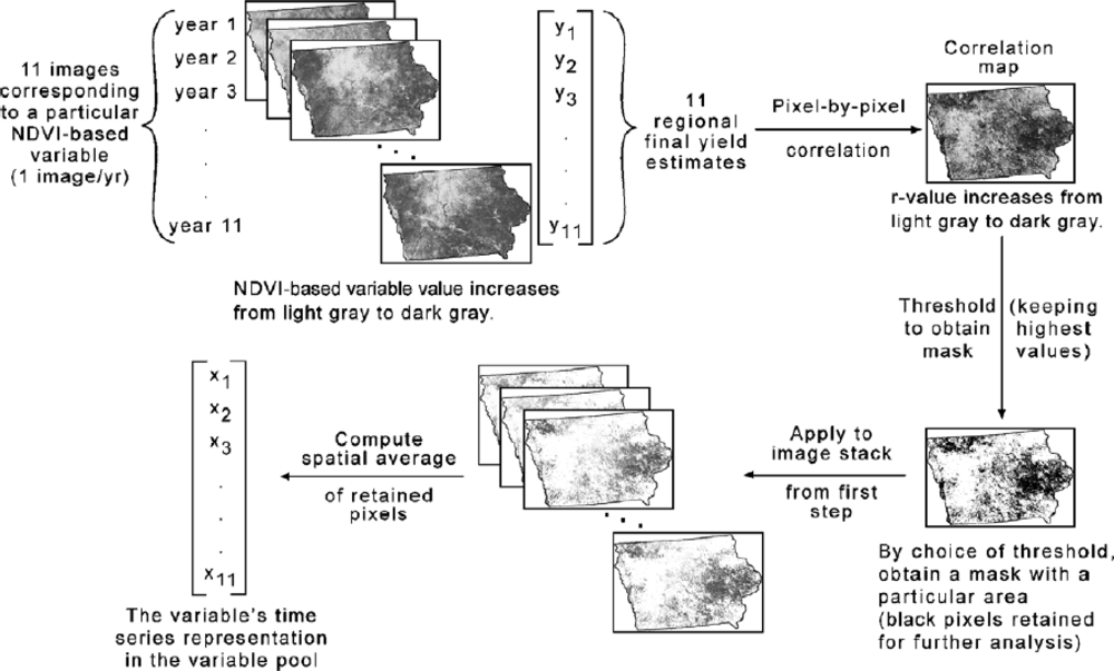
To overcome the shortcomings related to cropland masking and crop-specific masking, Kastens et al.[7] proposed a new masking technique, called yield-correlation masking. The main idea behind this concept is that all vegetation in a region integrates the season’s cumulative growing conditions in some fashion. The vegetation response to growing conditions may even be more indicative of a crop’s yield potential than the crop itself. Hence, in the yield-masking approach, all pixels are considered for use in crop yield prediction. In practical terms, yield-correlation masking generates a unique mask for each NDVI variable and each pair of crop “x” region. The technique is initiated by correlating each of the historical, pixel-level NDVI variable values with the region’s final yield history. The highest correlating pixels are retained for further processing and evaluation of the variable at hand. Figure 7 shows a diagram outlining this process for a single NDVI layer.
Though computationally more intensive, the yield-correlation masking technique overcomes the major problems afflicting crop-specific masking and cropland masking [6]. Unlike these approaches, yield-correlation masking readily can be applied to low-producing regions and regions possessing sparse crop distribution. Also, since yield-correlation masks are not constrained to include pixels dominated by cropland, they are not necessarily hindered by the weak and insensitive NDVI responses exhibited by crops early in their respective growing seasons. Furthermore, once the issue of identifying optimal mask size (i.e., determining how many pixels should be included in the masks) is addressed, the entire masking/modeling procedure becomes completely automated. Another important appeal of yield-correlation masking is that no land cover map is required to implement the procedure, while the procedure results in forecasts of comparable accuracy to those obtained when using cropland masking or crop-specific masks [7]. The procedure only requires an adequate time series of imagery and a corresponding record of the region’s crop yields. Problems regarding this approach can be expected when the land cover/land use of the selected yield proxies changes. The combined use of data sets from different sensors remains difficult, given the observed large discrepancies described, for example, in Yin et al. (this issue) [58].
4.2. Vegetation Vigor and (Drought) Stress Monitoring
In agricultural monitoring, timely and spatialized information about general growing conditions of the vegetated land is of high importance. For this reason, the use of satellite imagery for plant stress monitoring became an important remote sensing application [95,96]. In these ‘early warning’ approaches, the actual VI (at time t) is compared against the corresponding long-term-average to indicate if the actual vegetation conditions are favorable (VI higher than average) or worse (VI lower than average) compared to the ‘usual’ situation. Such relatively simple approaches are still widely used in the food security context. More details are provided in Rembold et al. (this issue) [34].
For monitoring vegetation stress (in particular, drought) simple VI-based approaches are often not sufficient. The main drawbacks relate to the fact that they often rely only on one parameter (the observed VI) and do not consider the persistence of the stress periods (Balint et al., 2011) [9]. Hence, in the absence of easy-to-use monitoring tools and methodologies, often rudimentary methodologies are used, like the annual rainfall amount. However, sometimes even a few weeks of unfavorable climate conditions induce already serious plant stress. Hence, simple rainfall anomalies are not well suited for real-time monitoring purposes.
A suitable drought index should combine information about precipitation, temperature and soil moisture strength and persistence. Such an index was, for example, conceived by [9] and termed Combined Drought Index (CDI).
In the CDI approach, drought (or vegetation stress) is conceived as a combination of:
a precipitation component, which considers rainfall deficits and persistence of dryness;
a temperature component, which considers temperature excesses and persistence of high temperatures;
a soil moisture component, which considers soil moisture deficits and persistence of dry soil conditions.
Because of the limited availability of soil moisture observations at 1-km resolution or better, [9] propose to approximate the soil moisture component by NDVI deficits and deficit persistence. The three individual drought indices PDI (Precipitation Drought Index), TDI (Temperature Drought Index) and VDI (Vegetation Drought Index—as a substitute for the Soil Moisture Drought Index)—are combined as a weighted sum to yield the CDI (Equation 1):
By definition, CDI = 1.0 represents average weather conditions. If the CDI is greater than 1.0, it represents wetter than average; if it is below 1.0, it represents dryer than average conditions. Drought severity categories may be fitted to geographic locations and/or plant types. Another advantage of this index is that it allows for flexible weightings (wPDI, wTDI and wVDI) of the three individual components.
Maps of CDI for the 2010–2011 drought period in the Greater Horn of Africa (GHA) are shown in Figure 8(A). A temporal profile is shown in Figure 8(B) for Belet Weyne in Somalia together with previous strong drought periods in 2000 and 2006. In the future, such information should help international organizations, such as the UN and FAO, to declare famine early enough to prevent human losses. Regarding the 2010–2011 drought, famine was declared by the UN only in July 2011.
4.3. Crop Phenological Development
The phenological dynamics of terrestrial ecosystems reflect the response of the Earth’s biosphere to inter- and intra-annual dynamics of the Earth’s climate and hydrologic regimes [98]. Remotely sensed satellite data possess significant potential for monitoring vegetation dynamics, due to their synoptic coverage and frequent temporal sampling. This enables the monitoring of simple phenological events, such as the start and peak of vegetation growth, both in natural ecosystems and in agricultural landscapes (Figure 9).
Besides being a proxy of a crop’s phenological development (sometimes closely related to crop yield—for example, cool summers may result in delayed heading and, thus, decreased yields), the temporal signature of vegetated surfaces is also useful for distinguishing land-cover types and for mapping land-use change [11,78,79,82]. This “double use” makes phenological metrics very interesting within agricultural monitoring systems. Croplands, for example, present a more complex phenology than natural land cover, due to their many peaks resulting from multiple crops planted sequentially within a growing season [10,99,100]. Additionally, the uniform cover of green leaves in an agricultural field creates very high observed greenness, especially as compared to the bare soils left after harvest. Consequently, several studies have identified land cover based on specific properties of the observed green leaf phenology, such as start of season, dry season minimums and amplitude of maximums (e.g., [10,78,98,101,102]). Other studies analyze the detected phenological indicators with respect to climate variables [103] and/or run trend analysis [104].
To determine the timing of vegetation green-up and senescence from remotely sensed VI time series, a number of different approaches have been developed. Following Beck et al., (2006) [105], the different methods can be grouped in two categories:
methods estimating the timing of single phenological events [106–108];
methods modeling the entire time series using a mathematical function [109,110].
Approaches belonging to the first group include:
the detection of the largest NDVI increase between two consecutive observations [112];
and backward-looking moving averages [106].
More recently, [98] used the rate of change in the curvature of a locally fitted logistic model to identify phenological transition dates. Specifically, transition dates correspond to the times at which the rate of change in curvature in the VI data exhibits local minima or maxima. These dates indicate when the annual cycle transitions from one approximately linear stage to another.
Methods for analyzing entire time series include:
Modeling VI time series as such has the advantage of conserving a maximum amount of information in the VI data, while reducing the dimensionality of the data [117]. Therefore, in addition to the phenological dates, other parameters can be estimated from the models output [105]. However, such methods are difficult to apply for large regions and generally do not account for ecosystems characterized by multiple growth cycles (e.g., double- or triple-cropping systems, semiarid systems with multiple rainy seasons, etc.). This was demonstrated, for example, recently by Atkinson et al.[99] over India.
The traditional Fourier transform, for example, expects periodicity in the data not always given (e.g., in the case of land use change). Additionally, application of Fourier transforms often reveals spurious oscillations [118]. This happens frequently when many harmonics have to be combined for fitting non-trivial temporal patterns (e.g., related to double/triple cropping).
Non-stationary data with irregular temporal shapes is better handled by the wavelet transform [10]. In agricultural applications, a wavelet-smoothed time series can be used to identify the start of the growing season and the time of harvest with relatively low errors (±2 weeks [12]). Wavelet analysis is capable of handling the range of agricultural patterns that occur through time, as well as the spatial heterogeneity of fields that result from precipitation and management decisions, because the transform is localized in time and frequency.
Curve fitting using pre-defined functions (e.g., double logistic) is another approach modeling the entire time series [105]. A fitted curve simplifies the parameterization necessary for identification of metrics, such as start of season. In addition, data gaps are easily handled. A drawback of curve-fitting approaches is that a priori information is necessary to inform the algorithm about the number of cropping seasons within a 12-month period and the probable location of vegetation peaks [117]. A large number of additional temporal features can be extracted using software like TimeStats (Udelhoven, 2011) [119].
4.4. Crop Acreage Estimation and Cropland Mapping
Cropland areas are often characterized by a diverse mosaic of LULC types that change over various spatial and temporal scales in response to different management practices and agricultural policies (e.g., [35,120–123]). As a result, detailed regional-scale cropping patterns need to be mapped on a repetitive basis [11,124]. Such information is also necessary to better understand the role and response of regional cropping practices in relation to various environmental issues (e.g., climate change, groundwater depletion, soil erosion) that potentially threaten the long-term sustainability of major agricultural producing areas [10]. Of course, for each growing season, the acreage of the different crops must be known for accurate production estimates [69,125–127]. The excellent work of Wardlow et al. (2007) [11] provides a valuable discussion of different approaches. Below is a summary of this work.
Remotely sensed data from satellite-based sensors have proven useful for large-area LULC characterization due to their synoptic and repeat coverage. Considerable progress has been made classifying LULC patterns using multispectral, high resolution Landsat TM data as a primary input [128]. Advances in LULC classification have also been made at national to global scales using multi-temporal, coarse resolution data (1 and 8 km) from NOAA-AVHRR [129]. The high temporal resolution of satellite time-series data allows land cover types to be discriminated based on their unique phenological (seasonal) characteristics [82,130]. However, few of these mapping efforts have classified detailed, crop-related LULC patterns, particularly at the annual time step required to reflect common agricultural LULC changes [11]. On the contrary, existing LULC maps often reveal strong differences, making harmonization attempts necessary [94].
The development of a regional-scale crop mapping and monitoring protocol is challenging, because it requires remotely sensed data that have wide geographic coverage, high temporal resolution, adequate spatial resolution relative to the grain of the landscape (i.e., typical field size) and minimal cost. Remotely sensed data from traditional sources, such as Landsat and AVHRR, have some of these characteristics, but are limited for such a protocol, due to their spatial resolution, temporal resolution, availability and/or cost. Compared to (1–8 km) AVHRR data, MODIS offers an opportunity for detailed, large-area LULC characterization by providing global coverage with daily revisit frequency and intermediate spatial resolution (250 m) [52]. The dataset is available at no cost, including 16-day composites of NDVI and enhanced vegetation index (EVI) updated every eight days. Several studies have already successfully demonstrated the potential of these data for detailed LULC characterization in an agricultural setting [11,79].
Wardlow et al.[11], for example, concluded that MODIS time-series at 250 m ground resolution had sufficient temporal and radiometric resolution to discriminate major crop types and crop-related land use practices in Kansas, US. For each crop, a unique multi-temporal VI profile was detected that was consistent with the known crop phenology. Most crop classes were separable at some point during the growing season based on their phenology-driven differences expressed in the VI data. Even regional intra-class variations were detected, reflecting the climate and planting date gradient in the study area. They also found that MODIS’s 250 m spatial resolution was an appropriate scale at which to map the general cropping patterns of the US Central Great Plains. For coffee monitoring, Bernardes et al. (this issue) [30] found MODIS data also very suitable. MODIS data was also found promising for crop area extraction by Zhang et al. (this issue) [37].
4.5. Disturbances and Land Use/Land Cover Changes
Monitoring the time and location of land-cover changes is important for establishing links between policy decisions, regulatory actions and subsequent land-use activities, as outlined by Galford et al. (2008) [10]. Regional shifts in land-cover and land-use have numerous consequences relevant to both environment and agriculture, including changes in nutrient cycles, water quality and biodiversity. Determining the physical and temporal patterns of agricultural extensification or expansion and intensification is the first step in understanding their implications, for example, for long-term crop production and environmental, agricultural and economic sustainability [10].
Traditionally, either pre- or post-classification change detection methods were applied to monitor land-cover changes. Both approaches reveal serious drawbacks (reviewed in [131]). For example, according to [10], factors that limit the application of post-classification change detection techniques can include cost, consistency and propagation of errors [132]. Drawbacks of pre-classification techniques, such as Principle Component Analysis (PCA) [133] or Change Vector Analysis (CVA) [134], relate in large parts to phenology-induced errors [132]. For example, plants undergo intra-annual cycles related to their growth and development patterns. During different stages of vegetation growth, plant structures and associated pigment assemblages can vary significantly. Thus, the same vegetation type can appear significantly different and different types similar, at various stages during intra-annual growth cycles. A fine-tuning of change thresholds is thus necessary to separate ‘real’ changes from ‘natural’ variations. Besides these problems, Foody (2010) [135] points out the importance of ground truthing. The papers [33,35–37] of this special issue provide examples on how to use remote sensing data for reconstructing past land use patterns at the landscape level.
To move towards threshold-independent change detection, trajectory-based change detection methods have been proposed taking implicitly the temporal signature into account [136–139]. As outlined by [13], these supervised approaches require the definition of the change trajectory specific for the type of change to be detected and the spectral data to be analyzed. The trajectory-based change detection method thus only works well if the observed spectral trajectory matches one of the hypothesized trajectories.
As traditional change detection methods are often not capable of detecting land cover changes within a time series that are heavily influenced by seasonal climatic variations, Verbesselt et al. (2010) [13] developed a generic change detection approach, labeled BFAST (Breaks For Additive Seasonal and Trend). BFAST integrates the decomposition of a time series into trend, seasonal and remainder components with methods for detecting change within the time series (Figure 10). BFAST iteratively estimates the time and number of changes and characterizes change by its magnitude and direction. Detecting changes within the trend and seasonal components of a time series enables the classification of different types of changes. For example, changes occurring in the trend component often indicate disturbances (e.g., fires, insect attacks), while changes occurring in the seasonal component indicate phenological changes (e.g., change in land cover type) [13].
The use of MODIS data within disturbance approaches, such as BFAST, is particularly attractive, due to the cost-free data and the very low cost associated with data processing. These advantages are in sharp contrast to the traditional Landsat data-based approaches that are comparatively data and computationally expensive. The increased temporal resolution of the MODIS NDVI 250 m data has a significant advantage over traditional Landsat data for both capturing the actual timing of the change event and the subsequent monitoring of the recovery to the next steady state [132].
4.6. Noise-Removal
The previous five sub-sections outlined some important applications of medium to coarse resolution imagery for agricultural applications. The integration of time series of vegetation indices, such as NDVI or Enhanced Vegetation Index (EVI), in various modeling frameworks is nowadays facilitated by readily available and standardized (in time and space) products [75]. Such global composites have a high potential for continuous and real-time updating. However, despite the continuous effort for making these products globally available in near real-time (for example, from the online data pool at NASA LP DAAC LP DAAC: Land Processes Distributed Active Archive Center), various processing steps are still required before complete and efficient integration in any modeling framework is possible [75]. For instance, gap filling and data smoothing are routine operations that are not yet automated. Smoothing and gap-filling are, however, extremely important pre-processing steps. Even carefully (atmospherically and radiometrically) corrected VI data sets (e.g., from MODIS) still contain substantial amounts of noise [139] (Figure 11). The various noise components are related to aerosols, to undetected (sub-pixel) clouds, as well as to BRDF effects [140]. Data gaps result from prolonged periods of permanent cloud cover. Thus, noise reduction is essential before the ‘true’ temporal evolution of the measured VI can be extracted from the satellite data for deriving added-value products.
The simplest method for creating a smoothed time series is to use multi-point smoothing functions, such as moving averages or polynomial filters [119,141,142]. Other curve-fitting methods rely on a harmonic curve-fit to the annual average phenology to characterize inter-annual variability of a time series [102,143]. A sigmoid curve-fitting algorithm can be applied to a time series of a single year [98,105,144]. However, such pre-defined functions utilize a priori knowledge of the system's seasonality in order to detect the phenological peaks (i.e., the algorithm must be informed with expectation for when to find the phenological peak and how many peaks are expected during a given year) [117]. All of these methods have proven powerful in the systems they have been tested in, but generally fail in the case of complicated cropping patterns [10].
According to Sakamoto et al. (2005) [12], wavelet-based approaches are interesting alternatives, as they provide a more flexible fitting of the observations compared, for example, to Fourier-based approaches. With wavelets, it is feasible to identify the timing of events in the presence of noise. The wavelet transform retains time components when transforming time-series data and, so, can reproduce seasonal changes of vegetation without losing the temporal characteristics. In contrast, the trigonometric functions used in the Fourier transform (e.g., [114]) are not localized in the time domain, and therefore, the time component of the input data is averaged after the transforming process [12].
However, application of the wavelet filter can create distortion around the edges of the VI time series [12]. To avoid this problem, it is possible to allow for spin-up or conditioning of the wavelet. However, these workarounds come with additional (computational) costs. Another drawback of wavelets is that they are very sensitive to small maximums in portions of the time series, where the VI range is low [10]. The wavelet response to these small local maximums (slightly) amplifies small real peaks, thereby creating false peaks in phenology.
In a recent comparative study involving a number of commonly used filters, it was shown that the ‘Whittaker smoother’ (based on penalized splines) provides robust results for different noise levels and different cropping patterns (e.g., single vs. double cropping) [99]. The Whittaker smoother is based on penalized least squares. It fits a discrete series to discrete data and penalizes the roughness of the smooth curve using a single (continuous) parameter (λ: the smoothing parameter) (Figure 12(A)). In this way, it balances reliability of the data and roughness of the fitted data [144]. The filter can easily handle weights (i.e., MODIS QA flags) and inter/extrapolates automatically if data points are missing. Further details are given in [99,145,146]. A user-friendly GUI for downloading MODIS time series smoothed with the Whittaker filter is available at [147]. More detailed information regarding this MODIS tool can be found in Vuolo et al. (2012) [75]. The filter is also suitable for smoothing spectral signatures, as exemplified in (Figure 12(B)).
5. Conclusions and Recommendations
The review demonstrates the strong role remote sensing plays within the agricultural sector. The remotely provided information is urgently needed for various decision makers. Requests for objective information will increase in the future, as a result of the expected changes in the agricultural sector (e.g., meeting food requirements and environmental restrictions). For example, for most crops, large production increases (between 45 and 70%) are possible from closing yield gaps to 100% of attainable yields [4]. Remotely sensed information can help with identifying yield gaps and monitoring related agricultural practices. Using ‘yield-correlation masking’, this would even be possible without detailed crop masks, provided enough (historical) yield data is available. In parallel, environmentally sensitive areas could be identified for protective purposes. The detection of phenological indicators not only helps with identifying different land covers and crops (and crop growing conditions), but at the same time, provides evidence for ongoing global/climate change. With appropriate pre-processing of time series (gap filling and smoothing), phenological indicators, such as start of the growing season, can probably be estimated with accuracies of ±7–10 days. Vegetation anomalies related to local meteorological conditions (e.g., droughts) can be readily detected from space and combined with other data sources to indicate stress affected regions. This information is not only important for organizations dealing with food security, but can also helps with identifying a region’s vulnerability to (drought) stress. Finally, the detection and monitoring of (permanent) land-cover changes is, for example, important for establishing links between policy decisions, regulatory actions and subsequent land-use activities [10]. The challenge will be to integrate the above mentioned indicators so that complementary information can be derived. Although the described examples were mostly based on globally available (medium to coarse resolution) data sets, it is clear that additional information at high spatial resolution is available and should be integrated (plus ground sensors) (see for example [14,15,38,43–45,47] in this special issue). Thus, besides investments in the agricultural sector, the related monitoring components should be strengthened. Elements of the necessary monitoring component exist, but should be further integrated and consolidated.
Similar to the objectives of the GEOGLAM initiative [73], the following recommendations can be drawn from the review:
Agriculture depends strongly on the timeliness of the provided information. Information is worth little if it comes (too) late. Thus, the issue of timeliness should be dealt with in all developments;
Product developers have only limited access to ground truth information to evaluate their products under various environmental settings. International efforts are needed to establish such networks of validation sites. This also requires substantial funding by space agencies and/or environmental institutions. Interesting attempts are, for example, GeoWiki [148]) and JECAM [149];
Space agencies and sensor developers spend huge amounts of money for precise radiometric calibration of the deployed instruments. However, these efforts have little positive effect unless the much stronger radiometric distortions introduced by the atmosphere are removed. Operational implementations of precise atmospheric correction algorithms are mandatory. Instead of relying on (aerosol) climatologies, the algorithms should be fed with local atmospheric properties (probably also derived from satellites);
In the future, multi-sensor studies will become frequent. Thus, sensor inter-calibration studies are urgently needed;
Access of data and derived products is sometimes still too complicated. Efforts are necessary to permit users to visualize (and possibly download) information products in a very simple way (such as realized in Google Earth);
Approaches are still very scattered and not always implemented in operational processing chains. Funding organizations should facilitate international cooperation, while limiting administrative burdens;
For potential users, the wide variety of products can be confusing. Efforts are necessary to clearly explain the purpose (and limits) of a given product.
The tremendous increase in the use of Landsat data after 2008 has been demonstrated by Wulder et al. (2012) [150]. This was achieved by the decision of the US government and USGS to make the Landsat archive available at no costs (same for LDCM). ESA's current image distribution policy is a clear example of what should be avoided: tax payers spend billions for space and ground segments (for example, the MERIS sensor), but afterwards, hardly anyone uses the (excellent) data, because of an antiquated data distribution policy. Generally, data from national and international organizations should come free of costs. Such a decision would boost science and (commercial) remote sensing applications.
Acknowledgments
I would like to devote this article to my teachers and colleagues, Nadine Gobron and Gilbert Saint, who passed away too early. I am also grateful to a number of people who contributed directly and indirectly to this paper: Antonio Formaggio and Yosio Shimabokuro and their team from INPE (Sao Jose dos Campos) for shared drafting of a related research proposal for a Brazilian monitoring system; Felix Rembold (JRC Ispra) for discussing the original manuscript; Zoltan Balint, Peris Muchiri and SWALIM at FAO Somalia (Nairobi) for contributions regarding the CDI drought index; and Anja Klisch, Francesco Vuolo and Matteo Mattiuzzi (BOKU Vienna) for providing inputs related to vegetation phenology and the MODIS processing chain.
References
- Food and Agriculture Organization of the United Nations (FAO), Global Strategy to Improve Agricultural and Rural Statistics; Report No. 56719-GB; FAO: Rome, Italy, 2011.
- Foley, J.A.; Ramankutty, N.; Brauman, K.A.; Cassidy, E.S.; Gerber, J.S.; Johnston, M.; Mueller, N.D.; O’Connell, C.; Ray, D.K.; West, P.C.; et al. Solutions of a cultivated planet. Nature 2011, 478, 337–342. [Google Scholar]
- Tilman, D.; Balzer, C.; Hill, J.; Befort, B.L. Global food demand and the sustainable intensification of agriculture. Proc. Natl. Acad. Sci. USA 2011, 108, 20260–20264. [Google Scholar]
- Mueller, N.D.; Gerber, J.S.; Johnston, M.; Ray, D.K.; Ramankutty, N.; Foley, J.A. Closing yield gaps through nutrient and water management. Nature 2012. [Google Scholar] [CrossRef]
- Jonathan Foley. How to Feed Nine Million and Keep the Planet too, Available online: http://www.newsecuritybeat.org/2011/10/jon-foley-how-to-feed-nine-billion-and-keep-the-planet-too/#.USI9VKV303k (accessed on 18 February 2013).
- Becker-Reshef, I.; Justice, C.O.; Sullivan, M.; Vermote, E.F.; Tucker, C.; Anyamba, A.; Small, J.; Pak, E.; Masuoka, E.; Schmaltz, J.; et al. Monitoring global croplands with coarse resolution Earth observation: The Global Agriculture Monitoring (GLAM) project. Remote Sens 2010, 2, 1589–1609. [Google Scholar]
- Kastens, J.H.; Kastens, T.L.; Kastens, D.L.A.; Price, K.P.; Martinko, E.A.; Lee, R.-Y. Image masking for crop yield forecasting using AVHRR NDVI time series imagery. Remote Sens. Environ 2005, 99, 341–356. [Google Scholar]
- Zhang, P.; Anderson, B.; Tan, B.; Huang, D.; Myneni, R. Potential monitoring of crop production using a satellite-based Climate-Variability Impact Index. Agr. Forest Meteorol 2005, 132, 344–358. [Google Scholar]
- Balint, Z.; Mutua, F.M.; Muchiri, P. Drought Monitoring with the Combined Drought Index; FAO-SWALIM: Nairobi, Kenya, 2011. [Google Scholar]
- Galford, G.L.; Mustard, J.F.; Melillo, J.; Gendrin, A.; Cerri, C.C.; Cerri, C.E.P. Wavelet analysis of MODIS time series to detect expansion and intensification of row-crop agriculture in Brazil. Remote Sens. Environ 2008, 112, 576–587. [Google Scholar]
- Wardlow, B.D.; Egbert, S.L.; Kastens, J.H. Analysis of time-series MODIS 250 m vegetation index data for crop classification in the US Central Great Plains. Remote Sens. Environ 2007, 108, 290–310. [Google Scholar]
- Sakamoto, T.; Yokozawa, M.; Toritani, H.; Shibayama, M.; Ishitsuka, N.; Ohno, H. A crop phenology detection method using time-series MODIS data. Remote Sens. Environ 2005, 96, 366–374. [Google Scholar]
- Verbesselt, J.; Hyndman, R.; Newnham, G.; Culvenor, D. Detecting trend and seasonal changes in satellite image time series. Remote Sens. Environ 2010, 114, 106–115. [Google Scholar]
- Mirik, M.; Ansley, R.J.; Steddom, K.; Rush, C.M.; Michels, G.J.; Elliott, N.C. Analysis of high spectral and spatial resolution hyperspectral imagery for greenbug infestation in winter wheat using constrained energy minimization classifier. Remote Sens. 2013. in review. [Google Scholar]
- Zecha, C.W.; Link, J.; Claupein, W. Sensor platforms in precision farming: Categorization and research applications. Remote Sens. 2013. in review. [Google Scholar]
- The Royal Society. Reaping the Benefits: Science and the Sustainable Intensification of Global Agriculture, 2005. Available onoline: http://royalsociety.org/Reapingthebenefits (accessed on 18 February 2013).
- Godfray, H.C.J.; Beddington, J.R.; Crute, I.R.; Haddad, L.; Haddad, D.; et al. Food Security: The challenge of feeding 9 billion people. Science 2010, 327, 812–818. [Google Scholar]
- Jones, P.G.; Thornton, P.K. The potential impacts of climate change on maize production in Africa and Latin America in 2055. Global Environ. Change 2003, 13, 51–59. [Google Scholar]
- IPCC (Intergovernmental Panel on Climate Change), Climate Change 2007: Synthesis Report. Contribution of Working Groups I, II and III to the Fourth Assessment Report of the Intergovernmental Panel on Climate Change; IPCC: Geneva, Switzerland, 2007.
- The State of Food Insecurity in the World 2009: Economic Crises—Impacts and Lessons Learned; Food and Agriculture Organization of the United Nations (FAO): Rome, Italy, 2009.
- Hill, J.; Nelson, E.; Tilman, D.; Polasky, S.; Tiffany, D. Environmental, economic, and energetic costs and benefits of biodiesel and ethanol biofuels. Proc. Natl. Acad. Sci. USA 2006, 103, 1120–11210. [Google Scholar]
- Pelletier, N.; Tyedmers, P. Forecasting potential global environmental costs of livestock production 2000–2050. Proc. Natl. Acad. Sci. USA 2010, 107, 18371–18374. [Google Scholar]
- Dirzo, R.; Raven, P.H. Global state of biodiversity and loss. Annu. Rev. Environ. Resour 2003, 28, 137–167. [Google Scholar]
- Burney, J.A.; Davis, S.J.; Lobell, D.B. Greenhouse gas mitigation by agricultural intensification. Proc. Natl. Acad. Sci. USA 2010, 107, 12052–12057. [Google Scholar]
- Vitousek, P.M.; Aber, J.D.; Howarth, R.W.; Likens, G.E.; Matson, P.A.; Schindler, D.W.; Schlesinger, W.H.; Tilman, D.G. Human alteration of the global nitrogen cycle: Sources and consequences. Ecol. Appl 1997, 7, 737–750. [Google Scholar]
- Canfield, D.E.; Glazer, A.N.; Falkowski, P.G. The evolution and future of Earth’s nitrogen cycle. Science 2010, 330, 192–196. [Google Scholar]
- Thenkabail, P.S.; Biradar, C.M.; Noojipady, P.; Dheeravath, V.; Li, Y.; Velpuri, M.; Velpuri, M.; Reddy, G.P.O.; Cai, X.L.; Gumma, M.; et al. Global irrigated area map (GIAM), derived from remote sensing, for the end of the last millennium. Int. J. Remote Sens 2009, 30, 3679–3733. [Google Scholar]
- Thenkabail, P.S. Global croplands and their importance for water and food security in the twenty-first century: Towards an ever green revolution that combines a second green revolution with a blue revolution. Remote Sens 2010, 2, 2305–2231. [Google Scholar]
- Postel, S.; Daily, G.C.; Ehrlich, P.R. Human appropriation of renewable fresh water. Science 1996, 271, 785–788. [Google Scholar]
- Bernardes, T.; Moreira, M.A.; Adami, M.; Giarolla, A.; Rudorff, B.F.T. Monitoring biennial bearing effect on coffee yield using MODIS remote sensing imagery. Remote Sens 2012, 4, 2492–2509. [Google Scholar]
- Duveiller, G.; Lopez, R.; Baruth, B. Enhanced processing of low spatial resolution fAPAR time series for sugarcane yield forecasting and monitoring. Remote Sens. 2013. in review. [Google Scholar]
- Mulianga, B.; Begue, A.; Simoes, M.; Todoroff, P. Forecasting regional sugarcane yield based on time integral and spatial aggregation of MODIS NDVI. Remote Sens. 2013. in reivew. [Google Scholar]
- Guerriero, L.; Pierdicca, N.; Pulvirenti, L.; Ferrazzoli, P. Use of satellite radar bistatic measurements for crop monitoring: A simulation study. Remote Sens 2013, 5, 864–890. [Google Scholar]
- Rembold, F.; Atzberger, C.; Rojas, O.; Savin, I. Using low resolution satellite imagey for yield prediction and yield anomaly detection. Remote Sens. 2013. in review. [Google Scholar]
- Atzberger, C.; Rembold, F. Mapping the spatial distribution of winter crops at sub-pixel level using AVHRR NDVI time series and neural nets. Remote Sens. 2013. in review. [Google Scholar]
- Edlinger, J.; Conrad, C.; Lamers, J.; Khasankhanova, G.; Koellner, T. Reconstructing the spatio-temporal development of irrigated production systems in Uzbekistan using Landsat time series. Remote Sens 2012, 4, 3972–3994. [Google Scholar]
- Zhang, J.; Feng, L.; Yao, F. Crop area extraction by the integration of MODIS-EVI time series data and China’s high spatial resolution Environment Satellite (HJ-1) data. Remote Sens. 2013. in review. [Google Scholar]
- Udelhoven, T.; Delfosse, P.; Bossung, C.; Ronellenfitsch, F.; Mayer, F.; Schlerf, M.; Machwitz, M.; Hoffmann, L. Retrieving the bioenergy potential from maize crops using hyperspectral remote sensing. Remote Sens 2013, 5, 254–273. [Google Scholar]
- Röder, A.; Udelhoven, T.; del Barrio, G.; Tsiourlis, G.M. Trend analysis of Landsat-TM and -ETM+ imagery to monitor grazing impact in a rangeland ecosystem in Northern Greece. Remote Sens. Environ 2008, 112, 2863–2875. [Google Scholar]
- Baret, F.; Houles, V.; Guérif, M. Quantification of plant stress using remote sensing observations and crop models: The case of nitrogen management. J. Exp. Bot 2007, 58, 869–880. [Google Scholar]
- Houles, V.; Guerif, M.; Mary, B. Elaboration of a nitrogen nutrition indicator for winter wheat based on leaf area index and chlorophyll content for making nitrogen recommendations. Eur. J. Agron 2007, 27, 1–11. [Google Scholar]
- Clevers, J.G.P.W.; Kooistra, L. Using Hyperspectral Remote Sensing Data for Retrieving Canopy Chlorophyll and Nitrogen Content. Proceedings of 2011 3rd Workshop on Hyperspectral Image and Signal Processing: Evolution in Remote Sensing (WHISPERS), Lisbon, Portugal, 6–9 June 2011; pp. 1–4.
- Gowda, P.H.; Oommen, T.; Howell, T.A.; Schwartz, R.C. Retrieving leaf area index from remotely sensed data using advanced statistical approaches. Remote Sens. 2013. in review. [Google Scholar]
- Vuolo, F.; Neugebauer, N.; Falanga, S.; Atzberger, C.; D'Urso, G. Estimation of Leaf Area Index using DEIMOS-1 data: Calibration and transferability of a semi-empirical relationship between two agricultural areas. Remote Sens. 2013. in review. [Google Scholar]
- Capodici, F.; D’Urso, G.; Maltese, A. Investigating the relationship between X-band SAR data from COSMOS-Skymed satellite and NDVI for LAI detection. Remote Sens. 2013. in review. [Google Scholar]
- Meroni, M.; Marinho, E.; Sghaier, N.; Verstrate, M.M.; Leo, O. Remote sensing based yield estimation in a stochastic framework—Case study of durum wheat in Tunisia. Remote Sens 2013, 5, 539–557. [Google Scholar]
- Lyle, G.; Lewis, M.; Ostendorf, B. Testing the temporal ability of Landsat imagery and precision agriculture technology to provide high resolution historical estimates of wheat yield at the farm scale. Remote Sens. 2013. in review. [Google Scholar]
- Zaks, D.P.M.; Kucharik, C.J. Data and monitoring needs for a more ecological agriculture. Environ. Res. Lett 2011, 6, 1–10. [Google Scholar]
- Naylor, R. Expanding the boundaries of agricultural development. Food Secur 2011, 3, 233–251. [Google Scholar]
- Road Map towards the Implementation of the United Nations Millennium Declaration: Report of the Secretary-General; Document A/56/326; New York, NY, USA, 2001.
- Becker-Reshef, I.; Justice, C.; Doorn, B.; Reynolds, C.; Anyamba, A.; Tucker, C.J.; Korontzi, S. NASA’s contribution to the Group on Earth Observation (GEO) global agricultural monitoring system of systems. The Earth Obs 2009, 21, 24–29. [Google Scholar]
- Justice, C.O.; Townshend, J.R.G.; Vermote, E.F.; Masuoka, E.; Wolfe, R.E.; Saleous, N.; Roy, D.P.; Morisette, J.T. An overview of MODIS Land data processing and product status. Remote Sens. Environ 2002, 83, 3–15. [Google Scholar]
- Group on Earth Observations (GEO). Global Agricultural Monitoring System of Systems, Task AG-07-03a. Available online: http://www.earthobservations.org/cop_ag_gams.shtml (accessed on 18 February 2013).
- Doraiswamy, P.C.; Sinclair, T.R.; Hollinger, S.; Akhmedov, B.; Stern, A.; Prueger, J. Application of MODIS derived parameters for regional crop yield assessment. Remote Sens. Environ 2005, 97, 192–202. [Google Scholar]
- Shen, Y.; Di, L.; Wu, L.; Yu, G.; Tang, H.; Yu, G.; Shao, Y. Real-time estimation of corn progress stages using hidden markov models with multisource features. In Remote Sens.; 2013; in review. [Google Scholar]
- Gu, Y.; Brown, J.F.; Verdin, J.P.; Wardlow, B. A five-year analysis of MODIS NDVI and NDWI for grassland drought assessment over the central Great Plains of the United States. Geophys. Res. Lett 2007, 34, L06407. [Google Scholar]
- Zhan, X.; Sohlberg, R.A.; Townshend, J.R.G.; DiMiceli, C.; Carroll, M.L.; Eastman, J.C.; Hansen, M.C.; DeFries, R.S. Detection of land cover changes using MODIS 250 m data. Remote Sens. Environ 2002, 83, 336–350. [Google Scholar]
- Yin, H.; Udelhoven, T.; Fensholt, R.; Pflugmacher, D.; Hostert, P. How NDVI trends from AVHRR and SPOT VGT time series differ in agricultural areas: An Inner Mongolian case study. Remote Sens. 2013. in review. [Google Scholar]
- Meroni, M.; Atberger, C.; Vancutsem, C.; Gobron, N.; Baret, F.; Lacaze, R.; Eerens, H.; Leo, O. Evaluation of agreement between space remote sensing SPOT-VEGETATION fAPAR time series. IEEE Trans. Geosci. Remote Sens 2012, 99, 1–12. [Google Scholar]
- Luiz, A.J.B.; Formaggio, A.R.; Epiphanio, J.C.N. Objective Sampling Estimation of Crop Area Based on Remote Sensing Images. In Computational Methods for Agricultural Research. Advances and Applications; Prado, H.A., Luiz, A.J.B., Chaib Filho, H., Eds.; Chapter 4; IGI-Global-Global: Hershey, PA, USA, 2011; pp. 73–95. [Google Scholar]
- Roughgarden, J.; Running, S.W.; Matson, P.A. What does remote sensing do for ecology? Ecology 1991, 72, 1918–1922. [Google Scholar]
- Macdonald, R.B.; Hall, F.G. Global crop forecasting. Science 1980, 208, 670–679. [Google Scholar]
- Bauer, M.E. LACIE: An experiment in global crop forecasting. Crops Soils Mag 1979, 31, 5–7. [Google Scholar]
- Pinter, P.J., Jr; Ritchie, J.C.; Hatfield, J.L.; Hart, G.F. The agricultural research service’s remote sensing program: An example of interagency collaboration. Photogramm. Eng. Remote Sensing 2003, 69, 615–618. [Google Scholar]
- Global Crop Production Analysis, Available online: http://www.pecad.fas.usda.gov/ (accessed on 18 February 2013).
- Rembold, F.; Atzberger, C.; Savin, I.; Rojas, O. Using Low Resolution Satellite Imagery for Crop Monitoring and Yield Prediction at the Regional Scale. In Remote Sensing Optical Observations of Vegetation Properties; Maselli, F., Menenti, M., Brivio, A., Eds.; Research Signpost: Kerala, India, 2010; pp. 201–230. [Google Scholar]
- USAID Famine Early Warning System (FEWS-NET), Available online: http://fews.net (accessed on 18 February 2013).
- UN Food and Agriculture Organization (FAO) Global Information and Early Warning System (GIEWS), Available online: http://fao.org/giews (accessed on 18 February 2013).
- Baruth, B.; Royer, A.; Genovese, G.; Klisch, A. The use of remote sensing within the MARS crop yield monitoring system of the European Commission. Int. Arch. Photogramm. Remote Sens. Spat. Inf. Sci 2008, 36, 935–941. [Google Scholar]
- Monitoring Agricultural ResourceS (MARS); Joint Research Center, European Commision: Ispra Italy. Available online: http://www.eea.europa.eu/data-and-maps/data/external/monitoring-agricultural-resources-mars (accessed on 18 February 2013).
- Global Monitoring of Food Security (GMFS) Program of the European Union, Available online: http://gmfs.info (accessed on 18 February 2013).
- Institute of Remote Sensing Applications (IRSA) of the Chinese Academy of Sciences (CAS). China Crop Watch Program, Available online: http://cropwatch.com.cn/en (accessed on 18 February 2013).
- Soares, J.; Williams, M.; Jarvis, I.; Bingfang, W.; Leo, O.; Fabre, P.; Huynh, F.; Kosuth, P.; Lepoutre, D.; Parihar, J.S.; et al. The G20 Global Agricultural Monitoring Initiative (GEO-GLAM), Technical Report. 2011, 16.
- The ProbaV International Users Committee, Available online: http://probav-iuc.org/ (accessed on 18 February 2013).
- Vuolo, F.; Mattiuzzi, M.; Klisch, A.; Atzberger, C. Data service platform for MODIS vegetation indices time series processing at BOKU Vienna: Current status and future perspectives. Proc. SPIE 2012, 8538A, 1–11. [Google Scholar]
- Tucker, C.J. Red and photographic infrared linear combinations for monitoring vegetation. Remote Sens. Environ 1979, 8, 127–150. [Google Scholar]
- Tucker, C.J.; Holben, B.N.; Elgin, J.H., Jr; McMurtrey, J.E., III. Relationship of spectral data to grain yield variation. Photogramm. Eng. Remote Sensing 1980, 46, 657–666. [Google Scholar]
- Badhwar, G.D.; Austin, W.W.; Carnes, J.G. A semi-automatic technique for multitemporal classification of a given crop within a Landsat scene. Pattern Recogn 1982, 15, 217–230. [Google Scholar]
- Lobell, D.B.; Asner, G.P. Cropland distributions from temporal unmixing of MODIS data. Remote Sens. Environ 2004, 93, 412–422. [Google Scholar]
- Udelhoven, T.; van der Linden, S.; Waske, B.; Stellmes, M.; Hoffmann, L. Hypertemporal classification of large areas using decision fusion. IEEE Geosci. Remote Sens. Lett 2009, 6, 592–596. [Google Scholar]
- Vuolo, F.; Richter, K.; Atzberger, C. Evaluation of time-series and phenological indicators for land cover classification based on MODIS data. Proc. SPIE 2011, 8174. [Google Scholar] [CrossRef]
- Vuolo, F.; Atzberger, C. Exploiting the classification Performance of Support Vector Machines with multi-temporal moderate-resolution imaging spectroradiometer (MODIS) data in areas of agreement and disagreement of existing land cover products. Remote Sens 2012, 4, 3143–3167. [Google Scholar]
- Barnsley, M.J.; Allison, D.; Lewis, P. On the information content of multiple view angle (MVA) images. Int. J. Remote Sens 1997, 18, 1937–1960. [Google Scholar]
- Clevers, J.G.P.W.; Büker, C.; van Leeuwen, H.J.C.; Bouman, B.A.M. A framework for monitoring crop growth by combining directional and spectral remote sensing information. Remote Sens. Environ 1994, 50, 161–170. [Google Scholar]
- Koukal, T.; Atzberger, C. Potential of multi-angular data derived from a digital aerial frame camera for forest classification. IEEE J. Sel. Top. Appl. Earth Obs. Remote Sens 2012, 5, 30–43. [Google Scholar]
- Schlerf, M.; Atzberger, C. Vegetation structure retrieval in Beech and Spruce forests using spectrodirectional satellite data. IEEE J. Sel. Top. Appl. Earth Obs. Remote Sens 2012, 5, 8–17. [Google Scholar]
- Vintrou, E.; Sourmare, M.; Bernard, S.; Begue, A.; Baron, C.; Lo Seen, D. Mapping fragmented agricultural systems in the Sudano-Sahelian environements of Africa using Random Forest and ensemble metrics of coarse resolution MODIS imagery. Photogramm. Eng. Remote Sensing 2012, 78, 839–848. [Google Scholar]
- Prince, S.D. A model of regional primary production for use with coarse resolution satellite data. Int. J. Remote Sens 1991, 12, 1313–1330. [Google Scholar]
- Baret, F.; Guyot, G. Potentials and limits of vegetation indices for LAI and APAR assessment. Remote Sens. Environ 1991, 35, 161–173. [Google Scholar]
- Delécolle, R.; Maas, S.J.; Guérif, M.; Baret, F. Remote sensing and crop production models: present trends. ISPRS J. Photogramm 1992, 47, 145–161. [Google Scholar]
- Doraiswamy, P.C.; Cook, P.W. Spring wheat yield assessment using NOAA AVHRR data. Can. J. Remote Sens 1995, 21, 41–51. [Google Scholar]
- Lee, R.; Kastens, D.L.; Price, K.P.; Martinko, E.A. Forecasting Corn Yield in Iowa Using Remotely Sensed Data and Vegetation Phenology Information. Proceedings of the Second International Conference on Geospatial Information in Agriculture and Forestry, Lake Buena Vista, FL, USA, 10–12 January 2000; II, pp. 460–467.
- Maselli, F.; Rembold, F. Analysis of GAC NDVI data for cropland identification and yield forecasting in Mediterranean African countries. Photogramm. Eng. Remote Sensing 2001, 67, 593–602. [Google Scholar]
- Vancutsem, C.; Marinho, E.; Francois, K.; See, L.; Fritz, S. Harmonizing and combining existing land cover/land use datasets for cropland area monitoring at the African continental scale. Remote Sens 2013, 5, 19–41. [Google Scholar]
- Maselli, F.; Conese, C.; Petkov, L.; Gilabert, M.A. Environmental monitoring and crop forecasting in the Sahel through the use of NOAA NDVI data. A case study: Niger 1986–89. Int. J. Remote Sens 1993, 14, 3471–3487. [Google Scholar]
- Johnson, G.E.; van Dijk, A.; Sakamoto, C.M. The use of AVHRR data in operational agricultural assessment in Africa. Geocarto Int 1987, 1, 41–60. [Google Scholar]
- Balint, Z.; Muchiri, P. Personal Communication; FAO-Somalia (SWALIM), Nairobi, Kenya, January 2013.
- Zhang, X.; Friedl, M.A.; Schaaf, C.B.; Strahler, A.H.; Hodges, J.C.F.; Gao, F.; Reed, B.C.; Huete, A. Monitoring vegetation phenology using MODIS. Remote Sens. Environ 2003, 84, 471–475. [Google Scholar]
- Atkinson, P.M.; Jeganathan, C.; Dash, J.; Atzberger, C. Inter-comparison of four models for smoothing satellite sensor time-series data to estimate vegetation phenology. Remote Sens. Environ 2012, 123, 400–417. [Google Scholar]
- Arvor, D.; Jonathan, M.; Simoes Penello Meirelles, M.; Durbreuil, V.; Durieux, L. Classification of MODIS EVI time series for crop mapping in the state of Mato Grosso, Brazil. Int. J. Remote Sens 2011, 32, 7847–7871. [Google Scholar]
- Guerif, M.; Blöser, B.; Atzberger, C.; Clastre, P.; Guinot, J.P.; Delecolle, R. Identification de parcelles agricoles à partir de la forme de leur évolution radiométrique au cours de la saison de culture. Photo Interpretation 1996, 1, 12–22. [Google Scholar]
- Bradley, B.A.; Jacob, R.W.; Hermance, J.F.; Mustard, J.F. A curve fitting procedure to derive inter-annual phenologies from time series of noisy satellite NDVI data. Remote Sens. Environ 2007, 106, 137–145. [Google Scholar]
- Udelhoven, T.; Stellmes, M.; Del Barrio, G.; Hill, J. Modelling the NDVI–rainfall relationship in Spain (1989–1999) using distributed lag models. Int. J. Remote Sens 2008, 30, 1961–1976. [Google Scholar]
- Jong, R.; de Bruin, S.; de Wit, A.J.W.; de Schaepman, M.E.; Dent, D.L. Analysis of monotonic greening and browning trends from global NDVI time-series. Remote Sens. Environ 2011, 115, 692–702. [Google Scholar]
- Beck, P.S.A.; Atzberger, C.; Høgda, K.A.; Johansen, B.; Skidmore, A.K. Improved monitoring of vegetation dynamics at very high latitudes: A new method using MODIS NDVI. Remote Sens. Environ 2006, 100, 321–334. [Google Scholar]
- Reed, B.C.; Brown, J.F.; Vanderzee, D.; Loveland, T.R.; Merchant, J.W.; Ohlen, D.O. Measuring phenological variability from satellite imagery. J. Veg. Sci 1994, 5, 703–714. [Google Scholar]
- White, M.A.; Thornton, P.E.; Running, S.W. A continental phenology model for monitoring vegetation responses to interannual climatic variability. Global Biogeochem. Cy 1997, 11, 217–234. [Google Scholar]
- Badeck, F.-W.; Bondeau, A.; Böttcher, K.; Doktor, D.; Lucht, W.; Schaber, J.; Sitch, S. Responses of spring phenology to climate change. New Phytol 2004, 162, 295–309. [Google Scholar]
- Jönsson, P.; Eklundh, L. Seasonality extraction by function fitting to time-series of satellite sensor data. IEEE Trans. Geosci. Remote Sens 2002, 40, 1824–1832. [Google Scholar]
- Stöckli, R.; Vidale, P.L. European plant phenology and climate as seen in a 20-year AVHRR land-surface parameter dataset. Int. J. Remote Sens 2004, 25, 3303–3330. [Google Scholar]
- Lloyd, D. A phenological classification of terrestrial vegetation cover using shortwave vegetation index imagery. Int. J. Remote Sens 1990, 11, 2269–2279. [Google Scholar]
- Kaduk, J.; Heimann, M. A prognostic phenology scheme for global terrestrial carbon cycle models. Clim. Res 1996, 6, 1–19. [Google Scholar]
- Hirosawa, Y.; Marsh, S.E.; Kliman, D.H. Application of standardized principal component analysis of land-cover characterization using multitemporal AVHRR data. Remote Sens. Environ 1996, 58, 267–281. [Google Scholar]
- Azzali, S.; Menenti, M. Mapping vegetation-soil-climate complexes in southern Africa using temporal Fourier analysis of NOAA-AVHRR NDVI data. Int. J. Remote Sens 2000, 21, 973–996. [Google Scholar]
- Jakubauskas, M.E.; Legates, D.R.; Kastens, J.H. Harmonic analysis of time-series AVHRR NDVI data. Photogramm. Eng. Remote Sensing 2001, 67, 461–470. [Google Scholar]
- Anyamba, A.; Eastman, J.R. Interannual variability of NDVI over Africa and its relation to El Niño/Southern Oscillation. Int. J. Remote Sens 1996, 17, 2533–2548. [Google Scholar]
- Jönsson, P.; Eklundh, L. TIMESAT—A program for analyzing time-series of satellite sensor data. Comput. Geosci 2004, 30, 833–845. [Google Scholar]
- Hermance, J.F. Stabilizing high-order, non-classical harmonic analysis of NDVI data for average annual models by damping model roughness. Int. J. Remote Sens 2007, 28, 2801–2819. [Google Scholar]
- Udelhoven, T. TimeStats: A software tool for the retrieval of temporal patterns from global satellite archives. IEEE J. Sel. Top. Appl. Earth Obs. Remote Sens 2011, 4, 310–317. [Google Scholar]
- Epiphanio, R.D.V.; Formaggio, A.R.; Rudorff, B.F.T.; Maeda, E.E.; Luiz, A.J.B. Estimating soybean crop areas using spectral-temporal surfaces derived from MODIS images in Mato Grosso, Brazil. Pesquisa Agropecuária Brasileira 2010, 45, 72–80. [Google Scholar]
- Hostert, P.; Kuemmerle, T.; Prishchepov, A.; Sieber, A.; Lambin, E.F.; Radeloff, V.C. Rapid land use change after socio-economic disturbances: The collapse of the Soviet Union versus Chernobyl. Environ. Res. Lett 2011, 6, 04520. [Google Scholar]
- Kuemmerle, T.; Olofsson, P.; Chaskovskyy, O.; Baumann, M.; Ostapowicz, K.; Woodcock, C.; Houghton, R.A.; Hostert, P.; Keeton, W.S.; Radeloff, V.C. Post-Soviet farmland abandonment, forest recovery, and carbon sequestration in western Ukraine. Global Change Biol 2011, 17, 1335–1349. [Google Scholar]
- Atzberger, C.; Rembold, F. Portability of neural nets modelling regional winter crop acreages using AVHRR time series. Eur. J. Remote Sens 2012, 45, 371–392. [Google Scholar]
- Vieira, M.A.; Formaggio, A.R.; Rennó, C.D.; Atzberger, C.; Aguiar, D.A.; Mello, M.P. Object based image analysis and data mining applied to a remotely sensed Landsat time-series to map sugarcane over large areas. Remote Sens. Environ 2012, 123, 553–562. [Google Scholar]
- Gallego, J. Stratified sampling of satellite images with a systematic grid of points. ISPRS J. Photogramm 2005, 59, 369–376. [Google Scholar]
- Gallego, J. Remote sensing and land cover estimation. Int. J. Remote Sens 2004, 25, 3019–3047. [Google Scholar]
- Food and Agriculture Organization of the United Nations (FAO), Multiple Frame Agricultural Surveys: Agricultural Survey Programs Based on Area Frame or Dual Frame (Area and List) Sample Design; Statistical Development Series, 10; FAO: Rome, Italy, 1998; Volume 2, p. 242.
- Vogelmann, J.E.; Howard, S.M.; Yang, L.; Larson, C.R.; Wylie, B.K.; van Driel, N. Completion of the 1990s National Land Cover Data set for the conterminous United States from Landsat Thematic Mapper data and ancillary data sources. Photogramm. Eng. Remote Sensing 2001, 67, 650–662. [Google Scholar]
- Loveland, T.R.; Reed, B.C.; Brown, J.F.; Ohlen, D.O.; Zhu, Z.; Yang, L.; Merchant, J.W. Development of a global land cover characteristics database and IGBP DISCover from 1 km AVHRR data. Int. J. Remote Sens 2000, 21, 1303–1330. [Google Scholar]
- de Fries, R.S.; Hansen, M.; Townshend, J.R.G.; Sohlberg, R. Global land cover classification at 8 km spatial resolution: The use of training data derived from Landsat imagery in decision tree classifiers. Int. J. Remote Sens 1998, 19, 3141–3168. [Google Scholar]
- Singh, A. Digital change detection techniques using remotely-sensed data. Int. J. Remote Sens 1989, 10, 989–1003. [Google Scholar]
- Lunetta, R.S.; Knight, J.F.; Ediriwickrema, J.; Lyon, J.G.; Worthy, L.D. Land-cover change detection using multi-temporal MODIS NDVI data. Remote Sens. Environ 2006, 105, 142–154. [Google Scholar]
- Hunter, E.L.; Power, C.H. An assessment of two classification methods for mapping Thames estuary intertidal habitats using CASI data. Int. J. Remote Sens 2002, 23, 2989–3008. [Google Scholar]
- Lambin, E.F.; Strahler, A.H. Change-vector analysis in multi-temporal space: A tool to detect and categorize land-cover change processes using high temporal-resolution satellite data. Remote Sens. Environ 1994, 48, 231–244. [Google Scholar]
- Foody, G.M. Assessing the accuracy of land cover change with imperfect ground reference data. Remote Sens. Environ 2010, 114, 2271–2285. [Google Scholar]
- Hayes, D.J.; Cohen, W.B. Spatial, spectral and temporal patterns of tropical forest cover change as observed with multiple scales of optical satellite data. Remote Sens. Environ 2007, 106, 1–16. [Google Scholar]
- Kennedy, R.E.; Cohen, W.B.; Schroeder, T.A. Trajectory-based change detection for automated characterization of forest disturbance dynamics. Remote Sens. Environ 2007, 110, 370–386. [Google Scholar]
- Sonnenschein, R. Land Use Change and Its Effects on Vegetation and Fire Patterns in Mediterranean Rangelands. Ph.D. Dissertation, Humboldt University Berlin (HU Berlin). Berlin, Germany, 2012, 125. [Google Scholar]
- Hird, J.N.; McDermid, G.J. Noise reduction of NDVI time series: An empirical comparison of selected techniques. Remote Sens. Environ 2009, 113, 248–258. [Google Scholar]
- Atzberger, C.; Eilers, P.H.C. A time series for monitoring vegetation activity and phenology at 10-daily time steps covering large parts of South America. Int. J. Dig. Earth 2011, 4, 365–386. [Google Scholar]
- Savitzky, A.; Golay, M.J.E. Smoothing and differentiation of data by simplified least squares procedures. Anal. Chem 1964, 36, 1627–1639. [Google Scholar]
- Chen, J.; Jönsson, P.; Tamura, M.; Gu, Z.; Matsushita, B.; Eklundh, L. A simple method for reconstructing a high-quality NDVI time-series data set based on the Savitzky-Golay filter. Remote Sens. Environ 2004, 91, 332–344. [Google Scholar]
- Dash, J.; Jeganathan, C.; Atkinson, P.M. The use of MERIS Terrestrial Chlorophyll Index to study spatio-temporal variation in vegetation phenology over India. Remote Sens. Environ 2010, 114, 1388–1402. [Google Scholar]
- Fisher, J.I.; Mustard, J.F.; Vadeboncoeur, M.A. Green leaf phenology at Landsat resolution: Scaling from the field to the satellite. Remote Sens. Environ 2006, 100, 265–279. [Google Scholar]
- Eilers, P.H.C. A perfect smoother. Anal. Chem 2003, 75, 3631–3636. [Google Scholar]
- Atzberger, C.; Eilers, P.H.C. Evaluating the effectiveness of smoothing algorithms in the absence of ground reference measurements. Int. J. Remote Sens 2011, 32, 3689–3709. [Google Scholar]
- Satellite Data Processing Facility at University of Natural Resources and Life Sciences, Vienna. Available online: http://ivfl-info.boku.ac.at/index.php/eo-data-processing/ (accessed on 18 February 2013).
- Fritz, S.; McCallum, I.; Schill, C.; Perger, C.; Grillmayer, R.; Achard, F.; Kraxner, F.; Obersteiner, M. Geo-Wiki.og: The use of crowdsourcing to improve global land cover. Remote Sens 2009, 1, 345–354. [Google Scholar]
- Joint Experiment of Crop Assessment and Monitoring (JECAM), Available online: http://jecam.org (accessed on 18 February 2013).
- Wulder, M.A.; Masek, J.G.; Cohen, W.B.; Loveland, T.R.; Woodcock, C.E. Opening the archive: How free data has enabled the science and monitoring promise of Landsat. Remote Sens. Environ 2012, 122, 2–10. [Google Scholar]
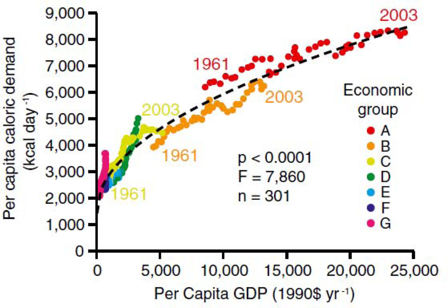

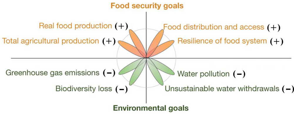
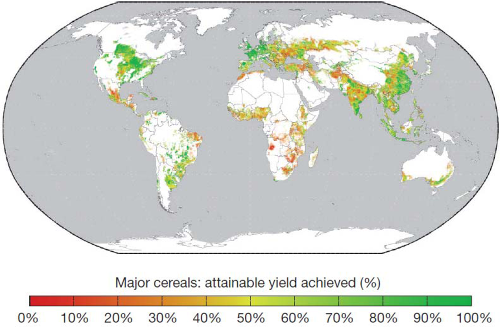
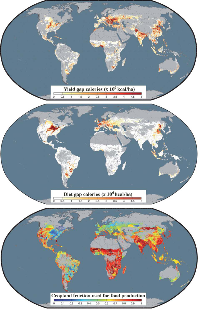
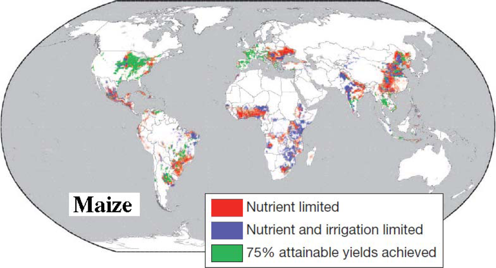

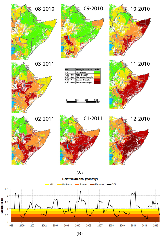
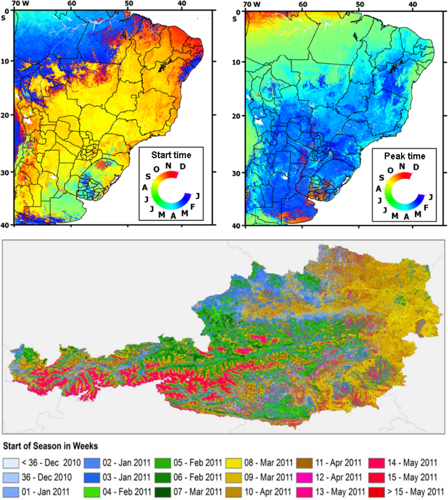
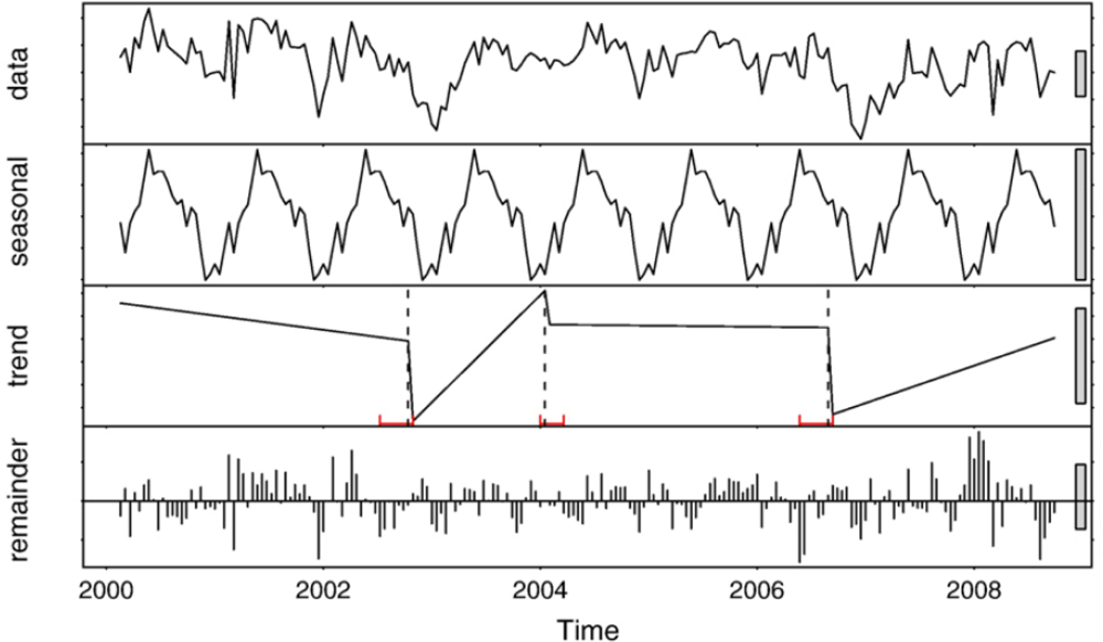
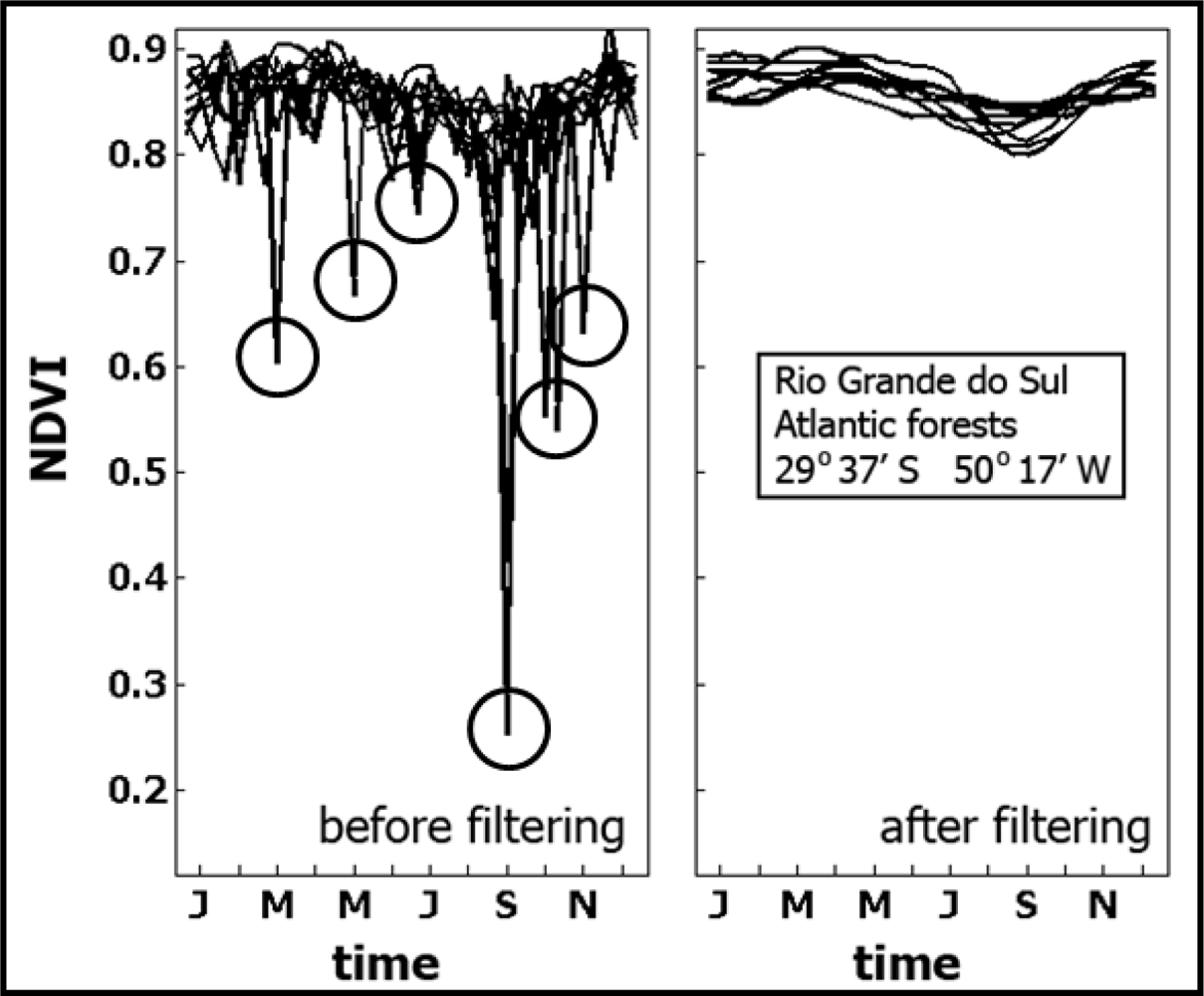
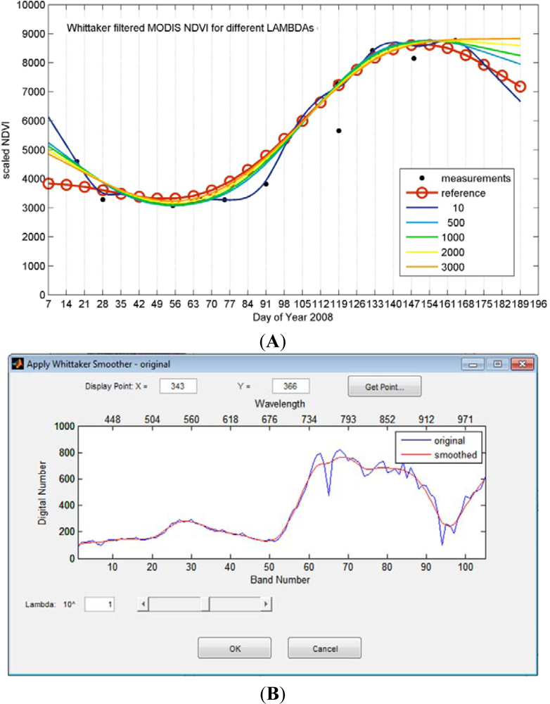
Share and Cite
Atzberger, C. Advances in Remote Sensing of Agriculture: Context Description, Existing Operational Monitoring Systems and Major Information Needs. Remote Sens. 2013, 5, 949-981. https://doi.org/10.3390/rs5020949
Atzberger C. Advances in Remote Sensing of Agriculture: Context Description, Existing Operational Monitoring Systems and Major Information Needs. Remote Sensing. 2013; 5(2):949-981. https://doi.org/10.3390/rs5020949
Chicago/Turabian StyleAtzberger, Clement. 2013. "Advances in Remote Sensing of Agriculture: Context Description, Existing Operational Monitoring Systems and Major Information Needs" Remote Sensing 5, no. 2: 949-981. https://doi.org/10.3390/rs5020949