Mapping Tropical Rainforest Canopy Disturbances in 3D by COSMO-SkyMed Spotlight InSAR-Stereo Data to Detect Areas of Forest Degradation


Abstract
: Assessment of forest degradation has been emphasized as an important issue for emission calculations, but remote sensing based detecting of forest degradation is still in an early phase of development. The use of optical imagery for degradation assessment in the tropics is limited due to frequent cloud cover. Recent studies based on radar data often focus on classification approaches of 2D backscatter. In this study, we describe a method to detect areas affected by forest degradation from digital surface models derived from COSMO-SkyMed X-band Spotlight InSAR-Stereo Data. Two test sites with recent logging activities were chosen in Cameroon and in the Republic of Congo. Using the full resolution COSMO-SkyMed digital surface model and a 90-m resolution Shuttle Radar Topography Mission model or a mean filtered digital surface model we calculate difference models to detect canopy disturbances. The extracted disturbance gaps are aggregated to potential degradation areas and then evaluated with respect to reference areas extracted from RapidEye and Quickbird optical imagery. Results show overall accuracies above 75% for assessing degradation areas with the presented methods.1. Introduction
The need to conduct research on tropical forest degradation emerged in the 1990s, as the spatial extent of selective logging and fire damage was found not to be accounted for in deforestation studies. Later, in the frame of the Kyoto protocol, reducing emissions from deforestation and degradation in developing countries (REDD) was adopted as a mechanism for the post-Kyoto reporting and parties agreed to an evaluation process by initiating REDD pilot projects. The need to address and monitor degradation along with deforestation has been emphasized on numerous occasions, such as at the COP meeting in Bali, 2007 (FCCC/CP/2007/6), where the parties “acknowledge that forest degradation also leads to emissions, and needs to be addressed when reducing emissions from deforestation”. In the Congo basin, degradation is considered more important than for example in Latin America or Asia, thus the ‘COMIFAC position on the international issue on REDD’ calls for “factoring of degradation as much as deforestation in emission calculations”.
Many definitions of forest degradation exist in the literature; a selection of definitions is provided on the FAO website [1]. Since no common definition has been yet agreed upon within the REDD+ monitoring system [2], in this study a forest degradation area is defined as an area affected by forest canopy disturbance in terms of gaps, logging roads and skid trails, where no distinction is made between man-made and natural gaps.
The use of remote sensing data to detect forest degradation is still in an early phase of development. The main obstacles when mapping tropical forest disturbances are the complex nature of forest degradation patterns and the frequent cloud cover in tropical areas. Up to now, most studies on tropical forest degradation have been based on optical imagery. Early studies in the Amazon basin investigated the degradation mapping potential of Landsat imagery by applying visual interpretation [3,4]. Extensive studies in Central Africa used Landsat imagery from three decades to derive area estimates of land cover change. A systematic regional sampling scheme based on high spatial resolution imagery was combined with object-based unsupervised classification techniques [5] to track the progression of logging roads and to track skid trails and tree felling [6]. Other methods comprise band-by-band and textural analysis [7]. Promising results were achieved by deriving cover-type fraction images using Spectral Mixture Analysis (SMA) [8]. In subsequent studies, the SMA fraction images were combined with contextual analysis, which takes into account that logging is spatially bound to either logging decks [9] or skid trails [10]. An overview of different remote sensing methods tested and validated for degradation mapping is provided in [2]. A recent review of remote sensing data sources for REDD+ monitoring is provided in [11].
The poor availability of suitable optical EO data due to frequent cloud cover in the tropics can be overcome by testing the applicability and utility of active remote sensing sensor data for degradation mapping. Surveys using SAR data specifically for forest degradation mapping are limited. The capabilities of multi-temporal single polarization SAR (e.g., ERS, JERS) backscatter texture for forest/non-forest differentiation in supervised classification methods or in unsupervised clustering have been shown in the literature [12,13]. Classification accuracies of over 90% for the classes ‘primary forest’, ‘secondary forest’, ‘recently deforested areas’ and ‘pastures’ were reported in [14] using NASA’s airborne radar system AirSAR, which acquired C-band, L-band, and P-band polarimetric data combining two frequency bands. Direct biomass assessment from ICESat/GLAS data for tropical peatland forest was done by [15] reaching an R2 of 0.61 compared to in situ aboveground biomass (AGB) measurements.
It has been demonstrated in previous studies that X-band radar data from COSMO-SkyMed [16] and TerraSAR-X [17] missions can provide useful information on forest cover and forest parameters. These sensors are able to collect images with a ground sampling distance (GSD) down to 0.75 m in Spotlight mode at various look angles. In addition, they deliver imagery with very precise pointing accuracy [18,19] so that remote regions where no reference data, i.e., ground control points, is available can also be mapped and processed, which is particularly important for vast tropical forest areas. The presented approach to digital surface model extraction for forest assessment is based on the authors’ previous works [20,21] where 3D surface reconstruction was performed by stereo-radargrammetry in Europe. Since the early years of SAR remote sensing stereo-radargrammetric techniques have been applied to SAR image pairs [22]. Currently, the methodology is again frequently used due to new SAR sensors, such as Radarsat-2 [23], COSMO-SkyMed [24] or TerraSAR-X [25]. In [26] the multi-image matching concept for digital surface modeling has been transferred from the authors’ previous work based on optical satellite images [27] to radar data, incorporating the SAR specific image geometry for forest parameters in European test sites.
2. Data and Test Site
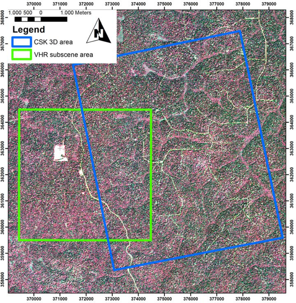
Our approach to 3D mapping of forest degradation was tested in two tropical forest areas of Central Africa within the projects REDDAf (Reducing Emissions from Deforestation and Degradation in Africa, EC FP7) [28] and GSE FM REDD (GMES Service Elements for Forest Monitoring-Extensions for REDD, ESA) [29]. Both sites were predefined as test sites for various research activities within the projects and were not specifically selected for the needs of our presented study. Reference data availability is a common problem in the tropics and due to the frequent cloud cover, VHR reference data shortly after the logging event was only available for a small area of one of our test sites. However, both sites are covered by HR RapidEye data and both show recent degradation patterns. The location of the two test sites is shown in Figure 1.
The first test site comprises the hilly terrain of the Pallisco concession area in the Eastern Province of Cameroon, where selective logging is performed. The area of the test site is 5,250 ha. A visual inspection of RapidEye data from 2008 to 2011 showed that logging activities were carried out between December 2009 and December 2011. Degradation caused by selective logging is visible in RapidEye data acquired on 5 December 2011 (see Figure 2). Based on this information, two InSAR pairs from COSMO-SkyMed (CSK) spotlight data were ordered for stereo analysis and acquired on 5 and 6 December 2011, and on 11 and 12 January 2012. Due to an intersection angle of 12.0° between the two InSAR pairs a 3D mapping procedure was applied as described in Section 3. In addition to the RapidEye scene from December 2011, a Quickbird VHR sub-scene from 2 December 2010 covering only part of the CSK area was ordered as further reference (see Figure 2).
The second test site has a size of 8,550 ha, is located in the Republic of Congo (RoC), and shows large scale degradation patterns in an area of flat terrain. Logging activities took place from early 2009 to December 2010, which can be seen from Landsat and RapidEye imagery. Again, two CSK InSAR spotlight pairs were ordered. CSK acquisitions are from 24 and 25 January 2011 and 29 and 30 January 2011. The stereo intersection angle of the InSAR pairs is 11.6°. RapidEye imagery was available from December 2009 to March 2011 and three scenes from December 2009, January 2010 and December 2010 were used as visual reference for mapping logging activities. VHR data was not available for the time after logging activities took place.
Another study site not showing any recent logging activities was to be included in our study to test the method’s suitability in non-degraded forest. Unfortunately, only one image (no stereo data) could be acquired for this site by COSMO-SkyMed. Such an analysis should be included in future studies. A summary of the data sets used in this study is given in Table 1.
3. Methods
Starting from SAR images, DEMs can be generated by exploiting either the amplitude (radargrammetry) or the phase of the radar signal (interferometric techniques). To generate digital surface models (DSMs) from radar imagery we employed an algorithm that combines interferometric processing with radargrammetry. The main idea, sketched in [31], is based on acquiring two interferometric image pairs (i.e., four complex images) at two distinct incidence angles over the scene of interest. The two InSAR pairs are processed individually and the amplitude images of the two resulting (flat terrain filtered) interferograms then serve as the two input images for stereogrammetric processing. The main advantage of using the interferogram amplitude for stereo processing is that speckle-noise can be reduced leading to higher matching accuracies. Moreover, the standard interferometric DEM generation can be applied to the coherent parts of each interferogram. Finally, the interferometric DEMs and the stereometric DEM can be merged as they show complementary behavior:
the stereometric DEM is more accurate and complete for dense vegetated areas where the interferometric coherence and thus the interferometric phase signal is low;
the stereometric DEM is less accurate and complete for open areas where the interferometric coherence and thus the interferometric phase signal is high.
Unfortunately, the used COSMO-SkyMed scenes show nearly no coherence (below 1.25% of the scene shows coherence values above 0.3) and therefore interferometric DEMs could not be generated or merged in the current study. Interferometric coherence can be of great value in forest segmentation and deforestation detection since regions of vegetation suffer from temporal decorrelation (see also the detailed study on interferometric decorrelation [32]). However, due to the low coherence values of the COSMO-SkyMed scenes, the coherence images could not be used as meaningful additional information to detect forest disturbances in our study.
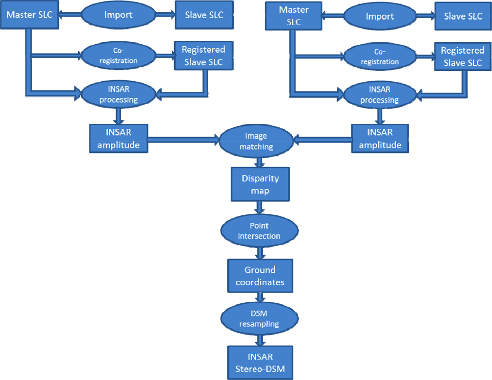
The processing chain for combined InSAR Stereo DSM extraction is illustrated in Figure 3. Co-registration is done by complex cross-correlation, a subsequent surface fitting and finally an iterative least squares adjustment. Interferograms are generated by cross-correlating the co-registered images. The results are an initial interferogram, the interferogram’s amplitude and a coherence image. The interferogram’s amplitude is then used as the input for the stereo processing. The two amplitude images are matched in order to find point correspondences. The proposed approach is based on image pyramids, where the results, i.e., the disparities, are calculated on the smaller image pyramid level and are then projected to the next larger pyramid level for refinement [33]. The next step is the spatial point intersection, i.e., an iterative least squares approach to find the 3D intersection point of SAR range circles as defined by the corresponding image pixels delivered from image matching. This methodology has also been applied successfully to optical imagery [27]. Finally, DSM resampling or rather re-gridding, i.e., interpolation of a regular raster of height values from these 3D points is performed. Remaining gaps are filled using linear interpolation of the neighboring height values. The presented approach yields a dense digital surface model, describing the surface of the region of interest.
The resulting DSMs have a spatial output resolution of 2 m. The accuracy of the DSMs could not be verified for our test sites for lack of ground truth or LiDAR DSM data, but previous studies by the authors on European forest test sites have shown geo-location errors of ±5 m and underestimations of canopy height of 2 m with respect to LiDAR using comparable stereo data [26].
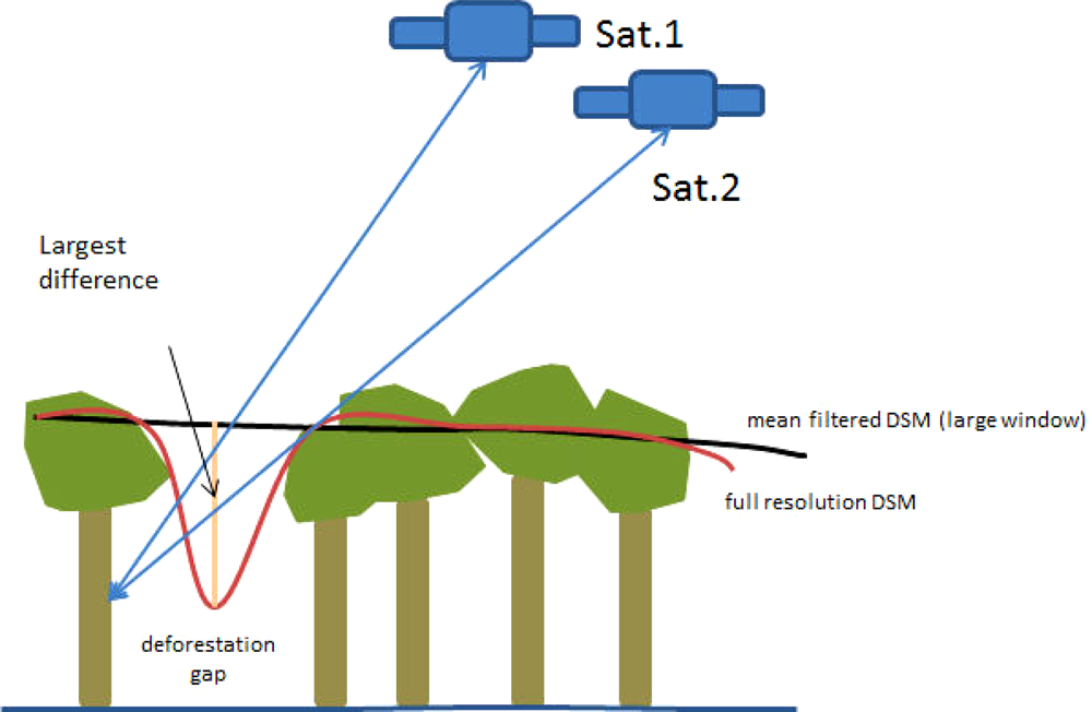
After DSM generation we tested two different approaches to derive forest disturbance from the 3D models. The first approach termed Height Variance Approach aims at detecting disturbances within the forest canopy and is based on a difference model between the full resolution surface model and a flattened mean filtered (window size >100 pixels) surface model. The method is sketched in Figure 4. Pixels with high difference values are then extracted with visually derived threshold values, e.g., all degradation features in the reference images have values of >10 m in the difference image, and serve as a preliminary forest disturbance mask. This mask is then aggregated using site specific distance and area values to map potential degradation areas.
While the Height Variance Approach shows good results for mapping larger forest disturbances related to forest roads and logging activities in the topographically flat RoC test site, it was not useful for the hilly degradation site in Pallisco. When topographic height variance within the filter window is equally large or larger than the tree height this method will fail. In addition, with this approach non-forest areas (e.g., wetlands) are falsely detected as potential degradation areas and need to be eliminated by other methods such as a supervised classification making the approach more complex and time-consuming.
We therefore used a different approach termed SRTM Difference Approach for the Pallisco test site which includes the 90 m SRTM model as the coarse surface model input instead of mean filtering the original CSK 3D model. The SRTM model reflects the topography such that height variances in the difference model are likely to represent forest disturbances and not topographic effects. This assumption was tested for our test site in Pallisco by comparing the results with logging activities visible in the RapidEye and Quickbird reference images.
The extracted individual forest disturbance polygons are then aggregated to larger polygons of potential degradation areas using the ‘Aggregate Polygons’ tool of ESRI ArcGIS software based on site specific distance values related to logging activities. The aggregation procedure combines polygons (disturbance areas) within a specified distance to create new polygons (degradation areas). By measuring distances in the Quickbird reference, an aggregation distance of 180 m was found to be a maximum distance between individual logging sites where selective logging is carried out. This means neighboring individual forest disturbance polygons with distances below 180 m are united to create a larger potential forest degradation polygon, which includes the area in between. An equal distance is applied to visually extract the reference degradation area from RapidEye data. The minimum area for the aggregated degradation area was set to 10 ha and the minimum size of a polygon hole to be retained to 50 ha.
Reference data for degradation was derived by visually identifying forest disturbances in HR RapidEye imagery and for Pallisco partly from VHR imagery. Forest disturbances were clearly visible in the HR imagery but it was not possible to differentiate individual skid trails and logging sites at this resolution. Instead of extracting individual logging sites and gaps, we created polygons for the area affected by logging activities in accordance with REDD+ monitoring requirements [34] allowing for a site specific buffer distance of 180 m, which is a maximum distance in between logging features in the area. At the Pallisco site 63% of the area was affected by degradation and 86% for the RoC test site.
4. Results and Discussion
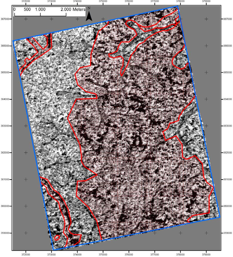
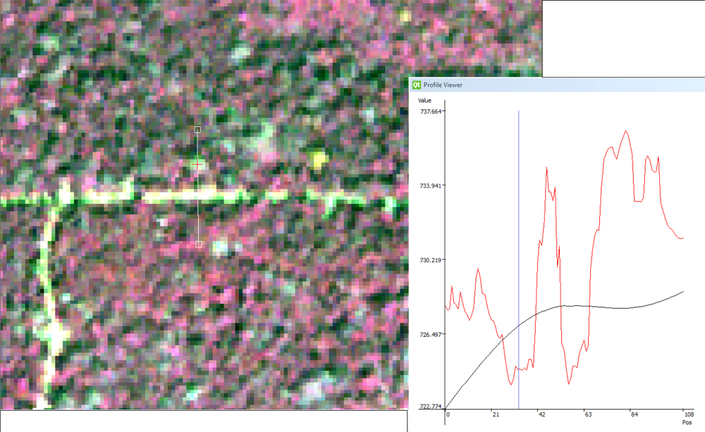
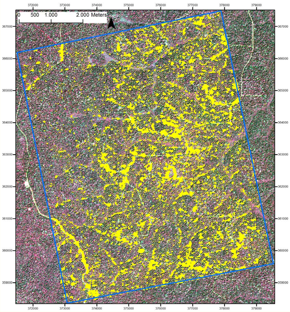
For Cameroon, only the SRTM Difference Approach was applied in the hilly Pallisco area, as the Height Variance Approach only works in flat terrain. The resulting difference model is shown in Figure 5. In areas affected by selective logging, visual reference to forest degradation from RapidEye and VHR data (area marked red in Figure 5) show that there are many patches with negative values (appearing dark in Figure 5). The basic assumption is that these values result from roads and forest gaps associated with logging. In order to test the assumption, 3D profiles of both the CSK and the SRTM model were derived over roads and forest canopy gaps, which were selected from RapidEye imagery. Figure 6 shows a profile crossing a logging road and a forest gap. Both the road and the gap show clear height differences in the two elevation models. Given these findings, an area wide estimation was performed.
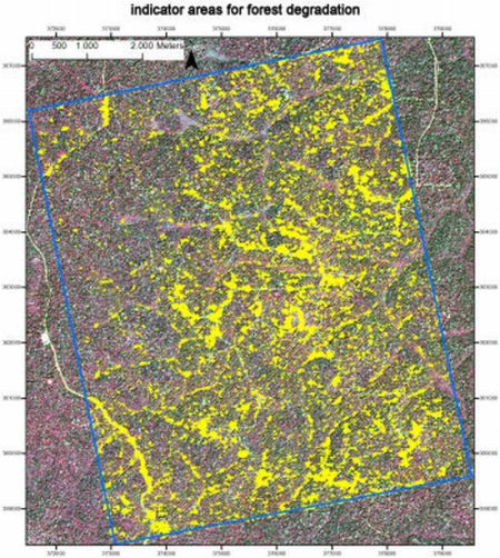
The difference model is classified into ‘areas of high difference values’ larger than 10 m (yellow patches in Figure 7); and ‘other areas’. These areas of high difference values are mostly logging roads and forest canopy disturbances and thus can serve as indicators for forest degradation. Using these indicator areas, a spatial aggregation as described above was performed to map potential areas of degradation. The output map is shown in Figure 7.
For the test site in the Republic of Congo, both the Height Variance Approach and the SRTM Difference Approach were applied. In the results of the Height Variance Approach, smaller marshlands and other non-forest areas show high difference values and are falsely included in the resulting degradation map. However, these areas are not included in the results of the SRTM Difference Approach. We have therefore combined the two resulting difference images to derive a degradation map keeping only pixels identified in both difference images as a forest disturbance and using threshold values of 8 m (Height Variance Approach) and 10 m (SRTM Difference Approach), respectively. The threshold values were derived using mean height difference values of logging roads in both models and by visually ensuring that logging roads were included in the degradation map. The difference in value between the two models seems related to the different penetration depth of the radar signal and the differing image geometries. The same aggregation procedure was applied as in the Pallisco test area.
We then evaluated our results from both test sites by comparing the aggregated degradation maps with reference degradation maps visually derived from RapidEye and Quickbird reference data. Due to the limited spatial resolution of the RapidEye data as reference, we could not derive individual gaps as reference, but instead whole forest areas affected by degradation as required by REDD+ monitoring [34]. For evaluation first a fishnet with equal grid spacing was used for all test sites, with 900 label points for the Pallisco test site and 1470 label points for the larger RoC test site. For each label point the class labels (i.e., ‘degraded forest’, ‘undegraded forest’) from the aggregated degradation maps and the reference maps were compared in a confusion matrix. The results for the different test sites and approaches are shown in Tables 2–5.
The overall accuracies vary between 75.6% and 82.0%. Overall, the degraded forest areas are underestimated. The unequal class distribution (63% and 86% degraded forest in the test sites) results in very high commission errors for the undegraded forest class and overall good accuracies for the degraded forest class. It is possible however to compare the different models for RoC. Lowest overall accuracy was achieved with the Height Difference Approach in RoC. Wetlands that occur in this test area are falsely classified as forest disturbance in the difference model resulting in the highest commission errors. By combining the Height Difference Approach with the SRTM Difference Approach in the Combined Approach, the commission error is reduced as the wetlands are eliminated from the classification of degraded forest. More than 78% of the degraded forest area was classified correctly in all images and with all approaches. The omission error for degraded forest areas of between 16.4% and 21.1% for RoC and 16.0% for Pallisco is acceptably low. The main problem is the underestimation of degraded forest and the relatively high omission and commission errors for undegraded forest, which result partly from the unequal distribution of the classes but could also result from inadequate settings for the aggregation procedure. By using a logging buffer as aggregation distance (in our study 180 m) one does not necessarily reproduce the actual shape of the logged area and the buffer can actually vary across the landscape as is pointed out in [2]. This can lead to errors in the aggregated classification with respect to the reference data. In addition, the side-looking geometry of the Cosmo-SkyMed SAR sensor leads to location inaccuracies of up to 5 m for forests [26] which can result in positional errors when combining with the SRTM model. An approach that combines ascending and descending data might reduce these geometric shifts.
All methods will need to be tested for larger areas and areas with different types of logging. Site selection for future test sites must focus on the availability of VHR data or ground truth data in order to reduce errors induced from low quality reference data. With VHR reference the produced forest disturbance maps could be compared to individual forest gaps, potentially allowing for more detailed information on logging activities, such as the length of logging road and skid trails, gap sizes and gap number. This could not be verified with the available RapidEye data.
5. Conclusion
In this study, we have tested 3D mapping approaches using COSMO-SkyMed InSAR stereo data and demonstrated their potential to map forest disturbances such as roads and gaps from selective logging in tropical forests. These disturbances, which can be considered degradation indicators, appear as large negative values in the difference images of COSMO-SkyMed digital surface model and 90 m Shuttle Radar Topography Mission model or mean filtered digital surface model. Two different methods were developed and tested at two test sites in Central Africa. The SRTM Difference Approach was tested at both sites. The Height Variance Approach requires flat terrain and could therefore only be tested at one site. Both approaches yield good results in detecting forest degradation areas with overall classification accuracies of above 75%. The accuracy for degraded forest is 78.9% for the Height Variance Approach and varies between 81.6% and 84.0% for the SRTM Difference Approach. A combination of both methods at one test site improved the overall accuracy by 2.1% compared to the SRTM Difference Approach. Due to an unequal class distribution in the reference data, the omission and commission errors for undegraded forest are very high. Future work requires the processing of an area of pristine rainforest and areas with different percentages of degraded areas in order to test whether the unequal class distribution is the main reason for the high omission and commission errors. Other sources of error could be the side-looking sensor geometry of the COSMO-SkyMed SAR sensor, which limits the matching and geo-location accuracy, and leads to a slight shift between COSMO-SkyMed and Shuttle Radar Topography Mission data. An approach that combines ascending and descending data might reduce these geometric shifts. In terms of REDD+ monitoring, however, the accuracies of the proposed procedure are well in the frame of currently achievable degradation mapping results and our proposed method has the main advantage of being independent from weather conditions for data acquisition. Further research is needed to test the performance of the proposed methods on larger areas and for different logging types.
Acknowledgments
The research leading to these results has received funding from European Union’s Seventh Framework Programme under grant agreement n°262775 (REDDAf project). Furthermore, part of these work has received funding from European Space Agency under the project GMES Service Elements for Forest Monitoring—Extensions for REDD. The COSMO-SkyMed data used was made available by the Italian Space Agency. The authors would like to thank the reviewers for their comments and suggestions, which significantly contributed to improving the quality of this paper.
References
- FAO. Forest Degradation Definitions, Available online: http://www.fao.org/docrep/009/j9345e/j9345e08.htm (accessed on 14 December 2012).
- GOFC-GOLD. A Sourcebook of Methods and Procedures for Monitoring and Reporting Anthropogenic Greenhouse Gas Emissions and Removals Caused by Deforestation, Gains and Losses of Carbon Stocks in Forests Remaining Forests, and Forestation; GOFC-GOLD: Edmonton, AB, Canada, 2009. [Google Scholar]
- Stone, T.A.; Lefebvre, P. Using multi-temporal satellite data to evaluate selective logging in Para, Brazil. Int. J. Remote Sens 1998, 19, 2517–2526. [Google Scholar]
- Nepstad, D.C.; Verissimo, A.; Alencar, A.; Nobre, C.; Lima, E.; Lefebvre, P.; Schlesinger, P.; Potter, C.; Moutinho, P.; Mendoza, E. Large-scale impoverishment of Amazonian forests by logging and fire. Nature 1999, 398, 505–508. [Google Scholar]
- Duveiller, G.; Defourny, P.; Desclée, B.; Mayaux, P. Deforestation in Central Africa: Estimates at regional, national and landscape levels by advanced processing of systematically-distributed Landsat extracts. Remote Sens. Environ 2008, 112, 1969–1981. [Google Scholar]
- Laporte, N.T.; Stabach, J.A.; Grosch, R.; Lin, T.S.; Goetz, S.J. Expansion of industrial logging in Central Africa. Science 2007, 316, 1451. [Google Scholar]
- Asner, G.P.; Keller, M.; Pereira, R.; Zweede, J.C. Remote sensing of selective logging in Amazonia assessing limitations based on detailed field observations, Landsat ETM+, and textural analysis. Remote Sens. Environ 2002, 80, 483–496. [Google Scholar]
- Souza, C.; Barreto, P. An alternative approach for detecting and monitoring selectively logged forests in the Amazon. Int. J. Remote Sens 2000, 21, 173–179. [Google Scholar]
- Souza, C.M.; Roberts, D.A.; Cochrane, M.A. Combining spectral and spatial information to map canopy damage from selective logging and forest fires. Remote Sens. Environ 2005, 98, 329–343. [Google Scholar]
- Asner, G.P.; Knapp, D.; Broadbent, E.; Oliveira, P.J.C.; Keller, M.; Silva, J.N. Selective logging in the Brazilian Amazon. Science 2005, 310, 480–482. [Google Scholar]
- de Sy, V.; Herold, M.; Achard, F.; Asner, G.P.; Held, A.; Kellndorfer, J.; Verbesselt, J. Synergies of multiple remote sensing data sources for REDD+ monitoring. Curr. Opin. Env. Sust 2012, 4, 696–706. [Google Scholar]
- Quegan, S.; Toan, T.L.; Yu, J.; Ribbes, F.; Floury, N. Multitemporal ERS analysis applied to forest mapping. IEEE Trans. Geosci. Remote Sens 2000, 38, 741–753. [Google Scholar]
- Häme, T.; Rauste, Y.; Väätäinen, S.; Ahola, H.; Stach, N.; Salvado, A. Monitoring Forest Cover in French Guiana Using Space-Borne Radar Data. Proceedings of ForestSat 2007, Montpellier, France, 5–7 November 2007.
- Hoekman, D.H.; Quinones, M.J. Land cover type and biomass classification using AirSAR Data for evaluation of monitoring scenarios in the Colombian Amazon. IEEE Trans. Geosci. Remote Sens 2000, 38, 685–696. [Google Scholar]
- Ballhorn, U.; Jubanski, J.; Siegert, F. Icesat/Glas data as a measurement tool for peatland topography and peat swamp forest biomass in Kalimantan, Indonesia. Remote Sens 2011, 3, 1957–1982. [Google Scholar]
- Agenzia Spaziale Italiana. COSMO-SkyMed System Description & User Guide; Doc. ASI-CSM-ENG-RS-093-A; ASI/Agenzia Spaziale Italiana: Rome, Italy, 2007; p. 46. [Google Scholar]
- Eineder, M.; Fritz, T.; Mittermayer, J.; Roth, A.; Boerner, E.; Breit, H. TerraSAR Ground Segment—Basic Product Specification Document; Doc. TX-GS-DD-3302; Cluster Applied Remote Sensing (DLR): Munich, Germany, 2008; p. 103. [Google Scholar]
- Bresnahan, P.C. Absolute Geolocation Accuracy Evaluation of TerraSAR-X-1 Spotlight and Stripmap Imagery—Study Results. Proceedings of Civil Commercial Imagery Evaluation Workshop, Fairfax, VA, USA, 31 March–2 April 2009.
- Raggam, H.; Perko, R.; Gutjahr, K.; Kiefl, N.; Koppe, W.; Hennig, S. Accuracy Assessment of 3D Point Retrieval from TerraSAR-X Data Sets. Proceedings of 8th European Conference on Synthetic Aperture Radar, Aachen, Germany, 7–10 June 2010; pp. 572–575.
- Raggam, H.; Gutjahr, K.; Perko, R.; Schardt, M. Assessment of the stereo-radargrammetric mapping potential of TerraSAR-X multibeam spotlight data. IEEE Trans. Geosci. Remote Sens 2010, 48, 971–977. [Google Scholar]
- Perko, R.; Raggam, H.; Gutjahr, K.; Schardt, M. Deriving Forest Canopy Height Models Using Multi-Beam TerraSAR-X Imagery. Proceedings of 8th European Conference on Synthetic Aperture Radar, Aachen, Germany, 7–10 June 2010; pp. 568–571.
- Toutin, T.; Gray, L. State-of-the-art of elevation extraction from satellite SAR data. ISPRS J. Photogramm 2000, 55, 13–33. [Google Scholar]
- Toutin, T. Impact of Radarsat-2 SAR ultrafine-mode parameters on stereo-radargrammetric DEMs. IEEE Trans. Geosci. Remote Sens 2010, 48, 3816–3823. [Google Scholar]
- Capaldo, P.; Crespi, M.; Fratarcangeli, F.; Nascetti, A.; Pieralice, F. High-resolution SAR radargrammetry: A first application with COSMO-SkyMed spotlight imagery. IEEE Geosci. Remote Sens. Lett 2011, 8, 1100–1104. [Google Scholar]
- Oliveira, C.G.; Paradella, W.R.; Silva, A.Q. Assessment of radargrammetric DSMs from TerraSAR-X Stripmap images in a mountainous relief area of the Amazon region. ISPRS J. Photogramm 2011, 66, 67–72. [Google Scholar]
- Perko, R.; Raggam, H.; Deutscher, J.; Gutjahr, K.; Schardt, M. Forest assessment using high resolution SAR data in x-band. Remote Sens 2011, 3, 792–815. [Google Scholar]
- Raggam, H. Surface mapping using image triplets—Case studies and benefit assessment in comparison to stereo image processing. Photogramm. Eng. Remote Sensing 2006, 72, 551–563. [Google Scholar]
- REDDAF. Reducing Emissions from Deforestation and Degradation in Africa: Improved Forest Monitoring Services in Developing Countries, EC FP7, Available online: http://www.reddaf.info/ (accessed on 14 December 2012).
- GSE FM REDD. GMES Service Elements for Forest Monitoring—Extensions for REDD, ESA, Available online: http://www.redd-services.info/content/gse-fm-redd (accessed on 14 December 2012).
- Verhegghen, A.; Mayaux, P.; de Wasseige, C.; Defourny, P. Mapping Congo Basin vegetation types from 300 m and 1 km multi-sensor time series for carbon stocks and forest areas estimation. Biogeosciences 2012, 9, 5061–5079. [Google Scholar]
- Raggam, H.; Gutjahr, K.; Perko, R.; Schardt, M. Assessment of the Potential of TerraSAR-X with respect to Mapping Applications Using Radargrammetric and Interferometrich Techniques. Proceedings of 3rd TerraSAR-X Science Team Meeting, Oberpfaffenhofen, Germany, 25–26 November 2012.
- Zebker, H.A.; Villasenor, J. Decorrelation in interferometric radar echoes. IEEE Trans. Geosci. Remote Sens 1992, 30, 950–959. [Google Scholar]
- Paar, G.; Pölzleitner, W. Robust Disparity Estimation in Terrain Modeling for Spacecraft Navigation. Proceedings of 11th IAPR International Conference on Pattern Recognition, The Hague, The Netherlands, 30 August–3 September 1992.
- Bucki, M.; Cuypers, D.; Mayaux, P.; Achard, F.; Estreguil, C.; Grassi, G. Assessing REDD+ performance of countries with low monitoring capacities: the matrix approach. Environ. Res. Lett 2012, 7, 014031. [Google Scholar]


| Test Site | Sensor | Attributes | Acquisition Date | Image Size | Used for |
|---|---|---|---|---|---|
| Pallisco | CSK | Spotlight, asc | 05.12.2011 | 10 km × 10 km | 3D mapping |
| Pallisco | CSK | Spotlight, asc | 06.12.2011 | 10 km × 10 km | 3D mapping |
| Pallisco | CSK | Spotlight, asc | 11.01.2012 | 10 km × 10 km | 3D mapping |
| Pallisco | CSK | Spotlight, asc | 12.01.2012 | 10 km × 10 km | 3D mapping |
| Pallisco | RapidEye | 5-band multispectral image, 5 m GSD | 30.11.2009 | 77 km × 113 km | test site selection only |
| Pallisco | RapidEye | 5-band multispectral image, 5 m GSD | 05.12.2011 | 77 km × 50 km | reference |
| Pallisco | Quickbird | (Pan&MS), Pan: 0.6 m GSD, MS: 2.4 m GSD | 02.12.2010 | 5 km × 5 km | reference |
| RoC | CSK | Spotlight, asc | 24.01.2011 | 10 km × 10 km | 3D mapping |
| RoC | CSK | Spotlight, asc | 25.01.2011 | 10 km × 10 km | 3D mapping |
| RoC | CSK | Spotlight, asc | 29.01.2011 | 10 km × 10 km | 3D mapping |
| RoC | CSK | Spotlight, asc | 30.01.2011 | 10 km × 10 km | 3D mapping |
| RoC | RapidEye | 5-band multispectral image, 5 m GSD | 01.12.2009 | 77 km × 300 km | reference |
| RoC | RapidEye | 5-band multispectral image, 5 m GSD | 20.01.2010 | 77 km × 300 km | reference |
| RoC | RapidEye | 5-band multispectral image, 5 m GSD | 10.12.2010 | 77 km × 300 km | reference |
| Reference | ||||
|---|---|---|---|---|
| classification | degraded forest | undegraded forest | user’s accuracy | |
| degraded forest | 475 | 72 | 86.8% | |
| undegraded forest | 90 | 263 | 74.5% | |
| producer’s accuracy | 84.0% | 78.5% | overall accuracy: 82.0% | |
| Reference | ||||
|---|---|---|---|---|
| classification | degraded forest | undegraded forest | user’s accuracy | |
| degraded forest | 1,033 | 78 | 93.0% | |
| undegraded forest | 233 | 126 | 35.1% | |
| producer’s accuracy | 81.6% | 61.8% | overall accuracy: 78.8% | |
| reference | ||||
|---|---|---|---|---|
| classification | degraded forest | undegraded forest | user’s accuracy | |
| degraded forest | 999 | 91 | 91.7% | |
| undegraded forest | 267 | 113 | 31.4% | |
| producer’s accuracy | 78.9% | 55.4% | overall accuracy: 75.6% | |
| Reference | ||||
|---|---|---|---|---|
| classification | degraded forest | undegraded forest | user’s accuracy | |
| degraded forest | 1,059 | 74 | 93.6% | |
| undegraded forest | 207 | 130 | 38.6% | |
| producer’s accuracy | 83.6% | 63.7% | overall accuracy: 80.9% | |
Share and Cite
Deutscher, J.; Perko, R.; Gutjahr, K.; Hirschmugl, M.; Schardt, M. Mapping Tropical Rainforest Canopy Disturbances in 3D by COSMO-SkyMed Spotlight InSAR-Stereo Data to Detect Areas of Forest Degradation. Remote Sens. 2013, 5, 648-663. https://doi.org/10.3390/rs5020648
Deutscher J, Perko R, Gutjahr K, Hirschmugl M, Schardt M. Mapping Tropical Rainforest Canopy Disturbances in 3D by COSMO-SkyMed Spotlight InSAR-Stereo Data to Detect Areas of Forest Degradation. Remote Sensing. 2013; 5(2):648-663. https://doi.org/10.3390/rs5020648
Chicago/Turabian StyleDeutscher, Janik, Roland Perko, Karlheinz Gutjahr, Manuela Hirschmugl, and Mathias Schardt. 2013. "Mapping Tropical Rainforest Canopy Disturbances in 3D by COSMO-SkyMed Spotlight InSAR-Stereo Data to Detect Areas of Forest Degradation" Remote Sensing 5, no. 2: 648-663. https://doi.org/10.3390/rs5020648
APA StyleDeutscher, J., Perko, R., Gutjahr, K., Hirschmugl, M., & Schardt, M. (2013). Mapping Tropical Rainforest Canopy Disturbances in 3D by COSMO-SkyMed Spotlight InSAR-Stereo Data to Detect Areas of Forest Degradation. Remote Sensing, 5(2), 648-663. https://doi.org/10.3390/rs5020648