Abstract
The utilization of remotely sensed observations for light use efficiency (LUE) and tower-based gross primary production (GPP) estimates was studied in a USDA cornfield. Nadir hyperspectral reflectance measurements were acquired at canopy level during a collaborative field campaign conducted in four growing seasons. The Photochemical Reflectance Index (PRI) and solar induced chlorophyll fluorescence (SIF), were derived. SIF retrievals were accomplished in the two telluric atmospheric oxygen absorption features centered at 688 nm (O2-B) and 760 nm (O2-A). The PRI and SIF were examined in conjunction with GPP and LUE determined by flux tower-based measurements. All of these fluxes, environmental variables, and the PRI and SIF exhibited diurnal as well as day-to-day dynamics across the four growing seasons. Consistent with previous studies, the PRI was shown to be related to LUE (r2 = 0.54 with a logarithm fit), but the relationship varied each year. By combining the PRI and SIF in a linear regression model, stronger performances for GPP estimation were obtained. The strongest relationship (r2 = 0.80, RMSE = 0.186 mg CO2/m2/s) was achieved when using the PRI and SIF retrievals at 688 nm. Cross-validation approaches were utilized to demonstrate the robustness and consistency of the performance. This study highlights a GPP retrieval method based entirely on hyperspectral remote sensing observations.
1. Introduction
Carbon sequestration by terrestrial ecosystems is a key factor underpinning a comprehensive understanding of the carbon budget at a global scale. Terrestrial plants fix carbon through photosynthesis, known as gross primary production (GPP) at the ecosystem scale—the largest carbon exchange between the biosphere and the atmosphere [1]. Accurate measurements and estimates of GPP will allow us to achieve improved carbon monitoring and to quantitatively assess impacts from climate changes and human activities [2,3]. Remote sensing observations provide a unique opportunity to track photosynthetic activities at various spatial and temporal scales, and much effort has been put towards this goal over the past decades. Many remote-sensing-based indices and algorithms were developed and utilized to track leaf biochemical properties (e.g., chlorophyll, water content) and canopy biophysical properties (e.g., leaf area index, LAI; absorbed photosynthetically active radiation, APAR; fraction of APAR, fAPAR) have been applied to the estimation of GPP in various ecosystems, with variable success [2,4–14]. For instance, some studies reported good performances for GPP estimation (r2 = 0.67 to 0.95) for agricultural sites [6,14] and grasslands [13] while less than satisfactory results (r2 < 0.48) have been found for hardwood forests [13].
The light use efficiency (LUE) model [15,16] has been widely utilized and coupled with remote sensing data to estimate GPP at various spatial scales [17–22], including the Moderate Resolution Imaging Spectroradiometer (MODIS) Terra/Aqua satellite GPP Products [5,23,24]. The LUE concept measures the ability of vegetation to utilize atmospheric carbon dioxide (CO2) and solar energy to produce biomass, and is usually defined as the ratio of GPP to APAR over a given period of time:
Whether based on biomass accumulation over full growing seasons as originally formulated or as instantaneous flux measurements, LUE is highly variable among different species and over phenological and environmental conditions. Instantaneous estimates of LUE are especially vulnerable to large uncertainties when used in GPP modeling [3,18,21,22,25,26]. For simplicity, the maximum expected LUE (LUEmax) has often been used to model GPP (e.g., MODIS GPP Product), but this approach requires considerable environmental information to down-scale from assumed optimal values to predict actual ones [23,24] and to describe GPP under non-optimal, unfavorable environmental conditions.
LUE has been shown to be closely correlated to biochemical responses related to photoprotection of plant tissues, when more solar radiation is absorbed than can be utilized for photosynthesis [27]. One such process is non-photochemical quenching (NPQ), regulated by the xanthophyll cycle, in which the pigment violaxanthin is reversibly de-epoxidized to zeaxanthin via antheraxanthin [18,27–33]. The xanthophyll cycle can be monitored with the Photochemical Reflectance Index (PRI), a normalized difference band ratio based on the narrow spectral bands centered at a physiologically active 531 nm response and a reference band insensitive to the xanthophyll signal (e.g., 570 nm), as proposed by Gamon and colleagues [32,34]. The capability of the PRI to track photosynthetic activities, including LUE, has been investigated across plant functional types at leaf, canopy, and landscape levels using various instruments [19,20,29,32,34–41]. Moreover, many recent studies have investigated various factors that influence the PRI:LUE relationship at canopy or ecosystem scales including viewing geometry, canopy structure, leaf area index (LAI), soil background, pigment content (e.g., carotenoids/chlorophyll ratio), and shadow fraction [17,18,21,22,42–51].
Another important photoprotection process is chlorophyll fluorescence, where excessive energy is expelled in order to prevent harmful photo-oxidation [3,18,28,32]. Decades of laboratory studies and recent field-based solar-induced fluorescence (SIF) studies have shown that fluorescence provides a direct indicator of plant photosynthetic function (e.g., carbon fixation), enabling early detection of environmentally induced stress [52–60]. However, retrieving the SIF signal from passive remote sensing spectral observations over vegetation canopies under ambient solar illumination has been challenging because it is a weak signal added to the reflected radiance. Nevertheless, recent studies have shown success for SIF retrievals at leaf, canopy, and even satellite levels. Previously, since the SIF signal is small and requires very high spectral resolution for retrieval, attempts were made to develop optical reflectance-based approaches for SIF [61–65]. In contrast to these relative indices, radiance-based algorithms enable direct estimates of SIF in physical or arbitrary units [54,55,66–70].
The chlorophyll fluorescence emission spectrum occurs across the red and near-infrared spectral region (650–800 nm) with two peaks near 685 nm and 740 nm. Radiance-based SIF retrieval approaches utilize measurements within and around atmospheric Fraunhofer lines that overlay the emission window to decouple SIF from reflected radiance. This is possible because the SIF signal contributes more to reflected radiance from vegetation canopies within these narrow dark lines where irradiance is low because of strong atmospheric absorption [54,55,57]. The two telluric oxygen bands, O2-A (centered at 760 nm, ∼7 nm width) and O2-B (688 nm, ∼4 nm width) bands, are the most exploited absorption features for SIF retrievals. Many studies have reported that SIF can be detected using this passive remote sensing based concept [26,54,69,71–75]. The successful SIF retrievals to date have utilized the far-red (O2-A) retrieval to improve estimates and/or reduce uncertainty of photosynthetic activities, LUE and GPP, at leaf [76] and canopy levels [26,60,73,74,77]. However, few studies have successfully retrieved red fluorescence from the O2-B feature, nor have they examined red fluorescence in conjunction with canopy GPP measurements.
The fluorescence emission and NPQ energy dissipation are important components in the carbon fixation machinery of plants. The two processes are considered to be photosynthetic stress indices under sub-optimal environmental conditions and direct probes of plants’ physiological and photosynthetic status [29,32,53–56,78–81]. In recent years, advances in remote sensing technology, especially those providing higher spectral resolution and signal-to-noise ratio, have enabled retrievals from high spectral resolution optical observations that correlate to the two dissipative pathways. Since both NPQ and chlorophyll fluorescence provide information relevant to photosynthetic activities (e.g., LUE and GPP) at the canopy scale [54,82,83], further investigations are warranted. In particular, the relationships among photosynthesis, PRI, and SIF derived from remote sensing observations, need further investigation, including examination of the red SIF. Several recent studies investigated the use of PRI and SIF to model LUE and GPP with various success [26,73,74,78], but the mechanism linking PRI and SIF to each other and to GPP is not yet well-described. In the current study, we introduce a collaborative field campaign conducted in a cornfield during four years. Hyperspectral observations and eddy covariance measurements were acquired during each year of the campaign. The study aims to investigate a greater range, both diurnal and seasonal changes, than previous publications. The study was undertaken to examine the capability of PRI and both far-red and red SIF to model the diurnal variations of two important photosynthetic parameters, LUE and GPP for multiple growing seasons.
2. Methods
2.1. Study Site and Field Data Collection
The study site is located within the Optimizing Production Inputs for Economic and Environmental Enhancement (OPE3) experimental field (39.030°N, 76.845°W) maintained by the USDA Beltsville Agricultural Research Center (BARC) in Maryland, USA. Field campaigns were conducted on corn (Zea mays L.); different corn cultivars were planted during each of the four growing seasons in 2008, 2010, 2011, and 2012 (Table 1). Measurements were made on a total of 30 sunny days spanning different growth stages, ranging from early vegetative stages when the corn crop was actively growing at ∼1 m tall and had produced 7–9 leaves (e.g., V7, V9) to fully mature canopies in the reproductive stage at ∼2 m tall (e.g., VT, R1), through advanced reproductive development in the senescent stage (e.g., R4, R6). On each field day, measurements were taken multiple times between 9 am to 6 pm local time with approximately one-hour intervals, to sample the diurnal course. Sampling was done every one meter along a marked 100 m north-south direction transect in the middle of the field to minimize disturbance to the field. One complete set of sampling the transect was usually done within 30 min. Average of the samples was calculated to represent the field for the specific sampling time [84].

Table 1.
Information about crop and environmental conditions in the USDA experimental cornfield in the four growing seasons. Dates are in the format of day of year (DOY). Total precipitation and average temperature are for the time period in Figure 1. Gross primary production (GPP) is in the unit of g CO2/m2/d.
Canopy level hyperspectral reflectance spectra (400–1,000 nm, ∼1.5 nm Full Width Half Maximum; FWHM) were obtained using a USB4000 Miniature Fiber Optic Spectrometer (Ocean Optics Inc., Dunedin, FL, USA) with a bare fiber. All spectral observations were acquired at nadir, above the canopy at a height of approximately 1 m. This was accomplished by placing the fiber optics on a height-adjustable pole-mount, where a custom-made fixture was designed to position the instrument at a desired view zenith angle and relative azimuth angle [85]. Incident solar irradiance was determined using a Spectralon reference panel (Labsphere, North Sutton, NH, USA). Incident solar irradiance was measured in between approximately every five samples. An additional spectrometer was set up to measure the reference panel continuously to monitor detailed changes of irradiance during the field days. Supplemental measurements included LAI and fPAR. LAI was measured with the LI-COR LAI-2000 plant canopy analyzer (LI-COR, Lincoln, NE, USA) and fPAR was determined using the LI-COR LI-191 line quantum sensor (LI-COR, Lincoln, NE, USA).
2.2. Spectral Data Processing
The PRI is usually calculated using two green bands at 531 nm and 570 nm as a normalized index [32,34]:
In this study, we used canopy reflectance acquired over corn canopies centered at 531.01 nm and 570.08 nm at their native FWHM of 1.5 nm to calculate the PRI. The O2-A (760 nm) and O2-B (688 nm) absorption features were utilized to derive SIF signals in this study. The fluorescence retrievals were determined using a modified Fraunhofer line depth (FLD) algorithm [66] on the spectral observations over corn canopies. The FLD principle [86] utilizes incident solar irradiance and radiance measurements reflected off vegetation canopies. By comparing the measurements inside and outside (reference band) an absorption feature, the estimate of fluorescence is derived. The modified FLD algorithm [66] utilizes measurements on both shoulders (instead of one, the left shoulder) of an absorption feature to construct the reference band for a more realistic description [54,70]. Detailed description and review of different algorithms to retrieve SIF can be found in previous publications [54,67,70]. In this study, we utilized the bands centered at 685.57 nm, 687.11nm, and 691.77 nm for red fluorescence retrievals and the bands at 757.86 nm, 760.86 nm, and 772.67 nm for far-red fluorescence retrievals. These bands are at the native sampling resolution of the instrument of approximately 0.2 nm. We use SIF (red) to denote retrievals derived in the O2-B feature centered at 688 nm and SIF (far-red) for retrievals within the O2-A feature centered at 760 nm. Since values for SIF retrievals are also affected by the intensity of irradiance, we also derived SIF yield, a dimensionless quantity that is independent of the light level. SIF yield was calculated following methods developed in a previous study [57] as the ratio of SIF retrievals and the measurement outside the absorption feature (reference band) from irradiance, denoted as SIF (red) yield in the O2-B band region and SIF (far-red) yield for the O2-A feature. Normalized Difference Vegetation Index (NDVI) was calculated using red (620–670 nm) and near-infrared (841–876 nm) bands similar to the spectral characteristics of MODIS land surface reflectance.
2.3. Flux Data, LUE and GPP Modeling
The cornfield is equipped with a 10 m high eddy-covariance-instrumented tower that measures fluxes from a field approximately 16 hectares in area. Our sampling was approximately 65 m away from the flux tower and within the footprint. Flux data are reported at 30 min intervals throughout all 24-h periods of the full growing season. Net Ecosystem Production (NEP) is determined from the measured net CO2 exchange using the eddy covariance method, supported by the tower’s micro-meteorology measurements (e.g., PAR, temperature, wind speed and direction, precipitation). Data were processed following the FluxNet/AmeriFlux guidelines [87], and the NEP was partitioned into respiration and GPP [88], compatible with AmeriFlux standards. Air temperature was measured at four meters above the ground on the flux tower and reported at half-hourly intervals. Precipitation was measured with a tipping rain gauge mounted one meter off the ground at a USDA/BARC meteorological station.
Corresponding flux data were extracted when spectral observations were made on each field day. A combined flux and optical dataset was used to examine the potential of modeling LUE and GPP as the product of PRI, SIF (red and far-red), or both optical variables. This goal was accomplished through linear regression analyses with the R language and software by JMP (SAS Institute Inc., Cary, NC, USA). The general model formulations are listed in Table 2.
Table 2.
General formulation of the light use efficiency (LUE) and GPP flux parameters examined in this study, developed using the Photochemical Reflectance Index (PRI) and solar induced chlorophyll fluorescence (SIF) optical variables acquired in the USDA Beltsville Agricultural Research Center (BARC) cornfield. Note: a, b, c, d, represent coefficients of the linear regression models from statistical analyses.
2.4. Cross-Validation
To evaluate the performance of the experimental models, cross-validation procedures were utilized. First we used the k-fold cross-validation approach. This method partitions the data into k subsets, then uses (k − 1) subsets as the training set to fit the model while the validation is conducted using the omitted subset. In this study, the k value was set to 10 and the dataset was randomly divided into 10 subsets of equal sample size. The process was repeated 10 times to assess the coefficient r2cv and RMSEcv for performance evaluation. Secondly, we partitioned the dataset in a more restrictive manner, utilizing the 2008 data (roughly half of the entire dataset) as the training data versus the 2010 through 2012 data as the validation data. This strategy was invoked to assess the consistency of the model in the temporal domain.
3. Results
3.1. Diurnal and Seasonal Courses of GPP, PRI, and SIF
The different cultivars planted each year produced variable leaf area indices (LAI) and maximum mid-season GPP, having been influenced by planting date and environmental conditions (Table 1). Daily GPP derived from tower-based eddy covariance measurements in the cornfield over four growing seasons is shown in Figure 1a. The grey dashed lines indicate the days when field campaigns were conducted. Corresponding daily precipitation, daily PAR, and daily average and high temperature observations are reported in Figure 1b–d, respectively. Clear seasonal dynamics were observed for GPP, which increased during the green-up vegetative stage, reached the highest productivity during mid-season, and steadily declined after that (Figure 1a). Within this general seasonal trend, an increase in GPP was usually observed after a noticeable precipitation event (Figure 1a,b). The highest mid-season GPP value (∼75 g CO2/m2/d) was observed in early August of 2008 and in mid-July of 2010 (Figure 1a; Table 1), and comparable GPP values and seasonal patterns were observed in those two years. Lower maximum mid-season GPP values were observed in 2011 and 2012, mostly due to unfavorable environmental conditions, such as unseasonably high temperature and/or lower precipitation (Figure 1b,d).
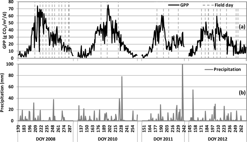
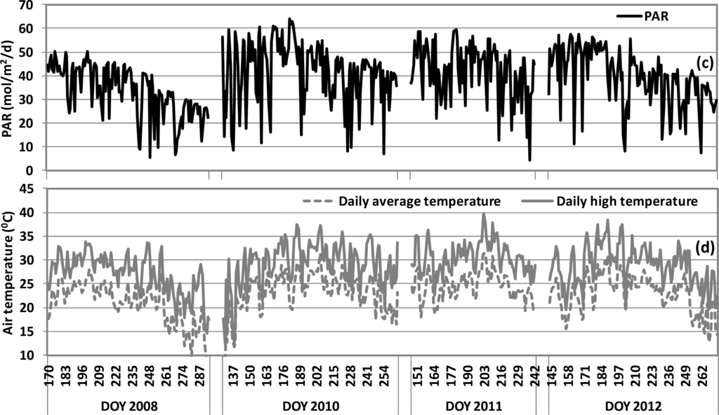
Figure 1.
Seasonal variations of (a) daily GPP (g CO2/m2/d); (b) daily precipitation (mm); (c) daily PAR (mol/m2/d); (d) daily average and high air temperature in USDA BARC OPE3 cornfield for four growing seasons. X-axis values indicate day of year (DOY) in 2008, 2010, 2011, 2012. The vertical dashed grey lines in panel (a) indicate field days.
Our dataset consists of a total of 30 days of carbon fluxes and spectral observations. The diurnal patterns of GPP, LUE, SIF (red), and PRI are shown in Figure 2a–d, respectively, for a sample dataset of eight days. In general, all four variables showed different maximum (or minimum) values and clearly expressed diurnal dynamics (Figure 2). Lower GPP values occurred in early morning and late afternoon, and higher values occurred around mid-day, in concert with illumination and air temperature changes (Figure 2a). In contrast, LUE exhibited higher values in early morning and late afternoon, with lower values during mid-day, indicating lower efficiency due to mid-day thermal or moisture stress (Figure 2b). SIF (red) and GPP exhibited similar diurnal courses (Figure 2c). Diurnal changes of PRI and LUE showed similar patterns, with higher values in early morning and the late afternoon, but lower values during mid-day (Figure 2d).
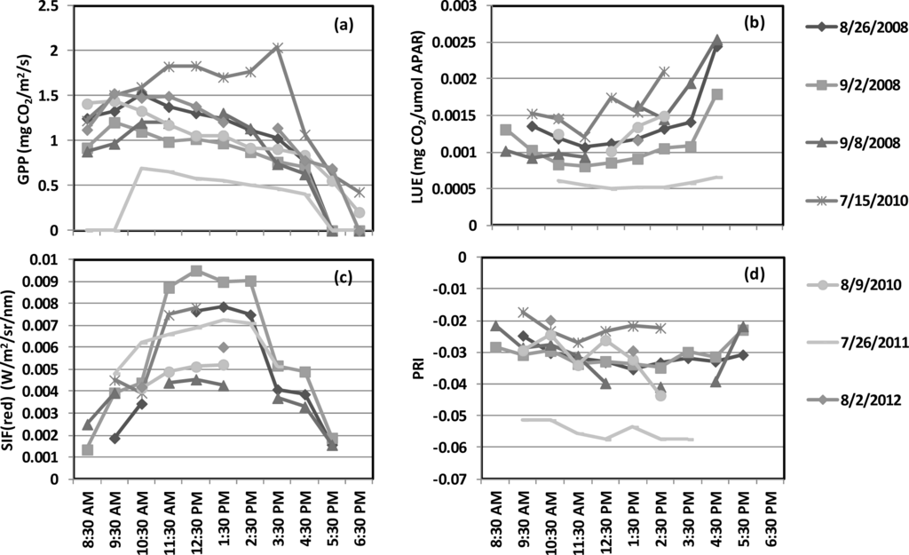
Figure 2.
Diurnal patterns of (a) GPP, (b) LUE, (c) SIF (red), and (d) PRI for selected field days in four growing season.
The seasonal changes of NDVI, PRI and SIF are shown as daily average values, along with daily GPP values, in Figure 3. NDVI expressed little seasonal change during the 2008 field season but had more variation in the other years. However, the PRI and SIF values exhibited pronounced variations in magnitude and seasonal dynamics across the four growing seasons. Towards the end of the growing season in 2008, 2011, 2012, the PRI values declined rapidly to notably lower values during the senescent stage (Figure 3). In general, the PRI and all of the SIF variables had seasonal trends similar to GPP.
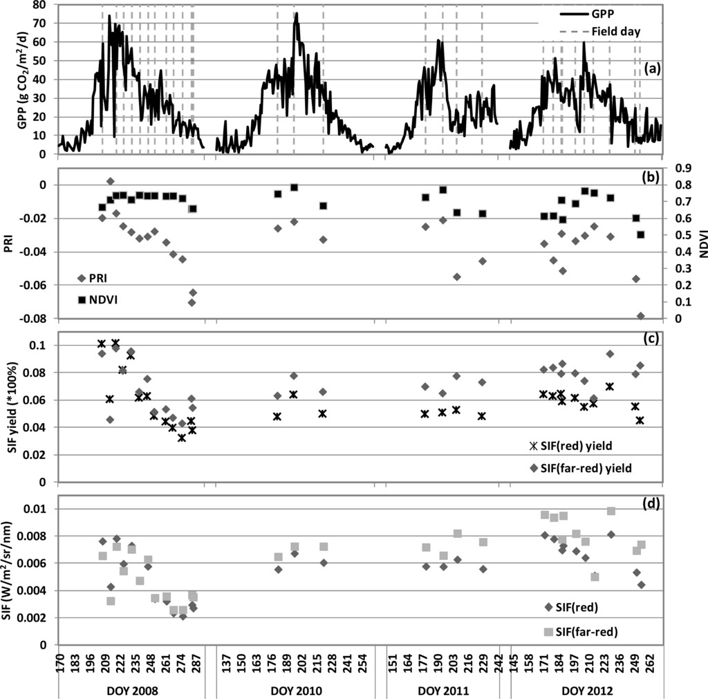
Figure 3.
Cornfield seasonal dynamics of the daily average over four growing seasons for: (a) GPP, (b) PRI and Normalized Difference Vegetation Index (NDVI), (c) SIF yield (×100%), and (d) SIF (W/m2/sr/nm).
3.2. LUE and GPP Modeling
We investigated using PRI and SIF to model two important photosynthetic parameters, LUE and GPP. The statistics of modeling LUE using PRI and SIF are summarized in Table 3. In general, SIF by itself did not generate strong relationships with LUE when examined over time. By itself, however, the PRI exhibited the best correlation with LUE (r2 = 0.45, RMSE = 0.000324 mg CO2/μmol PAR). Nevertheless, as shown in Figure 4, the relationship between PRI and LUE was not consistent among the four years (grey lines). Linear fit with r2 of 0.56, 0.69, 0.50 was found for 2008, 2011, 2012, respectively with different slopes and offsets (Figure 4). By applying a logarithm fit, a 9% improvement was observed for the PRI model over the four-years (r2 = 0.54, RMSE = 0.000322 mg CO2/μmol PAR, Figure 4, black line). By combining the PRI with any SIF variable, substantial improvements in relationships to LUE and GPP were achieved. For LUE, a 16% improvement over the linear PRI model, and a 7% further improvement over the log PRI model, was obtained for the model that combined the PRI with the SIF (red) yield (r2 = 0.61, RMSE = 0.000275 mg CO2/μmol PAR; Table 3). The statistics of modeling GPP using PRI and SIF are summarized in Table 4. For GPP, ≥24% improvements over the linear PRI model (r2 = 0.54, RMSE = 0.2770 mg CO2/m2/s) were obtained for the models that combined the PRI with either the SIF (far-red) (r2 = 0.78, RMSE = 0.1894 mg CO2/m2/s) or with the SIF (red). The SIF (red) retrieval provided the strongest performance overall (r2 = 0.80, RSME = 0.1994 mg CO2/m2/s; Figure 5; Table 4).
Table 3.
Summary of statistics (r2 and RMSE) of LUE models examined in this study. Note: the highest performing model in each group is shown in bold type.
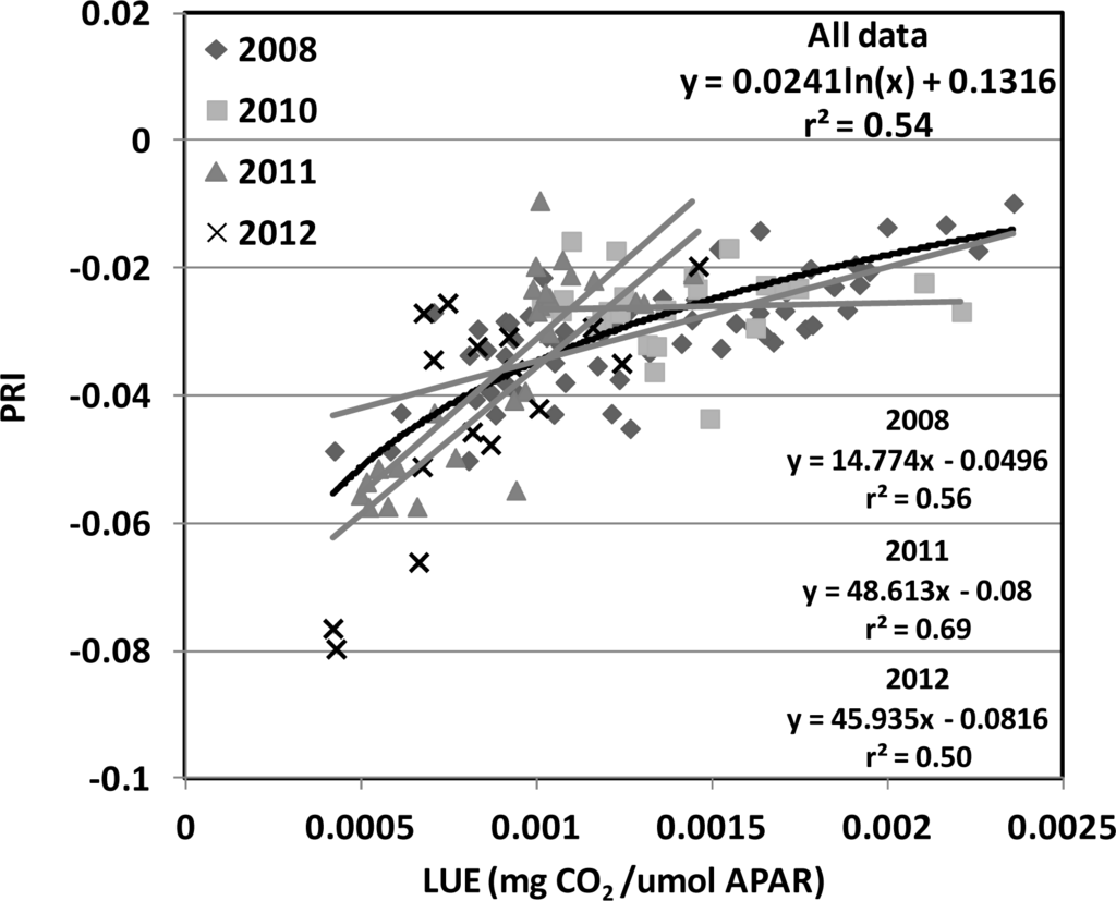
Figure 4.
Relationship between canopy PRI and flux tower-based LUE for 2008 (
 ), 2010 (
 ), 2011 (
 ), 2012(
 ) in the USDA BARC cornfield.
), 2010 (
), 2011 (
), 2012(
) in the USDA BARC cornfield.
Table 4.
Summary of statistics (r2 and RMSE) of GPP models examined in this study. Note: the highest performing model in each group is shown in bold type.
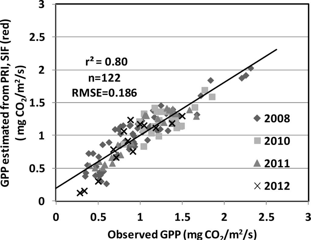
Figure 5.
Performance of the GPP model (r2 = 0.80, RMSE = 0.186 mg CO2/m2/s) using both the PRI and the SIF (red) observations from four growing seasons (2008, 2010–2012) in the USDA BARC cornfield.
3.3. Cross-Validation
The performance of the GPP models, using cross-validation procedures, was examined for the model that combined the PRI with the SIF (red), since it produced the best empirical performance. The k-fold cross-validation approach to the model (Figure 6) consistently provided satisfactory statistics (r2cv = 0.79, RMSEcv = 0.188 mg CO2/m2/s). When repeating this analysis for the same model using only 2008 data, evaluated by comparison with the remaining dataset, showed comparable results for the training data (Figure 7a) and validation data (Figure 7b). These results were also similar to the original model presented previously (Figure 5), demonstrating the consistency and robustness of the model across multiple growing seasons, including different corn cultivars and variable environmental conditions.
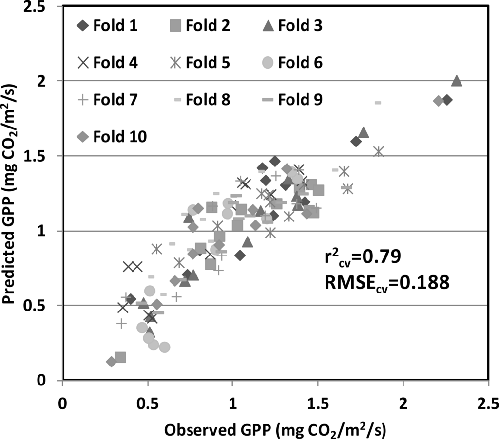
Figure 6.
Results of the k-fold cross-validation (K value set to 10) performed on the GPP model presented in Figure 5. The cross-validated r2 (r2cv = 0.79) and RMSE (RMSEcv = 0.188 mg CO2/m2/s) confirms the robustness of the GPP model using PRI and SIF (red).
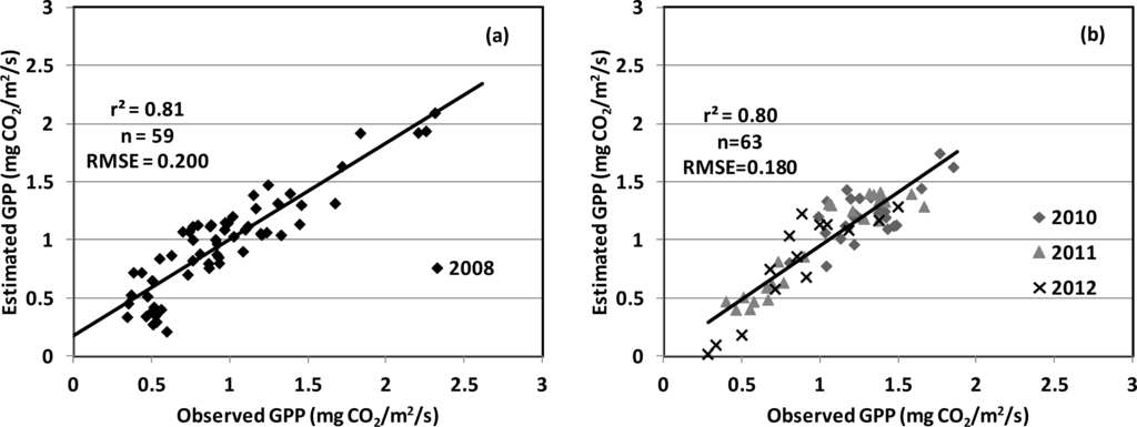
Figure 7.
Cross-validation of the GPP model presented in Figure 5 using a systematic partitioning approach: (a) data acquired in 2008 were used as training data to develop the model; and (b) data from 2010 to 2012 were used as validation data. The results confirm the consistency of the GPP model applied over four growing seasons.
4. Discussion
In this study, we examined two different types of optical remote sensing variables (PRI, SIF) to track the physiological status of plants for monitoring carbon assimilation in a cornfield. We made observations over different environmental and crop conditions in four growing seasons, which included different corn cultivars in each year.
We documented inter-annual and diurnal variations in the optical indices as well as GPP values (Figure 1), which were influenced by weather conditions. Precipitation in this rain-fed field increased GPP values. But unseasonably high temperatures, observed in the middle of the 2011 season and in 2012 during the vegetative stage, created strongly expressed canopy stress which reduced productivity and GPP. Diurnal GPP cycles showed higher mid-day production when the vegetation was exposed to abundant solar radiation. However, both the SIF and PRI responses indicated that plants experienced physiological stress during mid-day, also induced by high solar radiation and temperatures. Higher SIF and lower PRI values expressed higher stress conditions during mid-day, while lower SIF/higher PRI values described stress abatement during early morning and late afternoon (Figure 2c,d). This diurnal trend was captured in the tower-based LUE, which exhibited the opposite diurnal dynamics to GPP (Figure 2a,b). A similar pattern to diurnal trends was seen in the seasonal trends of GPP, PRI, and SIF (Figure 3). Certain growth variables (e.g., LAI, phenological stage) affected the observed values for GPP, PRI and SIF. In 2008, NDVI value remained fairly consistent across the field season. On the contrary, both PRI and SIF displayed seasonal changes in concert with GPP that year, similar to the results for a sorghum field [75]. This shows that the PRI and SIF provide information that is more related to photosynthetic function than might be inferred from the NDVI.
Several previous studies investigated similar topics and evaluated the performance of PRI and SIF for carbon monitoring. Rossini et al. [73] examined SIF (far-red) retrievals at 760 nm for fAPAR estimates, combined with either SIF yield or PRI, to model LUE in a rice field during two growing seasons; this method significantly improved estimates and reduced uncertainty in mid-day GPP (r2 = 0.91, RMSE = 3.40 μmol CO2/m2/s). Rossini et al. [74] examined various formulations that coupled a suite of spectral vegetation indices, including the PRI, to estimate mid-day and daily GPP in a subalpine grassland. Damm et al. [26] utilized SIF retrievals at 760 nm and PRI to improve LUE estimates for describing the diurnal GPP course in a cornfield. Zarco-Tejada et al. [79] reported that the PRI and SIF retrievals at the 760 nm showed a similar seasonal trend to that of GPP measured at the same time of spectral observations (r2 between 0.75 and 0.84; p < 0.01). The study reported a GPP model (r2 = 0.67, RMSE = 5.77 μmol CO2/m2/s) using LUE estimates based on the SIF (far-red) yield at 760 nm, while the PRI-based LUE exhibited weaker performance (r2 = 0.26, RMSE = 9.25 μmol CO2/m2/s) for GPP estimates. These field studies demonstrate that variable results across vegetation types and conditions can be obtained in using SIF and/or PRI to estimate LUE or GPP.
Our study addressed a similar topic: to investigate the potential use of PRI and SIF to estimate GPP, and to reduce uncertainties in the GPP and LUE estimates (Figure 5, Table 4). The models investigated and presented in our current study were composed solely of remotely-sensed observations. Unlike many previous studies, no micrometeorological variables (e.g., PAR or air temperature) were needed to achieve acceptable performance. The format of the models was determined after reviewing previous studies [26,73,74]. The models we utilized are similar to the Type 1 model in Rossini et al. [74], or the E3 model examined in Rossini et al. [73]. This confirms the potential for this type of GPP modeling approach, which has the advantage of simplifying the input data type requirements. Although most previous studies have focused on retrievals using the O2-A band to obtain SIF (far-red), we included SIF retrievals at the O2-B band feature to obtain SIF (red), which provided the strongest relationship to GPP, possibly due to its important role in photosystem II (PSII) processes [53,89]. Furthermore, we undertook the challenge to model the diurnal variation of GPP during four growing seasons, which presented a complex task since both plant physiological conditions and GPP were changing significantly within any day, as well as across the four growing seasons due to varying climate conditions (Figure 1).
The results (Tables 3 and 4) showed the challenge of modeling diurnal variations of LUE and GPP at this site for multiple growing seasons when using only PRI or SIF. Better correlations between PRI, SIF, LUE and GPP were found when using daily average values to study seasonal variations. For instance, for the 2008 growing season, when using daily average values, better performance was observed for the PRI:LUE model (r2 = 0.76), the SIF (red) yield:LUE model (r2 = 0.71), and the SIF (red):GPP model (r2 = 0.61). However, the performance changed when we made the attempt to model diurnal variations across multiple growing seasons. In general, the GPP models examined in this study performed better than the LUE models. Multiple studies have demonstrated the potential of using the PRI to track LUE and photosynthetic activities for various vegetation types (e.g., [17,18,21,22,29,50,51]). The PRI:LUE model we developed with our dataset performed adequately (r2 = 0.54) and overall results were comparable to previously published results [50]. Nevertheless, one can easily observe year-to-year variations among the four growing seasons, since many factors affect the PRI values as well as the PRI:LUE relationship, e.g., canopy structure, LAI, soil background, and pigment content [42,45,48,50,51,85]. No significant correlations were observed between SIF and either LUE or GPP for this dataset, but adding SIF to a simple PRI-based model improved its capability to track the variation in LUE by as much as 16% (Table 3). These findings suggest a future approach to significantly improve the performance of current LUE models, by combining these two optical signals.
NPQ and chlorophyll fluorescence emission are considered as direct indicators of photosynthetic activities and physiological stress when plants are under sub-optimal environmental conditions [28,53,59,80,90–93] such as low water availability [81,93–95], unfavorable temperatures [96,97], nutrients [98–101], and salinity [102,103]. Consequently, many studies have utilized the spectral indices, PRI and SIF retrievals, as indicators of stress and down-regulation of LUE and GPP [29,50,51,65,82,92,104–107]. Our results lend support to those reported from previous studies that demonstrated that PRI and SIF retrievals were correlated to two important protective mechanisms (NPQ and chlorophyll fluorescence emissions), discarding excess absorbed solar radiation that could not be used in photosynthesis [3,29,54]. These might explain the empirical GPP model we presented in this study using both PRI and SIF showed good agreement with tower-based fluxes with low uncertainties. Furthermore, we achieved significant improvement by using both PRI and SIF together for GPP estimates, rather than using either PRI or SIF alone to attain a more comprehensive description of the entire carbon fixation mechanism, and hence, to deliver more accurate GPP estimates.
Cross-validation approaches are designed to evaluate the robustness and consistency of statistical models. One crucial factor about cross-validation is the strategy to divide the entire dataset into training and validation data, using a random sampling and a systematic partitioning to test our results. We demonstrate that the GPP model based on 2008 data was able to predict GPP using PRI and SIF (red) in the three other years—2010, 2011, and 2012. This highlights the robustness of the integration of PRI and SIF (red) to capture important information about physiological status of this cornfield, thus providing accurate estimates of carbon assimilation with small uncertainties. The k-fold cross-validation approach was also applied to the model with PRI and SIF (far-red), with only a slightly lower performance (r2cv = 0.77, RMSEcv = 0.205 mg CO2/m2/s). It can be difficult to retrieve SIF (red) from space [108] since it is a narrower and weaker feature than SIF (far-red), and this capability has yet to be attained. Even though our results suggested better performance of SIF (red) to model photosynthetic processes in ground level studies, we also demonstrated the potential for using SIF (far-red) for carbon monitoring using satellite measurements at global level.
5. Conclusions
In this study, we examined the capability of the PRI and SIF to track plant photosynthetic function in order to estimate diurnal variations of GPP in a cornfield over multiple growing seasons. Our results showed that the PRI and the SIF successfully captured the diurnal and seasonal dynamics in plant physiological status, in response to environmental and phenological conditions. Similar diurnal and seasonal patterns were observed for PRI and tower-based LUE as well as SIF and GPP. Although the PRI delivered the best performance (r2 = 0.54; RMSE = 0.000322 mg CO2/μmol PAR) when using a single optical variable for modeling canopy LUE, it nevertheless, was inconsistent when applied among multiple years. The most significant result was obtained by integrating both the PRI and the SIF, especially the SIF (red), in an empirical model to monitor diurnal variations in GPP for four growing seasons (r2 = 0.80; RMSE = 0.1894 mg CO2/m2/s), which showed a minimum of 26% performance improvement than using either PRI or SIF alone. The robustness and consistency of which was demonstrated by cross-validation approaches (r2cv = 0.79; RMSEcv = 0.188 mg CO2/m2/s). These results demonstrate that the PRI and SIF, utilized together, provide a powerful tool for carbon monitoring. This concept must be pursued over various vegetation types, given the success we report here for a cornfield, but we recommend more emphasis on SIF (red) retrievals in the future.
Acknowledgments
This study was supported by a NASA ROSES project (PI, E.M. Middleton) funded through the Terrestrial Ecology Program (Diane Wickland, Program Manager). The authors gratefully acknowledge Andrew Russ and Wayne Dulaney (USDA-ARS Hydrology and Remote Sensing Lab) for assisting field campaign and data processing. The authors thank the anonymous reviewers for their very valuable suggestions and critiques.
Disclaimer
The mention of trade names of commercial products in this article is solely for the purpose of providing specific information and does not imply recommendation or endorsement by National Aeronautics and Space Administration or the US Department of Agriculture.
Conflict of Interest
The authors declare no conflict of interest.
References
- Beer, C.; Reichstein, M.; Tomelleri, E.; Ciais, P.; Jung, M.; Carvalhais, N.; Rodenbeck, C.; Arain, M.A.; Baldocchi, D.; Bonan, G.B.; et al. Terrestrial gross carbon dioxide uptake: Global distribution and covariation with climate. Science 2010, 329, 834–838. [Google Scholar]
- Grace, J.; Disney, C.J.N.M.; Lewis, P.; Quaife, T.; Bowyer, P. Can we measure terrestrial photosynthesis from space directly, using spectral reflectance and fluorescence? Glob. Chang. Biol 2007, 13, 1484–1497. [Google Scholar]
- Middleton, E.M.; Huemmrich, K.F.; Cheng, Y.-B.; Margolis, H.A. Spectral Bioindicators of Photosynthetic Efficiency and Vegetation Stress. In Hyperspectral Remote Sensing of Vegetation; Thenkabail, P.S., Lyon, J.G., Huete, A., Eds.; CRC Press: Boca Raton, FL, USA, 2011; pp. 265–288. [Google Scholar]
- Tucker, C.J.; Sellers, P.J. Satellite remote sensing of primary production. Int. J. Remote Sens 1986, 7, 1395–1416. [Google Scholar]
- Running, S.W.; Nemani, R.R.; Heinsch, F.A.; Zhao, M.; Reeves, M.; Hashimoto, H. A continuous satellite-derived measure of global terrestrial primary production. BioScience 2004, 54, 547–560. [Google Scholar]
- Peng, Y.; Gitelson, A.A. Remote estimation of gross primary productivity in soybean and maize based on total crop chlorophyll content. Remote Sens. Environ 2012, 117, 440–448. [Google Scholar]
- Cheng, Y.-B.; Wharton, S.; Ustin, S.L.; Zarco-Tejada, P.J.; Falk, M.; Paw U, K.T. Relationships between Moderate Resolution Imaging Spectroradiometer water indexes and tower flux data in an old growth conifer forest. J. Appl. Remote Sens. 2007, 1. [Google Scholar] [CrossRef]
- Xiao, J.; Zhuang, Q.; Law, B.E.; Chen, J.; Baldocchi, D.D.; Cook, D.R.; Oren, R.; Richardson, A.D.; Wharton, S.; Ma, S.; et al. A continuous measure of gross primary production for the conterminous United States derived from MODIS and AmeriFlux data. Remote Sens. Environ 2010, 114, 576–591. [Google Scholar]
- Houborg, R.; Anderson, M.C.; Daughtry, C.S.T.; Kustas, W.P.; Rodell, M. Using leaf chlorophyll to parameterize light-use-efficiency within a thermal-based carbon, water and energy exchange model. Remote Sensing Environ 2011, 115, 1694–1705. [Google Scholar]
- Xiao, X.; Hollinger, D.; Aber, J.; Goltz, M.; Davidson, E.A.; Zhang, Q.; Moore, B., III. Satellite-based modeling of gross primary production in an evergreen needleleaf forest. Remote Sens. Environ 2004, 89, 519–534. [Google Scholar]
- Sellers, P.J.; Dickinson, R.E.; Randall, D.A.; Betts, A.K.; Hall, F.G.; Berry, J.A.; Collatz, G.J.; Denning, A.S.; Mooney, H.A.; Nobre, C.A.; et al. Modeling the exchange of energy, water, and carbon between continents and the atmosphere. Science 1997, 275, 502–509. [Google Scholar]
- Zhang, Q.; Middleton, E.M.; Margolis, H.A.; Drolet, G.G.; Barr, A.A.; Black, T.A. Can a satellite-derived estimate of the fraction of PAR absorbed by chlorophyll (FAPARchl) improve predictions of light-use efficiency and ecosystem photosynthesis for a boreal aspen forest? Remote Sens. Environ 2009, 113, 880–888. [Google Scholar]
- Campbell, P.K.E.; Middleton, E.M.; Thome, K.J.; Kokaly, R.F.; Huemmrich, K.F.; Lagomasino, D.; Novick, K.A.; Brunsell, N.A. EO-1 hyperion reflectance time series at calibration and validation sites: Stability and sensitivity to seasonal dynamics. IEEE J. Sel. Top. Appl. Earth Obs. Remote Sens 2013, 6, 276–290. [Google Scholar]
- Gitelson, A.A.; Peng, Y.; Masek, J.G.; Rundquist, D.C.; Verma, S.; Suyker, A.; Baker, J.M.; Hatfield, J.L.; Meyers, T. Remote estimation of crop gross primary production with Landsat data. Remote Sens. Environ 2012, 121, 404–414. [Google Scholar]
- Monteith, J.L. Solar-radiation and productivity in tropical ecosystems. J. Appl. Ecol 1972, 9, 747–766. [Google Scholar]
- Monteith, J.L. Climate and the efficiency of crop production in Britain. Philos. Trans. R. Soc. Lond. Ser. B Biol. Sci 1977, 281, 277–294. [Google Scholar]
- Cheng, Y.-B.; Middleton, E.M.; Hilker, T.; Coops, N.C.; Krishnan, P.; Black, T.A. Dynamics of spectral bio-indicators and their correlations with light use efficiency using directional observations at a Douglas-fir forest. Meas. Sci. Technol. 2009, 20. [Google Scholar] [CrossRef]
- Middleton, E.M.; Cheng, Y.-B.; Hilker, T.; Black, T.A.; Krishnan, P.; Coops, N.C.; Huemmrich, K.F. Linking foliage spectral responses to canopy level ecosystem photosynthetic light use efficiency at a Douglas-fir forest in Canada. Can. J. Remote Sens 2009, 35, 166–188. [Google Scholar]
- Nichol, C.J.; Huemmrich, K.F.; Black, T.A.; Jarvis, P.G.; Walthall, C.L.; Grace, J.; Hall, F.G. Remote sensing of photosynthetic-light-use efficiency of boreal forest. Agric. For. Meteorol 2000, 101, 131–142. [Google Scholar]
- Drolet, G.G.; Middleton, E.M.; Huemmrich, K.F.; Hall, F.G.; Amiro, B.D.; Barr, A.G.; Black, T.A.; McCaughey, J.H.; Margolis, H.A. Regional mapping of gross light-use efficiency using MODIS spectral indices. Remote Sens. Environ 2008, 112, 3064–3078. [Google Scholar]
- Hall, F.G.; Hilker, T.; Coops, N.C. Data assimilation of photosynthetic light-use efficiency using multi-angular satellite data: I. Model formulation. Remote Sens. Environ 2012, 121, 301–308. [Google Scholar]
- Hilker, T.; Hall, F.G.; Tucker, C.J.; Coops, N.C.; Black, T.A.; Nichol, C.J.; Sellers, P.J.; Barr, A.; Hollinger, D.Y.; Munger, J.W. Data assimilation of photosynthetic light-use efficiency using multi-angular satellite data: II Model implementation and validation. Remote Sens. Environ 2012, 121, 287–300. [Google Scholar]
- Heinsch, F.A.; Zhao, M.; Running, S.W.; Kimball, J.S.; Nemani, R.R.; Davis, K.J.; Bolstad, P.V.; Cook, B.D.; Desai, A.R.; Ricciuto, D.M.; et al. Evaluation of remote sensing based terrestrial productivity from MODIS using regional tower eddy flux network observations. IEEE Trans. Geosci. Remote Sens 2006, 44, 1908–1925. [Google Scholar]
- Turner, D.P.; Ritts, W.D.; Cohen, W.B.; Gower, S.T.; Running, S.W.; Zhao, M.; Costa, M.H.; Kirschbaum, A.A.; Ham, J.M.; Saleska, S.R.; et al. Evaluation of MODIS NPP and GPP products across multiple biomes. Remote Sens. Environ 2006, 102, 282–292. [Google Scholar]
- Turner, D.P.; Urbanski, S.; Bremer, D.; Wofsy, S.C.; Meyers, T.; Gower, S.T.; Gregory, M. A cross-biome comparison of daily light use efficiency for gross primary production. Glob. Chang. Biol 2003, 9, 383–395. [Google Scholar]
- Damm, A.; Elbers, J.; Erler, A.; Gioli, B.; Hamdi, K.; Hutjes, R.; Kosvancova, M.; Meroni, M.; Miglietta, F.; Moersch, A.; et al. Remote sensing of sun-induced fluorescence to improve modeling of diurnal courses of gross primary production (GPP). Glob. Chang. Biol 2010, 16, 171–186. [Google Scholar]
- Demmig, B.; Winter, K.; Krüger, A.; Czygan, F.-C. Photoinhibition and zeaxanthin formation in intact leaves: A possible role of the xanthophyll cycle in the dissipation of excess light energy. Plant Physiol 1987, 84, 218–224. [Google Scholar]
- Demmig-Adams, B.; Adams, W.W. Photosynthesis: Harvesting sunlight safely. Nature 2000, 403, 371–374. [Google Scholar]
- Gamon, J.A.; Serrano, L.; Surfus, J.S. The photochemical reflectance index: An optical indicator of photosynthetic radiation use efficiency across species, functional types, and nutrient levels. Oecologia 1997, 112, 492–501. [Google Scholar]
- Li, X.-P.; Bjorkman, O.; Shih, C.; Grossman, A.R.; Rosenquist, M.; Jansson, S.; Niyogi, K.K. A pigment-binding protein essential for regulation of photosynthetic light harvesting. Nature 2000, 403, 391–395. [Google Scholar]
- Demmig-Adams, B.; Adams, W.W., III. The role of xanthophyll cycle carotenoids in the protection of photosynthesis. Trends Plant Sci 1996, 1, 21–26. [Google Scholar]
- Gamon, J.A.; Field, C.B.; Bilger, W.; Björkman, O.; Fredeen, A.L.; Peñuelas, J. Remote sensing of the xanthophyll cycle and chlorophyll fluorescence in sunflower leaves and canopies. Oecologia 1990, 85, 1–7. [Google Scholar]
- Yamamoto, H.Y. Biochemistry of the violaxanthin cycle in higher plants. Pure Appl. Chem 1979, 51, 639–648. [Google Scholar]
- Gamon, J.A.; Penuelas, J.; Field, C.B. A narrow-waveband spectral index that tracks diurnal changes in photosynthetic efficiency. Remote Sens. Environ 1992, 41, 35–44. [Google Scholar]
- Peñuelas, J.; Filella, I.; Gamon, J.A. Assessment of photosynthetic radiation-use efficiency with spectral reflectance. New Phytol 1995, 131, 291–296. [Google Scholar]
- Peñuelas, J.; Gamon, J.A.; Fredeen, A.L.; Merino, J.; Field, C.B. Reflectance indices associated with physiological changes in nitrogen- and water-limited sunflower leaves. Remote Sens. Environ 1994, 48, 135–146. [Google Scholar]
- Peñuelas, J.; Llusia, J.; Pinol, J.; Filella, I. Photochemical reflectance index and leaf photosynthetic radiation-use-effeciency assessment in Mediterranean trees. Int. J. Remote Sens 1997, 18, 2863–2868. [Google Scholar]
- Filella, I.; Amaro, T.; Araus, J.L.; Peñuelas, J. Relationship between photosynthetic radiation-use efficiency of barley canopies and the photochemical reflectance index (PRI). Physiol. Plant 1996, 96, 211–216. [Google Scholar]
- Inoue, Y.; Peñuelas, J. Relationship between light use efficiency and photochemical reflectance index in soybean leaves as affected by soil water content. Int. J. Remote Sens 2006, 27, 5109–5114. [Google Scholar]
- Trotter, G.M.; Whitehead, D.; Pinkney, E.J. The photochemical reflectance index as a measure of photosynthetic light use efficiency for plants with varying foliar nitrogen contents. Int. J. Remote Sens 2002, 23, 1207–1212. [Google Scholar]
- Gamon, J.A.; Bond, B. Effects of irradiance and photosynthetic downregulation on the photochemical reflectance index in Douglas-fir and ponderosa pine. Remote Sens. Environ 2013, 135, 141–149. [Google Scholar]
- Sims, D.A.; Luo, H.; Hastings, S.; Oechel, W.C.; Rahman, A.F.; Gamon, J.A. Parallel adjustments in vegetation greenness and ecosystem CO2 exchange in response to drought in a Southern California chaparral ecosystem. Remote Sens. Environ 2006, 103, 289–303. [Google Scholar]
- Drolet, G.G.; Huemmrich, K.F.; Hall, F.G.; Middleton, E.M.; Black, T.A.; Barr, A.G.; Margolis, H.A. A MODIS-derived photochemical reflectance index to detect inter-annual variations in the photosynthetic light-use efficiency of a boreal deciduous forest. Remote Sens. Environ 2005, 98, 212–224. [Google Scholar]
- Barton, C.V.M.; North, P.R.J. Remote sensing of canopy light use efficiency using the photochemical reflectance index: Model and sensitivity analysis. Remote Sens. Environ 2001, 78, 264–273. [Google Scholar]
- Gamon, J.; Field, C.; Fredeen, A.; Thayer, S. Assessing photosynthetic downregulation in sunflower stands with an optically-based model. Photosynth. Res 2001, 67, 113–125. [Google Scholar]
- Sims, D.A.; Gamon, J.A. Relationships between leaf pigment content and spectral reflectance across a wide range of species, leaf structures and developmental stages. Remote Sens. Environ 2002, 81, 337–354. [Google Scholar]
- Stylinski, C.D.; Gamon, J.A.; Oechel, W.C. Seasonal patterns of reflectance indices, carotenoid pigments and photosynthesis of evergreen chaparral species. Oecologia 2002, 131, 366–374. [Google Scholar]
- Hernández-Clemente, R.; Navarro-Cerrillo, R.M.; Suárez, L.; Morales, F.; Zarco-Tejada, P.J. Assessing structural effects on PRI for stress detection in conifer forests. Remote Sens. Environ 2011, 115, 2360–2375. [Google Scholar]
- Nichol, C.J.; Grace, J. Determination of leaf pigment content in Calluna vulgaris shoots from spectral reflectance. Int. J. Remote Sens 2010, 31, 5409–5422. [Google Scholar]
- Garbulsky, M.F.; Peñuelas, J.; Gamon, J.; Inoue, Y.; Filella, I. The photochemical reflectance index (PRI) and the remote sensing of leaf, canopy and ecosystem radiation use efficiencies: A review and meta-analysis. Remote Sens. Environ 2011, 115, 281–297. [Google Scholar]
- Peñuelas, J.; Garbulsky, M.F.; Filella, I. Photochemical reflectance index (PRI) and remote sensing of plant CO2 uptake. New Phytol 2011, 191, 596–599. [Google Scholar]
- Van der Tol, C.; Verhoef, W.; Rosema, A. A model for chlorophyll fluorescence and photosynthesis at leaf scale. Agric. For. Meteorol 2009, 149, 96–105. [Google Scholar]
- Baker, N.R. Chlorophyll fluorescence: A probe of photosynthesis in vivo. Annu. Rev. Plant Biol 2008, 59, 89–113. [Google Scholar]
- Meroni, M.; Rossini, M.; Guanter, L.; Alonso, L.; Rascher, U.; Colombo, R.; Moreno, J. Remote sensing of solar-induced chlorophyll fluorescence: Review of methods and applications. Remote Sens. Environ 2009, 113, 2037–2051. [Google Scholar]
- Joiner, J.; Yoshida, Y.; Vasilkov, A.P.; Corp, L.A.; Middleton, E.M. First observations of global and seasonal terrestrial chlorophyll fluorescence from space. Biogeosciences 2011, 8, 637–651. [Google Scholar]
- Middleton, E.M.; Corp, L.A.; Campbell, P.K.E. Comparison of measurements and FluorMOD simulations for solar-induced chlorophyll fluorescence and reflectance of a corn crop under nitrogen treatments. Int. J. Remote Sens 2008, 29, 5193–5213. [Google Scholar]
- Corp, L.A.; Middleton, E.M.; McMurtrey, J.E.; Entcheva Campbell, P.K.; Butcher, L.M. Fluorescence sensing techniques for vegetation assessment. Appl. Opt 2006, 45, 1023–1033. [Google Scholar]
- Mohammed, G.H.; Binder, W.D.; Gillies, S.L. Chlorophyll fluorescence: A review of its practical forestry applications and instrumentation. Scand. J. For. Res 1995, 10, 383–410. [Google Scholar]
- Lichtenthaler, H.K. Vegetation stress: An introduction to the stress concept in plants. J. Plant Physiol 1996, 148, 4–14. [Google Scholar]
- Meroni, M.; Rossini, M.; Picchi, V.; Panigada, C.; Cogliati, S.; Nali, C.; Colombo, R. Assessing steady-state fluorescence and PRI from hyperspectral proximal sensing as early indicators of plant stress: The case of ozone exposure. Sensors 2008, 8, 1740–1754. [Google Scholar]
- Zarco-Tejada, P.J.; Miller, J.R.; Mohammed, G.H.; Noland, T.L.; Sampson, P.H. Estimation of chlorophyll fluorescence under natural illumination from hyperspectral data. Int. J. Appl. Earth Obs. Geoinf 2001, 3, 321–327. [Google Scholar]
- Zarco-Tejada, P.J.; Miller, J.R.; Mohammed, G.H.; Noland, T.L. Chlorophyll fluorescence effects on vegetation apparent reflectance: I. Leaf-level measurements and model simulation. Remote Sens. Environ 2000, 74, 582–595. [Google Scholar]
- Zarco-Tejada, P.J.; Miller, J.R.; Mohammed, G.H.; Noland, T.L.; Sampson, P.H. Chlorophyll fluorescence effects on vegetation apparent reflectance: II. Laboratory and airborne canopy-level measurements with hyperspectral data. Remote Sens. Environ 2000, 74, 596–608. [Google Scholar]
- Zarco-Tejada, P.J.; Pushnik, J.C.; Dobrowski, S.; Ustin, S.L. Steady-state chlorophyll a fluorescence detection from canopy derivative reflectance and double-peak red-edge effects. Remote Sens. Environ 2003, 84, 283–294. [Google Scholar]
- Dobrowski, S.Z.; Pushnik, J.C.; Zarco-Tejada, P.J.; Ustin, S.L. Simple reflectance indices track heat and water stress-induced changes in steady-state chlorophyll fluorescence at the canopy scale. Remote Sens. Environ 2005, 97, 403–414. [Google Scholar]
- Maier, S.W.; Günther, K.P.; Stellmes, M. Sun-Induced Fluorescence: A New Tool for Precision Farming. In Digital Imaging and Spectral Techniques: Applications to Precision Agriculture and Crop Physiology; VanToai, T., Major, D., McDonald, M., Schepers, J., Tarpley, L., Eds.; American Society of Agronomy: Madison, WI, USA, 2003; pp. 209–222. [Google Scholar]
- Meroni, M.; Busetto, L.; Colombo, R.; Guanter, L.; Moreno, J.; Verhoef, W. Performance of spectral fitting methods for vegetation fluorescence quantification. Remote Sens. Environ 2010, 114, 363–374. [Google Scholar]
- Alonso, L.; Gomez-Chova, L.; Vila-Frances, J.; Amoros-Lopez, J.; Guanter, L.; Calpe, J.; Moreno, J. Improved Fraunhofer Line Discrimination method for vegetation fluorescence quantification. IEEE Geosci. Remote Sens. Lett 2008, 5, 620–624. [Google Scholar]
- Meroni, M.; Colombo, R. Leaf level detection of solar induced chlorophyll fluorescence by means of a subnanometer resolution spectroradiometer. Remote Sens. Environ 2006, 103, 438–448. [Google Scholar]
- Damm, A.; Erler, A.; Hillen, W.; Meroni, M.; Schaepman, M.E.; Verhoef, W.; Rascher, U. Modeling the impact of spectral sensor configurations on the FLD retrieval accuracy of sun-induced chlorophyll fluorescence. Remote Sens. Environ 2011, 115, 1882–1892. [Google Scholar]
- Louis, J.; Ounis, A.; Ducruet, J.-M.; Evain, S.; Laurila, T.; Thum, T.; Aurela, M.; Wingsle, G.; Alonso, L.; Pedros, R.; et al. Remote sensing of sunlight-induced chlorophyll fluorescence and reflectance of Scots pine in the boreal forest during spring recovery. Remote Sens. Environ 2005, 96, 37–48. [Google Scholar]
- Moya, I.; Camenen, L.; Evain, S.; Goulas, Y.; Cerovic, Z.G.; Latouche, G.; Flexas, J.; Ounis, A. A new instrument for passive remote sensing: 1. Measurements of sunlight-induced chlorophyll fluorescence. Remote Sens. Environ 2004, 91, 186–197. [Google Scholar]
- Rossini, M.; Meroni, M.; Migliavacca, M.; Manca, G.; Cogliati, S.; Busetto, L.; Picchi, V.; Cescatti, A.; Seufert, G.; Colombo, R. High resolution field spectroscopy measurements for estimating gross ecosystem production in a rice field. Agric. For. Meteorol 2010, 150, 1283–1296. [Google Scholar]
- Rossini, M.; Cogliati, S.; Meroni, M.; Migliavacca, M.; Galvagno, M.; Busetto, L.; Cremonese, E.; Julitta, T.; Siniscalco, C.; Morra di Cella, U.; et al. Remote sensing-based estimation of gross primary production in a subalpine grassland. Biogeosciences 2012, 9, 2565–2584. [Google Scholar]
- Daumard, F.; Champagne, S.; Fournier, A.; Goulas, Y.; Ounis, A.; Hanocq, J.F.; Moya, I. A field platform for continuous measurement of canopy fluorescence. IEEE Trans. Geosci. Remote Sens 2010, 48, 3358–3368. [Google Scholar]
- Meroni, M.; Picchi, V.; Rossini, M.; Cogliati, S.; Panigada, C.; Nali, C.; Lorenzini, G.; Colombo, R. Leaf level early assessment of ozone injuries by passive fluorescence and photochemical reflectance index. Int. J. Remote Sens 2008, 29, 5409–5422. [Google Scholar]
- Zarco-Tejada, P.J.; Berni, J.A.J.; Suárez, L.; Sepulcre-Cantó, G.; Morales, F.; Miller, J.R. Imaging chlorophyll fluorescence with an airborne narrow-band multispectral camera for vegetation stress detection. Remote Sens. Environ 2009, 113, 1262–1275. [Google Scholar]
- Zarco-Tejada, P.J.; Catalina, A.; González, M.R.; Martín, P. Relationships between net photosynthesis and steady-state chlorophyll fluorescence retrieved from airborne hyperspectral imagery. Remote Sens. Environ 2013, 136, 247–258. [Google Scholar]
- Zarco-Tejada, P.J.; Morales, A.; Testi, L.; Villalobos, F.J. Spatio-temporal patterns of chlorophyll fluorescence and physiological and structural indices acquired from hyperspectral imagery as compared with carbon fluxes measured with eddy covariance. Remote Sens. Environ 2013, 133, 102–115. [Google Scholar]
- Agati, G.; Mazzinghi, P.; Fusi, F.; Ambrosini, I. The f685/f730 chlorophyll fluorescence ratio as a tool in plant physiology: Response to physiological and environmental factors. J. Plant Physiol 1995, 145, 228–238. [Google Scholar]
- Amoros-Lopez, J.; Gomez-Chova, L.; Vila-Frances, J.; Calpe, J.; Alonso, L.; Moreno, J.; del Valle-Tascon, S. Study of the diurnal cycle of stressed vegetation for the improvement of fluorescence remote sensing. Proc. SPIE 2006, 6359. [Google Scholar] [CrossRef]
- Hilker, T.; Coops, N.C.; Wulder, M.A.; Black, T.A.; Guy, R.D. The use of remote sensing in light use efficiency based models of gross primary production: A review of current status and future requirements. Sci. Total Environ 2008, 404, 411–423. [Google Scholar]
- Rascher, U.; Agati, G.; Alonso, L.; Cecchi, G.; Champagne, S.; Colombo, R.; Damm, A.; Daumard, F.; de Miguel, E.; Fernandez, G.; et al. CEFLES2: The remote sensing component to quantify photosynthetic efficiency from the leaf to the region by measuring sun-induced fluorescence in the oxygen absorption bands. Biogeosciences 2009, 6, 1181–1198. [Google Scholar]
- Cheng, Y.-B.; Middleton, E.M.; Huemmrich, K.F.; Zhang, Q.; Campbell, P.K.E.; Corp, L.A.; Russ, A.L.; Kustas, W.P. Utilizing in situ directional hyperspectral measurements to validate bio-indicator simulations for a corn crop canopy. Ecol. Inform 2010, 5, 330–338. [Google Scholar]
- Cheng, Y.-B.; Middleton, E.M.; Zhang, Q.; Corp, L.A.; Dandois, J.; Kustas, W.P. The photochemical reflectance index from directional cornfield reflectances: Observations and simulations. Remote Sens. Environ 2012, 124, 444–453. [Google Scholar]
- Plascyk, J.A. The MK II Fraunhofer Line Discriminator (FLD-II) for airborne and orbital remote sensing of solar-stimulated luminescence. OPTICE 1975, 14, 339–330. [Google Scholar]
- Munger, J.; Loescher, H. Guidelines for Making Eddy Covariance Flux Measurements; Ameriflux; Oak Ridge, TN, USA, 2006. [Google Scholar]
- Cook, B.D.; Davis, K.J.; Wang, W.; Desai, A.; Berger, B.W.; Teclaw, R.M.; Martin, J.G.; Bolstad, P.V.; Bakwin, P.S.; Yi, C.; et al. Carbon exchange and venting anomalies in an upland deciduous forest in northern Wisconsin, USA. Agric. For. Meteorol 2004, 126, 271–295. [Google Scholar]
- Carter, G.A.; Jones, J.H.; Mitchell, R.J.; Brewer, C.H. Detection of solar-excited chlorophyll a fluorescence and leaf photosynthetic capacity using a fraunhofer line radiometer. Remote Sens. Environ 1996, 55, 89–92. [Google Scholar]
- Chappelle, E.W.; Corp, L.A.; McMurtrey, J.E.; Kim, M.S.; Daughtry, C.S.T. Fluorescence: A diagnostic tool for the detection of stress in plants. Proc. SPIE 1997, 2959, 14–23. [Google Scholar]
- Demmig-Adams, B. Linking the xanthophyll cycle with thermal energy dissipation. Photosynth. Res 2003, 76, 73–80. [Google Scholar]
- Valentini, R.; Cecchi, G.; Mazzinghi, P.; Mugnozza, G.S.; Agati, G.; Bazzani, M.; Deangelis, P.; Fusi, F.; Matteucci, G.; Raimondi, V. Remote-sensing of chlorophyll-a fluorescence of vegetation canopies. 2. Physiological significance of fluorescence signal in response to environmental stresses. Remote Sens. Environ 1994, 47, 29–35. [Google Scholar]
- Rosema, A.; Snel, J.F.H.; Zahn, H.; Buurmeijer, W.F.; van Hove, L.W.A. The relation between laser-induced chlorophyll fluorescence and photosynthesis. Remote Sens. Environ 1998, 65, 143–154. [Google Scholar]
- Flexas, J.; Escalona, J.M.; Medrano, H. Water stress induces different levels of photosynthesis and electron transport rate regulation in grapevines. Plant Cell Environ 1999, 22, 39–48. [Google Scholar]
- Cerovic, Z.G.; Goulas, Y.; Gorbunov, M.; Briantais, J.M.; Camenen, L.; Moya, I. Fluorosensing of water stress in plants: Diurnal changes of the mean lifetime and yield of chlorophyll fluorescence, measured simultaneously and at distance with a tau-LIDAR and a modified PAM-fluorimeter, in maize, sugar beet, and Kalanchoe. Remote Sens. Environ 1996, 58, 311–321. [Google Scholar]
- Agati, G.; Cerovic, Z.G.; Moya, I. The effect of decreasing temperature up to chilling values on the in vivo F685/F735 chlorophyll fluorescence ratio in phaseolus vulgaris and pisum sativum: The role of the photosystem I contribution to the 735 nm fluorescence band. Photochem. Photobiol 2000, 72, 75–84. [Google Scholar]
- Pieruschka, R.; Klimov, D.; Kolber, Z.S.; Berry, J.A. Monitoring of cold and light stress impact on photosynthesis by using the laser induced fluorescence transient (LIFT) approach. Funct. Plant Biol 2010, 37, 395–402. [Google Scholar]
- Yaryura, P.; Cordon, G.; Leon, M.; Kerber, N.; Pucheu, N.; Rubio, G.; Garcia, A.; Lagorio, M.G. Effect of phosphorus deficiency on reflectance and chlorophyll fluorescence of cotyledons of oilseed rape (Brassica napus L.). J. Agron. Crop Sci 2009, 195, 186–196. [Google Scholar]
- McMurtney, J.E.; Middleton, E.M.; Corp, L.A.; Campbell, P.K.E.; Butcher, L.M.; Chappelle, E.W.; Cook, W.B. IEEE Fluorescence Responses from Nitrogen Plant Stress in 4 Fraunhofer Band Regions. Proceedings of IEEE International Geoscience and Remote Sensing Symposium, 2002 (IGARSS ’02), Toronto, Canada, 24–28 June 2002; 3, pp. 1538–1540.
- Subhash, N.; Mohanan, C.N. Laser-induced red chlorophyll fluorescence signatures as nutrient stress indicator in rice plants. Remote Sens. Environ 1994, 47, 45–50. [Google Scholar]
- Schachtl, J.; Huber, G.; Maidl, F.-X.; Sticksel, E. Laser-Induced Chlorophyll Fluorescence Measurements for Detecting the Nitrogen Status of Wheat (Triticum aestivum L.) Canopies. In Precision Agriculture; Wageningen Academic Publishers: Wageningen, The Netherlands, 2005; Volume 6, pp. 143–156. [Google Scholar]
- Silva, E.A.; Gouveia-Neto, A.S.; Oliveira, R.A.; Moura, D.S.; Cunha, P.C.; Costa, E.B.; Camara, T.J.R.; Willadino, L.G. Water deficit and salt stress diagnosis through LED induced chlorophyll fluorescence analysis in Jatropha curcas L. J. Fluoresc 2012, 22, 623–630. [Google Scholar]
- Zhang, H.; Hu, H.; Zhang, X.B.; Wang, K.L.; Song, T.Q.; Zeng, F.P. Detecting Suaeda salsa L. chlorophyll fluorescence response to salinity stress by using hyperspectral reflectance. Acta Physiol. Plant 2012, 34, 581–588. [Google Scholar]
- Middleton, E.; McMurtney, J.E.; Campbell, P.K.; Corp, L.A.; Butcher, L.M.; Chappelle, E.W. Optical and fluorescence properties of corn leaves from different nitrogen regimes. Proc. SPIE 2003, 4879, 72–83. [Google Scholar]
- Meroni, M.; Panigada, C.; Rossini, M.; Picchi, V.; Cogliati, S.; Colombo, R. Using optical remote sensing techniques to track the development of ozone-induced stress. Environ. Pollut 2009, 157, 1413–1420. [Google Scholar]
- Perez-Priego, O.; Zarco-Tejada, P.J.; Miller, J.R.; Sepulcre-Canto, G.; Fereres, E. Detection of water stress in orchard trees with a high-resolution spectrometer through chlorophyll fluorescence in-filling of the O2-A band. IEEE Trans. Geosci. Remote Sens 2005, 43, 2860–2869. [Google Scholar]
- Zarco-Tejada, P.J.; Gonzalez-Dugo, V.; Berni, J.A.J. Fluorescence, temperature and narrow-band indices acquired from a UAV platform for water stress detection using a micro-hyperspectral imager and a thermal camera. Remote Sens. Environ 2012, 117, 322–337. [Google Scholar]
- Joiner, J.; Guanter, L.; Lindstrot, R.; Voigt, M.; Vasilkov, A.P.; Middleton, E.M.; Huemmrich, K.F.; Yoshida, Y.; Frankenberg, C. Global monitoring of terrestrial chlorophyll fluorescence from moderate spectral resolution near-infrared satellite measurements: Methodology, simulations, and application to GOME-2. Atmos. Meas. Tech. Discuss 2013, 6, 3883–3930. [Google Scholar]
© 2013 by the authors; licensee MDPI, Basel, Switzerland This article is an open access article distributed under the terms and conditions of the Creative Commons Attribution license ( http://creativecommons.org/licenses/by/3.0/).