1. Introduction
Considerable progress has been achieved in biophysical plant properties research using optical sensors [
1]. For instance, blending remotely-sensed data from multiple sources may provide more useful information than each single sensor data [
2], thereby enhancing the capability of remote sensing for the monitoring of land cover and land use change, vegetation phenology and ecological disturbance [
3–
6]. Data fusion may also be applied to fill in “missing days” when dealing with satellite imagery with longer revisit periods [
7]. The traditional image fusion methods can produce new multispectral high-resolution images with different spatial and spectral characteristics, such as principle component analysis (PCA) [
8–
10], intensity-hue-saturation (IHS) [
11,
12], Brovey transform [
13], synthetic variable ratio (SVR) [
13] and wavelet transform [
9,
14]. To obtain the reflectance data with high spatiotemporal resolution, a new developed image fusion modeling approach, the spatial and temporal adaptive reflectance fusion model (STARFM), has been proven to have the capacity of blending Landsat Thematic Mapper (TM)/Enhanced TM Plus (ETM+) images (with high spatial resolution) and Moderate-resolution Imaging Spectroradiometer (MODIS) images (with high temporal resolution) to simulate the daily surface reflectance at Landsat spatial resolution and MODIS temporal frequency [
1,
5,
15]. The STARFM method has been applied to a conifer-dominated area in central British Columbia, Canada, and the landscape-level forest structure and dynamics are characterized [
1]. Watts
et al. [
16] combined the STARFM method and random forest classification models to produce synthetic images, and their results showed that this method improves the accuracy for conservation tillage classification. A combination of bilateral filtering and STARFM was applied for generating high spatiotemporal resolution land surface temperature for urban heat island monitoring [
17]. The STARFM method was also applied to the generation and evaluation of gross primary productivity (GPP) by blending Landsat and MODIS image data [
18,
19] and the monitoring of changes in vegetation phenology [
4]. Considering sensor observation differences between different cover types, the STARFM was modified when calculating the weight function of the fusion model [
20].
The quality of synthetic imagery produce by STARFM depends on the geographic region [
6]. To improve upon this limitation, enhanced STARFM (ESTARFM) has developed based on a remotely-sensed reflectance trend between two dates and spectral unmixing theory, and it has a better performance in heterogeneous and changing landscapes [
6]. The performance of STARFM and ESTARFM was assessed in two landscapes with contrasting spatial and temporal dynamics [
21].
Although ESTARFM improved the capacity of STARFM in the heterogeneous and changing region, it does not address spatial autocorrection, as pixel simulations rely on the information of the entire image, including the overall standard deviation of reflectance and the estimated number of land cover types. The pixels are selected as the similar pixels in ESTARFM if all fine-resolution images satisfy the following rule:
where
F is the fine-resolution reflectance, (
xi,
yj) indicates the pixel location,
w/2 is the half size of the local moving window,
Tm is the date of acquired image data,
σ(
Bn) is the standard deviation of the reflectance of the
n-th band (
Bn) and
m is the number of land cover types.
However, according to the first law of geography, the autocorrelation decreases with distance [
22], the overall image information may not adequately represent the status of a simulated pixel within the local moving window. Furthermore, it is important to select accurate similar neighbor pixels, because it could help to improve the spectral blending at the next steps for the image fusion. This study hypothesizes that the pixels within the local moving window would be candidates for spectrally similar neighbor pixels.
To improve upon this shortcoming, we have modified the procedure of similar pixel selection in the ESTARFM model (mESTARFM). The performance of our new mESTARFM model was tested across three study regions. The synthetic Landsat-like images (taking the near-infrared (NIR), red and green band, for example) are simulated by mESTARFM. We first introduce the details of the modified procedure of similar pixel selection and then evaluate the performance of mESTARFM and compare it to the original ESTARFM in the three study areas at different time intervals. Finally, we discuss and conclude the findings of this study.
2. Methods
Landsat TM/ETM+ and MODIS reflectance data were used in the study to simulate synthetic images with high spatial and temporal resolution. We selected Landsat and MODIS, since they have similar bandwidths, though MODIS bandwidths are narrower than TM/ETM+ [
5]. For our simulation, the default size and the increased step of the moving window are set to be 1,500 m × 1,500 m [
5] (Landsat TM/ETM+: 50 pixels × 50 pixels; MODIS: 3 pixels × 3 pixels) and 60 m, respectively. The effect of pixels with long a distance to the central pixel is assumed to be negligible, and the maximum size of the moving window size is set to be 3,000 m to save computing time. The number of classes within the moving window is a function of the amount of land cover types found within this window. The acceptable levels for uncertainties of Landsat and MODIS surface reflectance for the visible band and the NIR band were set to 0.002 and 0.005, respectively [
5].
mESTARFM data processing includes three major processing steps: (i) two pairs of fine-resolution reflectance and land cover data (optional) are used for the selection of spectrally similar neighbor pixels for the central pixel within the local moving window; (ii) within the area of similar pixels, the weighting and conversion coefficients for the central pixel are calculated; and (iii) the weighting and conversion coefficients are applied to the available coarse-resolution reflectance to produce the fine-resolution reflectance for the date of simulation. Three steps would repeat with increasing local moving window size until the most similar simulated fine-resolution reflectance is obtained compared to the observed fine-resolution reflectance.
2.1. Study Areas
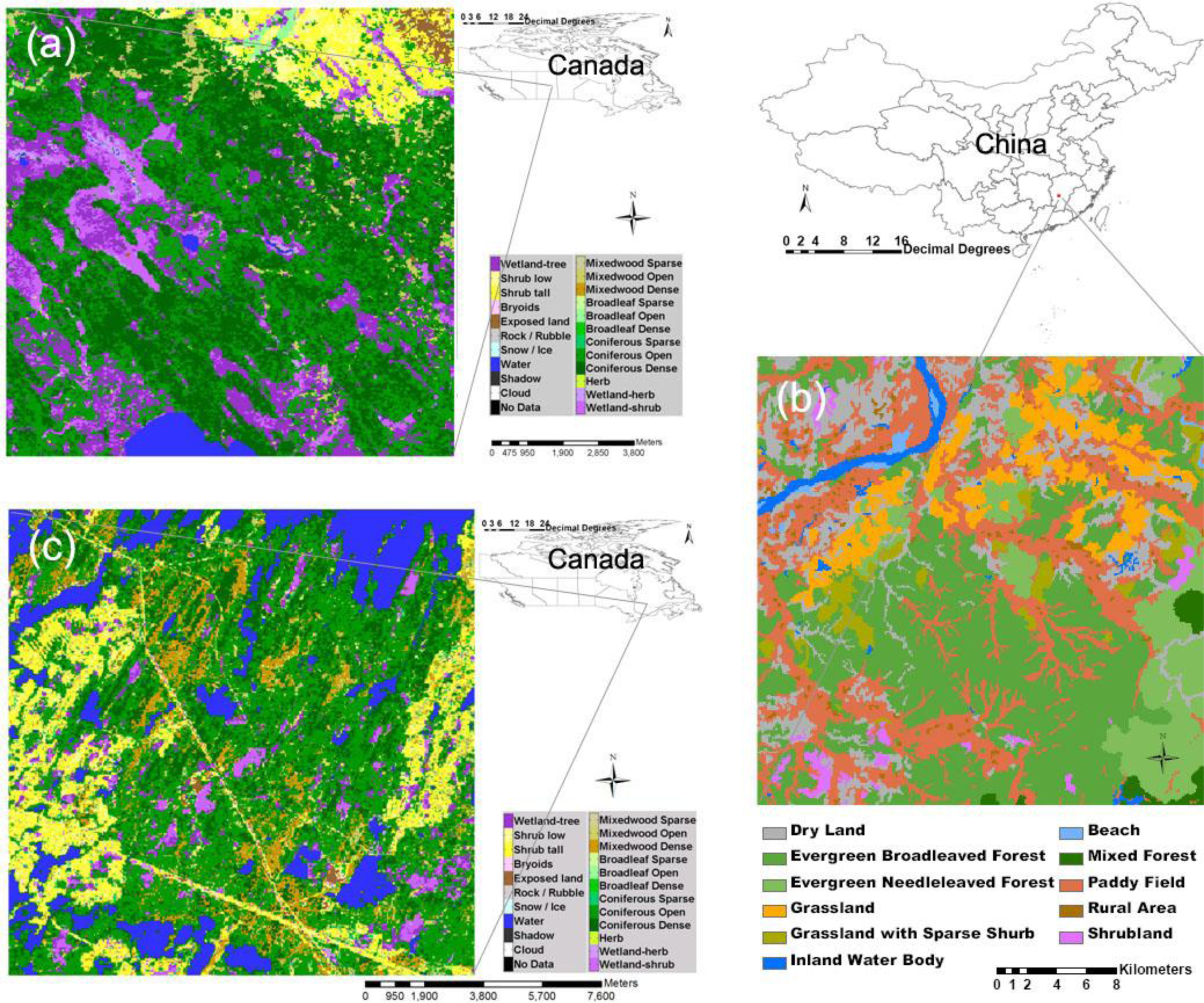
Three case study regions were selected (
Figure 1), one in China and two in Canada. The first forested study region (12 km × 12 km, 54°N, 104°W,
Figure 1a) is located near Saskatoon, Canada. This study site is characterized by rapid changes in phenology and a short growing season [
5]. The dominant vegetation is coniferous forest. The second study region (30 km × 30 km,
Figure 1b) is located in Jiangxi province, China, centered on the Qianyanzhou (QYZ) flux tower (26.74159°N, 115.05777°E), which belongs to the Chinese Ecosystem Research Network (CERN). The dominant vegetation type is coniferous forest, containing species of
Pinus massoniana,
Pinus elliottii,
Cunninghamia lanceolata and
Schima superba [
23]. The climate in this region is warm and humid, with an annual temperature of 17.9 °C and annual rainfall of 1,485 mm [
24]. The third study region (15 km × 15 km,
Figure 1c) is located in Quebec, Canada, centered on the Eastern Old Black Spruce (EOBS) flux tower (49.69247 N, 74.34204 W), which belongs to the Fluxnet Canada Research Network/Canadian Carbon Program (CCP). The vegetation in the area is dominated by a coniferous boreal forest, containing species of
Picea mariana and
Pinus banksiana [
25]. The climate in this region is warm and humid, with an annual temperature of 0 °C and annual rainfall of 1,461 mm [
26]. The time intervals for these three areas gradually increase, and the performance of the approach was tested at monthly, annual and multi-yearly time intervals.
2.2. Satellite Data and Preprocessing
Landsat TM/ETM+ data were acquired from the United States Geological Survey (USGS) EarthExplorer (
http://edcsns17.cr.usgs.gov/NewEarthExplorer/). The 8-day MODIS surface reflectance products at 500-m resolution (MOD09A1) were acquired from the National Aeronautics and Space Administration (NASA) Reverb portal (
http://reverb.echo.nasa.gov/reverb/). Only the Collection 5 MODIS data were used for the study. The data used in the study are shown in
Table 1.
Both fine- and coarse-resolution images were preprocessed before the calculation. In this study, the top atmosphere Landsat TM/ETM+ data were atmospherically corrected and converted to surface reflectance using the Landsat Ecosystem Disturbance Adaptive Processing System (LEDAPS) [
27]. Cloud and snow masking was performed using the automated cloud-cover assessment (ACCA) algorithm [
28,
29] built into LEDAPS. The atmospheric correction method in LEDAPS for Landsat TM/ETM+ data is based on the 6S model, which is also used for MODIS data [
5,
6]. The MODIS surface reflectance product data (MOD09A1) were re-projected, clipped and resampled (30 m, bilinear approach) to the same extent as Landsat TM/ETM+ data using the MODIS reprojection tools.
2.3. Land Cover Data
Two different land cover datasets were used in this study. For the study regions in Canada, we used the land cover products developed by the Canadian Forest Service and Canadian Space Agency joint project, Earth Observation for Sustainable Development of Forests (EOSD), based on Landsat 7 ETM+ data, and represents
circa year 2000 conditions. The land cover map represents 23 unique land cover classes mapped at the spatial resolution of 25 m [
30]. The accuracy of the land cover classification was found to be 77%, achieving a target accuracy of 80%, with a 90% confidence interval of 74–80% [
31]. Land cover products for the study area were acquired from the EOSD data portal (
http://www4.saforah.org/eosdlcp/nts_prov.html). For the study region in China, we used the land cover products (100 m) at the scale of 1:250,000, developed by the Earth System Scientific Data Sharing Network (ESSDSN). The qualitative accuracy of the land cover classification was found to be 80–90% [
32]. The land cover classification product in 2005 was acquired from the ESSDSN portal (
http://www.geodata.cn/Portal/metadata/viewMetadata.jsp?id=100101-11860). The land cover data were resampled to Landsat spatial resolution (30 m) using the nearest neighbor method.
2.4. Implementation of mESATRFM
We selected similar neighbor pixels according to the standard deviation and the number of land cover types within a local moving window. The number of classes was determined by land cover data. The algorithm of similar neighbor pixels selection is modified if land cover data are not available. The details are described as follows.
In the study, the land cover data were added as an auxiliary for searching for spectrally similar neighbor pixels. The algorithm of the threshold method is modified as follows. If the pixels within the local moving window of the
n-th band satisfy the following rule, they will be selected as spectrally similar neighbor pixels for the central pixel.
where
σ(
bn) is the standard deviation of the
n-th band
Bn’s reflectance within the local moving window,
s is the number of land cover types within the local moving window and
L is the land cover type. The similar neighbor pixels are selected based on the threshold of the standard deviation and under the condition that the candidate pixel has the same land cover type as the central pixel of the local moving window. The input data include two pairs of fine- and coarse-resolution images, one coarse-resolution image and land cover data. The land cover data are applied to a similar spectral pixels selection when available.
The reflectance of the central pixel (
xw/2,
yw/2) at the date of simulation,
T, can be calculated as,
where
T0 is the base date,
K is the total number of spectrally similar neighbor pixels, including the central pixel. The weighting factor,
W, and conversion coefficient
V are calculated following Zhu
et al. [
5].
According to
Equation (3), either fine-resolution reflectance at beginning date
Tb or ending date
Te can be used for calculating fine-resolution reflectance at the date of simulation,
Tp, which is marked as
Fb(
xw/2,
yw/2,
Tp,
Bn) and
Fe(
xw/2,
yw/2,
Tp,
Bn), respectively. By combining these two simulated results, the simulated central pixel’s reflectance is expected to be more accurate as the Landsat image closer to the simulated time [
6]. The temporal weighting factor is calculated as:
Thus, the final result for the simulated central pixel’s reflectance can be calculated as,
2.5. Accuracy Assessment
We assessed the accuracy of our simulations by comparing the simulated values to a Landsat observation of the same data that was set aside and not used in the simulation. A linear regression model (simulated versus observed reflectance) was used to assess the fusion models of ESTARFM and mESTARFM. RMSE (root mean squared error) is used to measure the differences between simulated reflectance values by the image fusion models (ESTARFM, mESTARFM) and the observed reflectance. MAE (mean absolute error) is a quantity used to measure how close simulated reflectance values are to the observed reflectance. R2 is used to measure the fitness of the linear regression between simulated and observed reflectance. A two-side t-test (p-value) of simulated and observed reflectance values is used to determine whether there is a statistically significant difference.
3. Results
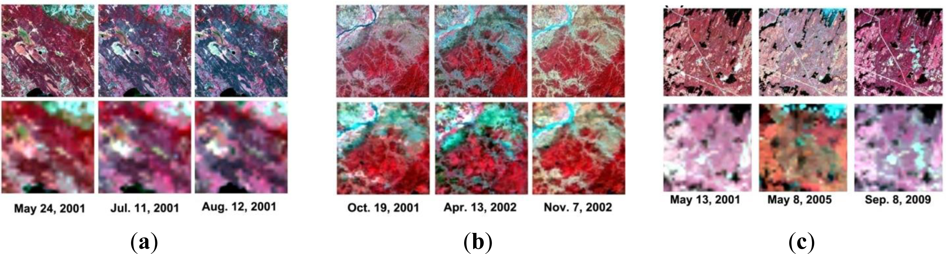
Figure 2 shows the scenes of images using NIR-red-green as red-green-blue composites for three study areas. The sub-images at the upper and lower rows are Landsat and MODIS images, respectively. The synthetic image at Landsat spatial resolution was simulated by two pairs of Landsat and MODIS imagery data and one MODIS imagery dataset at the simulated date. For example, Landsat-like imagery data (11 July 2001) can be simulated by two pairs of Landsat and MODIS imagery data acquired on 24 May and 12 August 2001, and one MODIS imagery dataset acquired on 11 July 2001. The performance can be assessed by comparing the simulated image and the observed Landsat TM/ETM+.
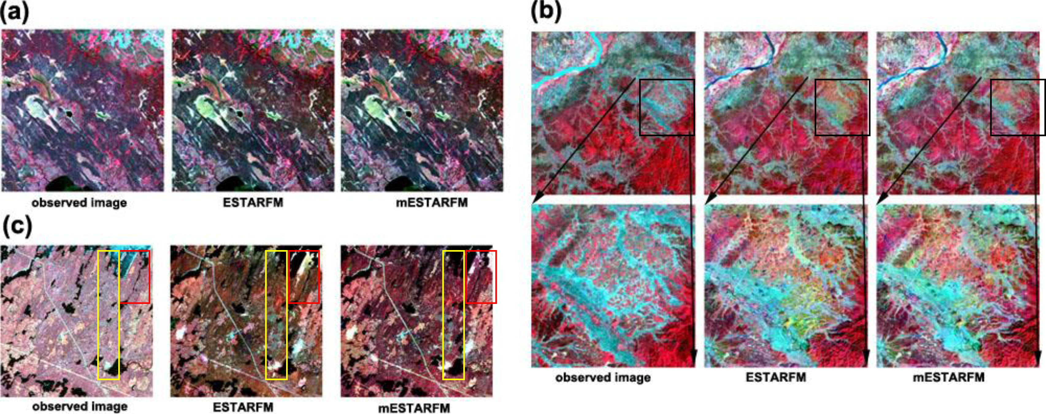
Figure 3 shows the original Landsat ETM+ and simulated images by ESTARFM and mESTARFM, respectively. For each study area, two simulated images based on two approaches were overall close to the observed image.
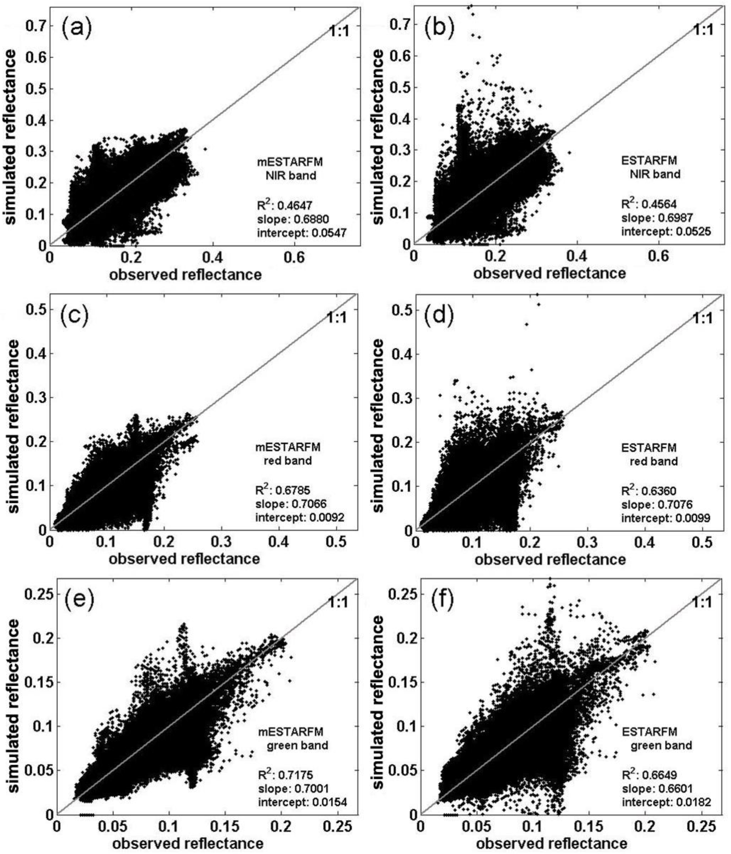
The fusion model performance was assessed by regression-based methods. For monthly changes over a forested area,
Figure 4 shows the per-pixel comparison between the simulated and observed reflectance values on 11 July 2001 for the green, red and NIR bands of Landsat ETM+. Simulated pixel values were close to the observed ones, as indicated by the 1:1 line, demonstrating that both ESTARFM and mESTARFM can capture the reflectance changes.
Table 2 (monthly changes over a forested area) shows the statistical characteristics of linear regression analysis between the simulated and observed reflectance values on a pixel basis. The simulated images for 11 July 2001 using both approaches are closer to the observed image than those for 24 May and 12 August, suggesting that the incorporated changes can be captured on the basis of MODIS images to estimate the Landsat-like image.
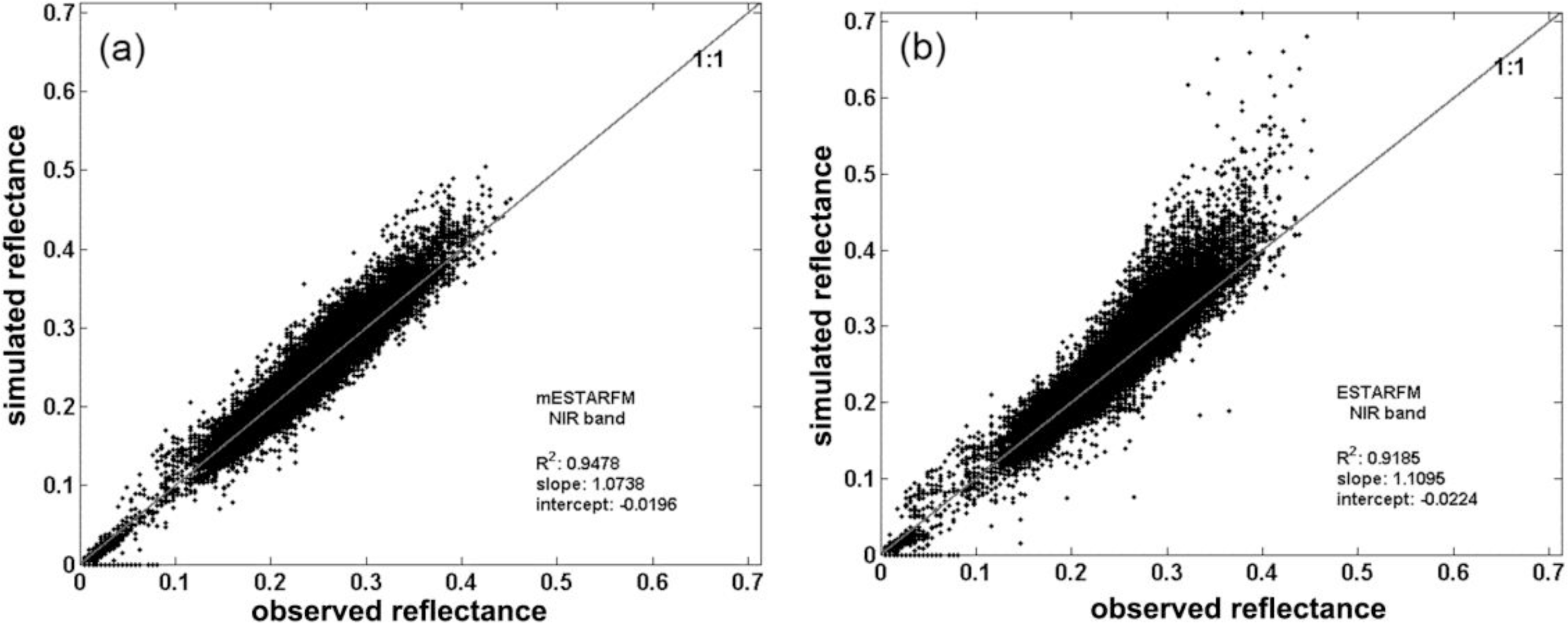
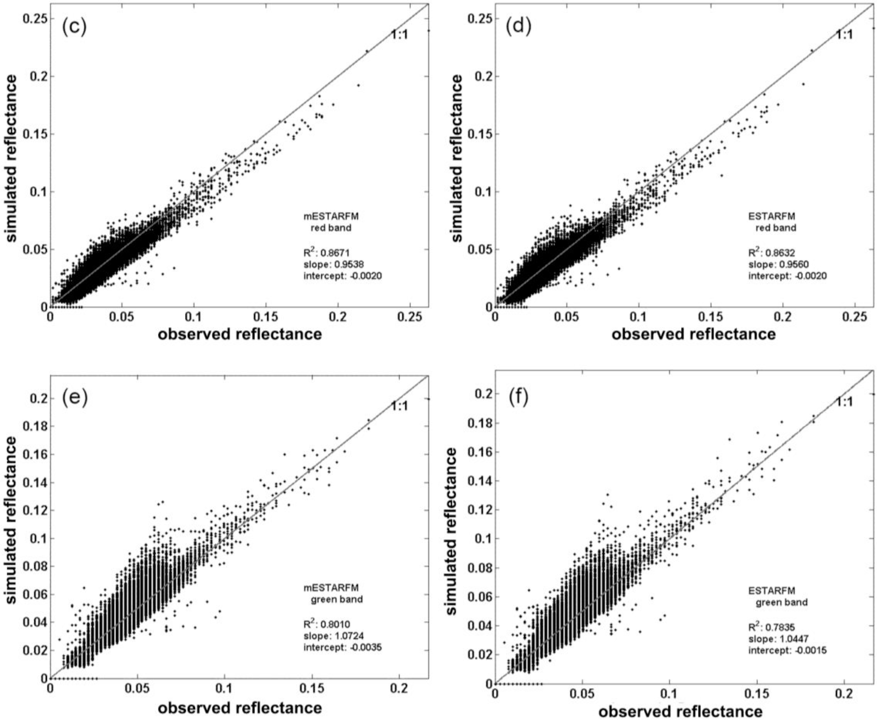
For annual changes of the heterogeneous region around the Qianyanzhou flux site,
Figure 5 shows the scatter-plots of simulated and observed reflectance values on April 13, 2002 for the NIR, red and green bands of Landsat ETM+. The rows represent the reflectance of the NIR, red and green band of Landsat ETM+, respectively (
Figure 5). The linear regression parameters (R
2, slope, intercept) are shown in
Figure 5.
Table 2 (annual changes of the heterogeneous region) shows the detailed statistical parameters of linear regression between simulated and observed reflectance for the QYZ study area.
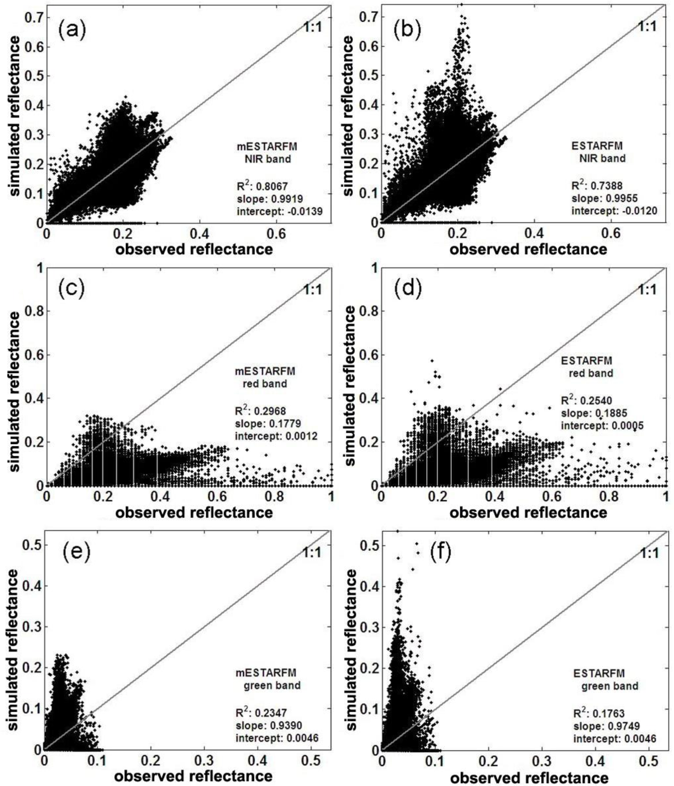
For changes of the heterogeneous region over several years around the EOBS flux site,
Figure 6 shows the original Landsat TM and simulated Landsat-like images using ESTARFM and mESTARFM. The rows represent the reflectance of the NIR, red and green band of Landsat TM, respectively.
Table 2 shows the detailed statistical parameters of the linear regression between the simulated and observed reflectance for the EOBS study area.
4. Discussions
This study introduces an updated version of the image fusion model (mESTARFM) that can blend the multi-source remotely sensed data at fine spatial resolution. The simulation capacity in the three study areas with different time intervals has been tested using the ESTARFM and mESTARFM model. Compared with the original Landsat images, the synthetic Landsat-like images produced using the updated model have higher accuracy than ESTARFM.
Specifically, mESTARFM obtains improved synthetic images, because it uses more information around the central pixel and the additional ancillary data, i.e. land cover data. As shown in the lower row of
Figure 3b, these two versions of the models have the capacity of mainly capturing the annual changes, while the updated version (mESTARFM) preserves more spatial details compared to ESTARFM. As shown in
Figures 3c and
6, for green and red bands, the performance of simulated Landsat-like images is not good. This may be caused by long time intervals and no suitable land cover data around the simulated date. This would lead to lower accuracy if any major land disturbances happened. The simulated reflectance of green and red bands contains a number of pixels with zero values, while the corresponding observed reflectance values are not, which may be due to the fact that ice only exists in the simulated date. Taking the scatter plot at three study areas into account (
Figures 4 and
6), the scatters of mESTARFM are closer to the 1:1 line. This indicates that the simulated Landsat-like reflectance results are more similar to the observed Landsat reflectance compared with ESTARFM.
The most important improvement of mESTARFM is the selection of spectrally similar neighbor pixels within a moving window with optimal size. The ESTARFM uses the information of the entire image to select the similar pixels within the local moving window; however, the information of the image is not necessarily relevant locally. According to Tobler’s First Law of Geography, the pixels that are nearer are more related to the center pixel. For the pixels outside the local moving window, the effect on the central pixel can be considered negligible. The size of the local moving window would increase until the most similar simulated fine-resolution image is obtained compared to the observed one. Besides this, the land cover data were used as auxiliary information for the selection of spectrally similar neighbor pixels. The criteria for determining spectrally similar neighbor pixels includes the threshold of standard deviation, the number of land cover types and the difference between the central pixel and neighbor pixels within the local moving window.
Although improvements of mESTARFM are made, there are still limitations, including: (i) the available land cover data for a certain date may not be sufficient for the spectrally similar neighbor pixels, since that land cover type may change from date 1 to date 2; (ii) the land cover data may not take much effect if the date suitable for the land cover data is far away from the simulated time. Therefore, further research may need to focus on the following issues: (i) The combination of the land cover classification data on date 1 (beginning) and date 2 (ending); the pixels may obtain whether land cover type changes between these two dates [
20]. More accurate remotely-sensed data can be simulated if more accurate similar neighbor pixels are selected according to the better classification algorithm. (ii) The establishment of the typical vegetation’s annual variation of spectral reflectance curve may be useful to get more accurate conversion coefficients. (iii) A combined Spatial Temporal Adaptive Algorithm for mapping Reflectance Change (STAARCH) [
15]/mESTARFM approach could better indicate the disturbance or changes in spectral reflectance, and that would improve the predictions.


