1. Introduction
Disaster preparedness and mitigation require accurate information about buildings and other infrastructure that might be impacted by a typhoon, earthquake, or other disaster. For example, Kyoto, the ancient capital of Japan, is a UNESCO World Heritage site with hundreds of irreplaceable structures, many of which are wooden. The active Hanaore fault lies under downtown Kyoto. If an earthquake occurs, fire may spread through dense urban areas and the valuable historical structures, located in the dense urban areas, would be burnt and lost. Architects and engineering researchers have attempted to simulate the damage caused by fire to support evacuation planning and other disaster prevention measures. A physics-based fire spread model has been developed [
1], and its performance examined by application to the dense urban areas of Kyoto [
2]. Such models require many building parameters including three-dimensional (3D) building models. However, 3D building models are not available to researchers at a reasonable cost. Google Earth provides 3D building models, but its models of the Higashiyama area are poor because dozens of Japanese houses are modeled as a single box model. Better simulation of fire spread requires a model that separates individual buildings [
1].
Airborne light detection and ranging (LiDAR) can provide the data necessary for generating three-dimensional models. 3D building modeling using airborne LiDAR has been studied for more than a decade, and existing algorithms have produced both simple models [
3–
4] and more detailed models [
5–
7]. Building modeling is principally based on the segmentation of point clouds into a number of point groups that correspond to each building. The degree of detail in the model depends on the requirements of the model and the density of the LiDAR data. The point groups obtained during the process are used in the model to represent the shape, height, and spatial arrangement of the real buildings. This method assumes that the original LiDAR point clouds can be classified into small groups of points that reflect the individual buildings.
Automatic 3D building modeling in dense urban areas is a well-known challenge. For example, in dense urban areas in Kyoto, Japan, traditional Japanese houses are located close to each other, and the heights of the ridges on the roofs are similar. Modeling of buildings in some urban areas might be possible using current techniques, even if the buildings are located close to one another, as their heights are often dissimilar and differences in height can be easily detected. In contrast, houses having similar heights might be difficult to model using existing algorithms because the point cloud cannot be separated into groups representing individual houses based on height information alone.
To improve modeling accuracy, some researchers have examined fusion of airborne LiDAR data with a digital map [
8]. As such approaches require a pre-existing digital building map, they might be costly to apply to large urban areas. As alternatives to digital maps, other data sources have been examined, such as aerial or satellite images [
9–
13] and terrestrial LiDAR data [
14]. In particular, aerial images are promising for providing data showing individual buildings in dense urban areas. Existing research shows that a key aspect of efficient data fusion in 3D modeling is obtaining building geolocation and shape information from 2D images, in addition to obtaining 3D coordinate data from airborne LiDAR data. However, to the author’s knowledge, even when combining data sources, no successful modeling algorithm has been reported that can be applied to an area where houses of similar height are located close to one another. The main reason for this shortcoming may be due to the difficulty in segmentation of buildings located close to each other from images.
Object-based segmentation is a conventional approach for extracting building geolocation and shape information from images. This segmentation technique is widely used in a number of applications, including the mapping of urban areas [
15–
17]. However, in our previous research [
18], object-based segmentation using commercial software (ENVI EX Version 4.8) produced poor results when tested on an image of dense urban areas with spatial resolution of 25 cm. Factors in the unsuccessful segmentation were as follows: (1) unclear building boundaries caused by roofs with similar brightness being located close to each other; (2) shadows cast by neighboring buildings; and (3) roofs having a rough texture. Our paper cited above proposed an algorithm that considers these factors and that can effectively segment buildings, including shadowed buildings, in dense urban areas through the use of aerial images.
In the current paper, another algorithm is proposed for automatic generation of 3D building models for dense urban areas, by using the building segmentation results from aerial images produced by the aforementioned algorithm in combination with airborne LiDAR data. In addition to information about the building area, normals to the roofs are determined for groups of buildings that are linearly aligned. By taking account of the segmented regions and the normals, the method selects the correct building roof types and generates models that are more accurate than those produced by previous methods.
The remainder of this paper is organized as follows. An overview of our previously reported segmentation algorithm is given in Section 2, along with an explanation of the newly proposed method. The locations used in the study, and the data collected from these sites are described, and the experimental results are reported in Section 3. The implications of these results and the validity of the algorithm are then discussed in Section 4. Finally, Section 5 concludes the paper.
2. Methodology
The proposed algorithm for automatically generating 3D building models consists of three parts: (1) image segmentation, (2) LiDAR data filtering, and (3) 3D building modeling.
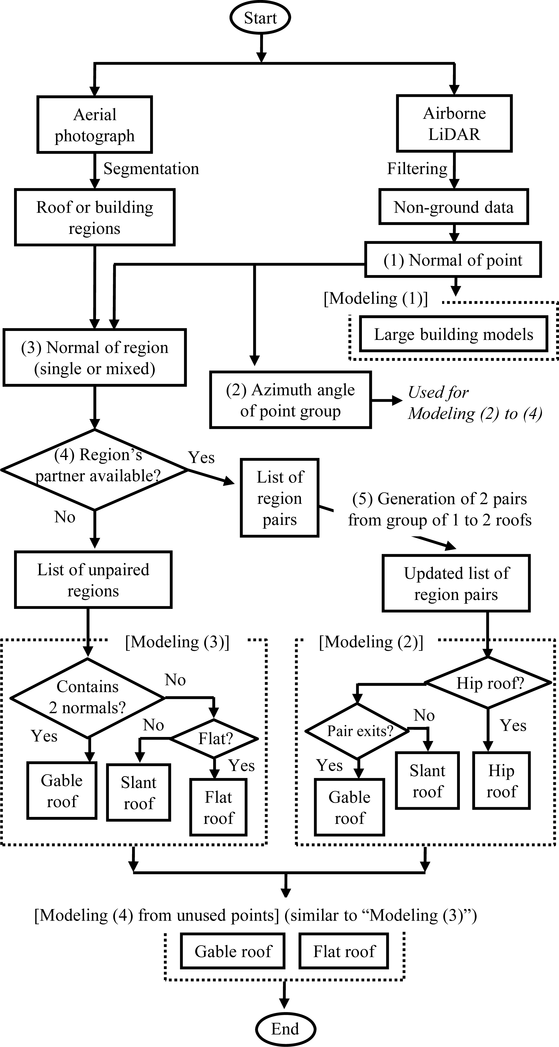
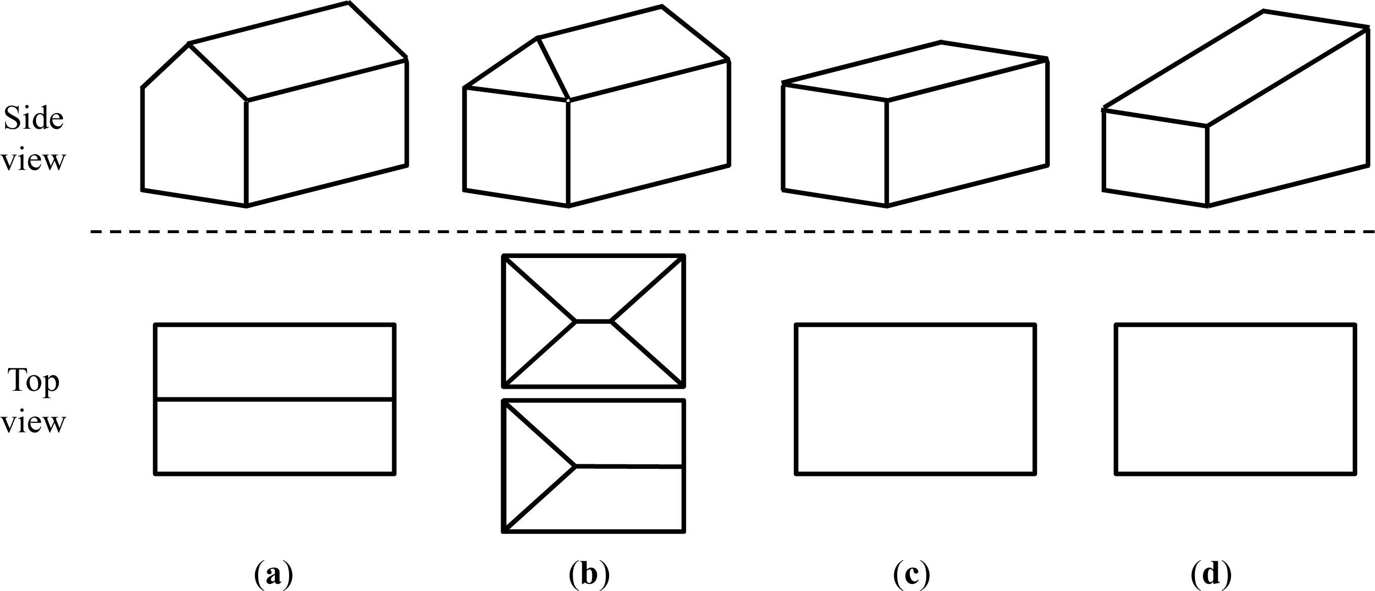
Figure 1 shows a flowchart of the algorithm. The algorithm assumes four simple building types: gable-roof, hip-roof, flat-roof, and slant-roof buildings. Two types of hip-roofs are included: two-sided and one-sided (
Figure 2). The segmentation algorithm [
18] and filtering algorithm [
19] used in the current work have been described elsewhere, and the details of the algorithms are omitted in this paper.
The 3D building-modeling algorithm introduced here first calculates region normals to generate models that are orderly arranged in dense urban areas. Then, incomplete segmented results are improved before modeling. Finally, the algorithm generates 3D models under four modeling strategies. In cases where models generated overlap each other, model boundaries are corrected. The details of the algorithm are described in the following subsections.
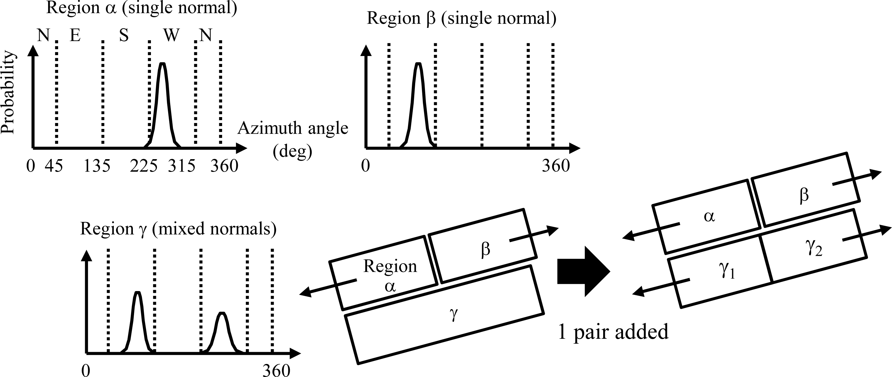
2.1. Calculation of Region Normals
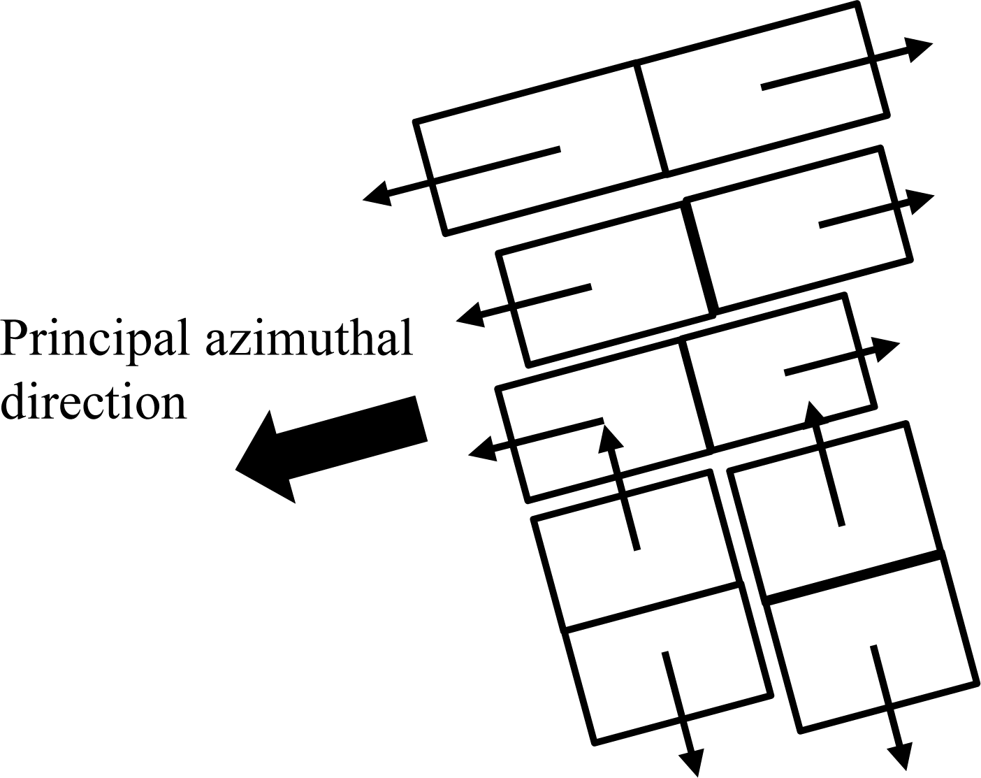
In preliminary modeling of buildings in dense urban areas, we observed that the azimuthal direction of the roof normal is important to generate models in dense urban areas. However, if normals are estimated on a per-building basis, the spatial arrangement of generated building models will be independent, and then they will be difficult to keep in a line, a common pattern found in dense urban areas. The proposed algorithm for generating 3D building models focuses on the geospatial arrangement of buildings in dense urban areas. Principal azimuthal directions of roofs are estimated based on building groups and utilized for determining individual roof normals (
Figure 3).
In Step (1), the algorithm calculates the normal of each LiDAR point using neighboring points within a window (Parameters (a) and (b) of
Table 1) by fitting a plane. If the root mean square error (RMSE) is below a threshold (Parameter (c)), the obtained normal is used for all points within the window. Here, the vertical component of the normal (
nx,
ny,
nz) is defined as
nz, where
. If the vertical component of the normal is greater than another threshold (Parameter (d)), the normal is labeled as a “vertical normal”; otherwise, the normal is labeled with a direction (north, south, east, or west).
Step (2) segments the point clouds into groups on a building-block basis by examining the horizontal and vertical distances to each point’s nearest neighbors. If these distances are less than the respective thresholds (Parameters (e) and (f)) the point is added to the building block containing the neighbor. Each group of points that form a building block is allocated a principal azimuthal direction by finding the peak of the probability distribution generated from the normals to the points (
Figure 4). The definition of the probability is the ratio between the frequency of a specific angle (degree) and the sum within the building block of frequencies in all angles (360 degrees). These azimuthal directions are used in Modeling (2) to (4).
2.3. Multi-Strategy Modeling
The proposed algorithm includes four modeling strategies. First, Modeling (1) is conducted after Step (1), with the aim of modeling relatively large flat-roof buildings. In segmenting the aerial image, we found that commercial buildings, parking structures, and other flat-roof buildings were often segmented into small areas because of objects on the roof, making it inappropriate to model such buildings using the segmented results. Therefore, Modeling (1) is conducted using only the LiDAR data without the segmented results. Point clouds are segmented by setting vertical and horizontal distance thresholds (Parameter (m)). Point clouds having a certain number of points (Parameter (n)), and whose dominant normal class is “vertical”, are used to generate large flat-roof building models.
As a result of improving incomplete information, two lists are generated: a list of region pairs, and a list of regions without pairs. Modeling (2) uses the first list. It generates models for those regions whose normals are not vertical and whose partners are available, in descending order of each region’s area. A point shared by two regions is determined to be a point on a ridgeline. If no point is shared by two regions, a centroid of edges of the two regions is used as an alternative. The ridge direction is established such that it is orthogonal to the azimuthal direction of the two regions’ normals. A search is conducted, on both sides along the ridge direction, for regions whose normal azimuthal direction is parallel to the ridge’s direction. If two such regions are detected, a two-sided hip-roof building model is generated. If one such region is detected, a single-sided hip-roof building model is generated. If no such region is detected, a gable-roof building model is generated. During this modeling process, the minimum length of the rectangle (Parameter (o)) and minimum area (Parameter (p)) are checked to exclude small models that are probably artifacts.
Using the list of regions without pairs, Modeling (3) generates models for the regions remaining after Modeling (2). If a region has a mixed normal class and its two azimuthal directions are linearly symmetric (e.g., Region γ in
Figure 4), a gable-roof building model is generated. If the region has a single slanted normal, a slant-roof building model is generated. Otherwise, a flat-roof building model is generated.
After Modeling (3), some points may remain unused because they did not meet the criteria for strategies (1) through (3). In addition, there may be inconsistencies between the LiDAR data and aerial image observations. When a building does not exist in the aerial image, but does exist in the LiDAR data, the area of the building will not be segmented. In this case also, the points of the building area will remain unused. Modeling (4) generates models using the unused points. Similarly to Modeling (3), additional gable-roof or flat-roof building models are generated based on the azimuthal direction. If some points still remain unused after this process, flat-roof building models are generated without using the azimuthal direction (Parameters (m) and (n)). Because points used in Modeling (4) may include points reflected from tall vegetation, vegetation removal should be executed before modeling. This issue will be discussed in Section 4.1.
2.4. Determination and Correction of Model Boundaries
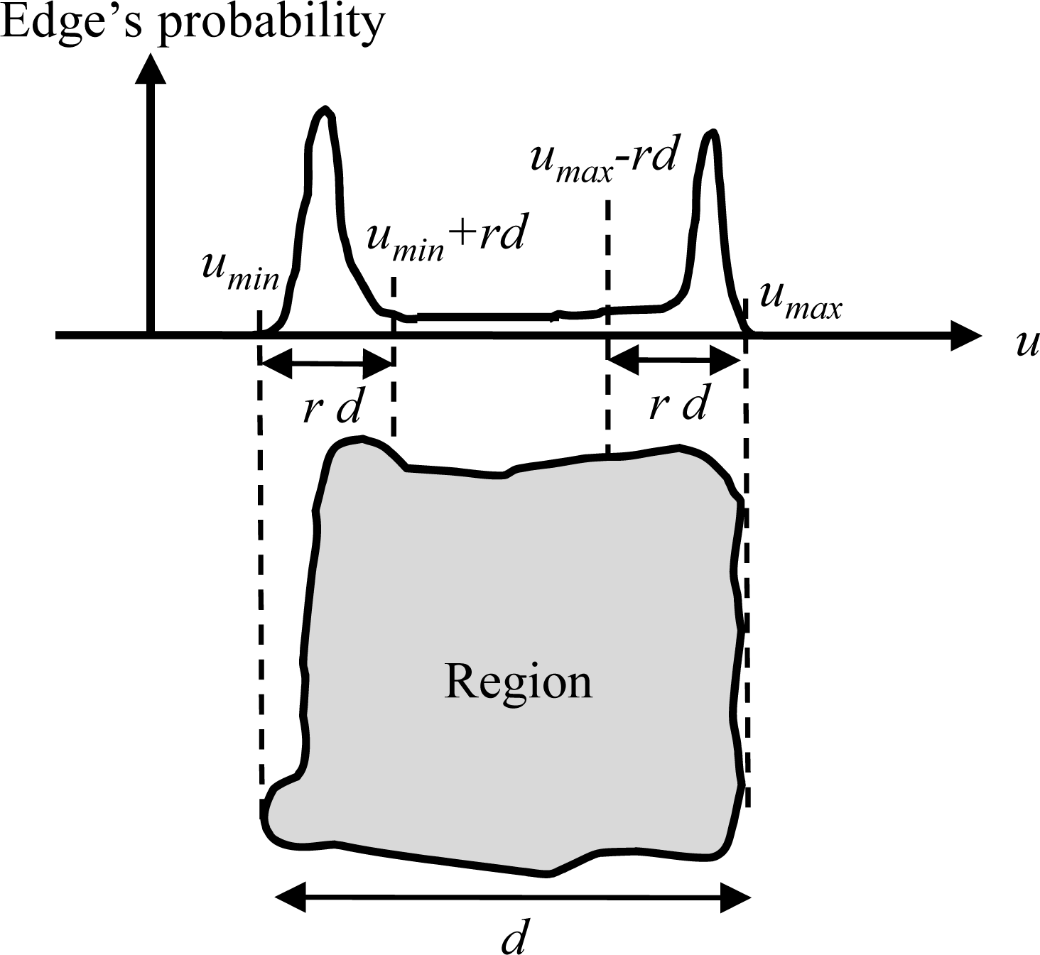
In the proposed algorithm, the boundaries of each building are assumed to be orthogonal or parallel to the principal azimuthal direction of its associated group of buildings. That is, buildings are assumed to be rectangular. The boundaries of a modeled building are generated such that their directions are parallel or orthogonal to the principal azimuthal direction of the building-group point cloud in which the model is included. In actuality, a model's geolocation is highly dependent on the regions segmented using the aerial image. Because geolocational and sizing errors could be included in the segmented regions, a number of corrections are performed, as shown in
Figure 6. We determine the “true” location of an edge by doing a local search and evaluating edges along the principal direction of a region and the orthogonal direction. Edges of segmented regions from aerial image are projected onto the principal azimuthal direction of a region (called the “u-axis”), and the probability density is generated. The definition of the probability
P(
u) is:
where
n(
u) denotes edge frequency at a specific
u and
N denotes the total number of edges in the region. The width
d of the region along the
u-axis is defined as:
where
umax and
umin denote the maximum and minimum
u values, respectively. The maximum probability is searched for within an interval of width
d multiplied by a prescribed ratio
r (Parameter (l)), that is, [
umin,
umin +
rd] and [
umax –
rd,
umax] for lower and upper boundary detections, respectively. The
u value that occurs with highest probability among the two intervals is selected as the boundary location. The same process is repeated along an axis orthogonal to the principal direction (called the “v-axis”).
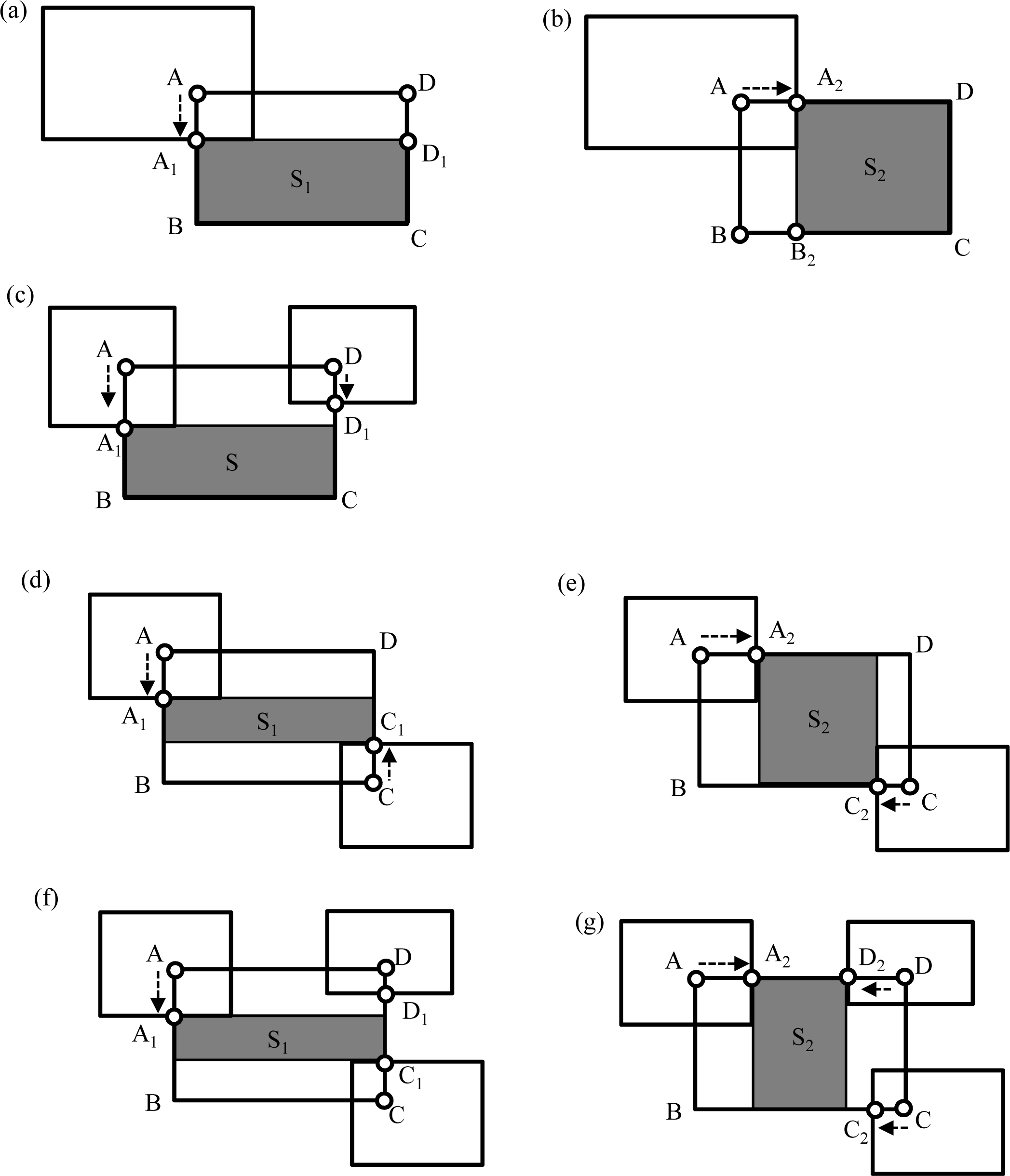
If a generated model overlaps an existing model, the boundary of the model is corrected by implementing the following process. If one vertex of a rectangle overlaps the area of another modeled building, as shown in
Figure 7a,b, the overlapping vertex (Point A) is shifted in two directions (toward Points A
1 and A
2) along the rectangle’s sides. Accordingly, the sides connected to the vertex are also shifted (AD to A
1D
1 and AB to A
2B
2). The shifted vertex is selected on the model whose rectangular area, S
1 or S
2, is the greater.
If two adjacent vertices overlap another building, as shown in
Figure 7c, the side between the vertices is shifted to avoid overlapping. In
Figure 7c, lengths A
1B and CD
1 are compared and the shorter is selected for relocating the side. If two diagonal vertices overlap, as shown in
Figure 7d,e, a procedure similar to that for single vertex overlapping is performed. The shifted vertices are selected on the model whose rectangular area, S
1 or S
2, is the greater. If three vertices overlap, as shown in
Figure 7f,g, a procedure is executed that combines the procedures for two adjacent and two diagonal vertices overlapping. The shifted vertices are again selected on the model whose rectangular area, S
1 or S
2, is the greater.
4. Discussion
4.1. Effect of Segmentation Quality on Modeling
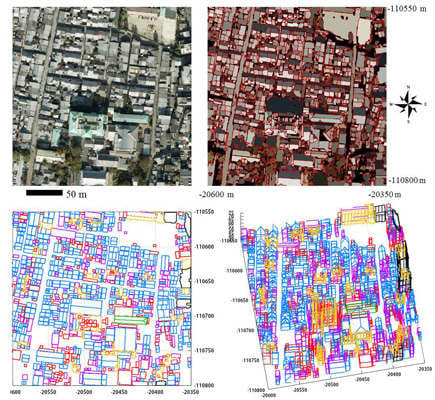
The proposed algorithm can generate different types of building models, and generated almost the same number of models as actual buildings in the study area. The primary factor in realizing a successful model is appropriate utilization of the region areas provided by the segmentation from aerial images. The primary factor in realizing a successful model is making the best use of the region areas provided by segmentation of aerial images.
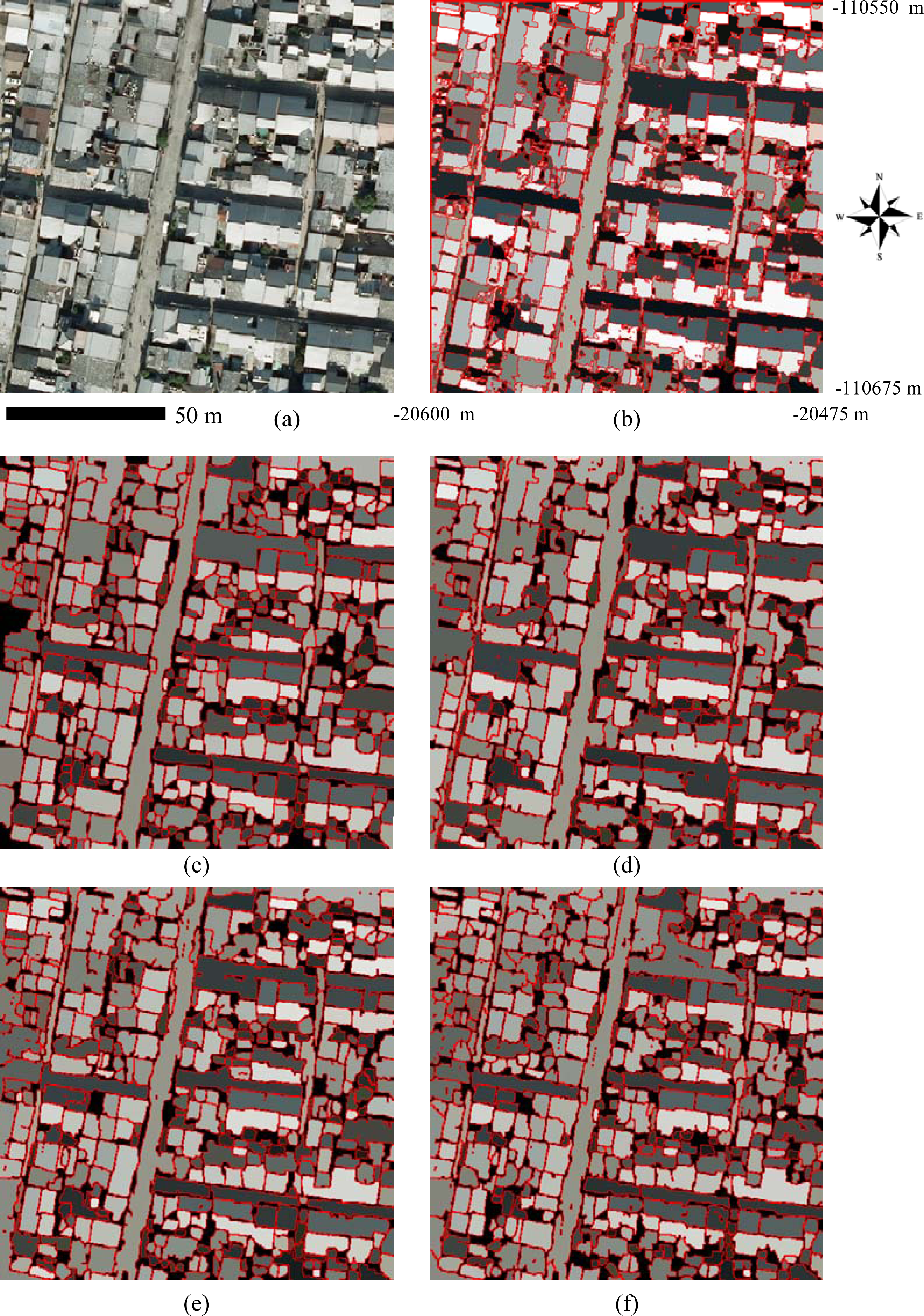
Figure 14 shows the segmentation results for the upper left area of
Figure 12a. The final result (
Figure 14c) was generated by selecting regions with higher rectangular index from the regions generated under different discrete widths (
Figures 14d–f)). This result shows that the segmentation algorithm [
18] outperforms ENVI EX [
20] (
Figure 14b), and that the segmentation algorithm selects optimal rectangular regions. This indicates that the algorithm can find the optical local smoothing parameter for segmentation. However, the segmentation algorithm has room for improvement, since it failed to exclude road surfaces, and sometimes failed to separate individual roofs. To improve these results, road surfaces were subsequently excluded by counting the effective points that were significantly higher than the ground elevation estimated through filtering.
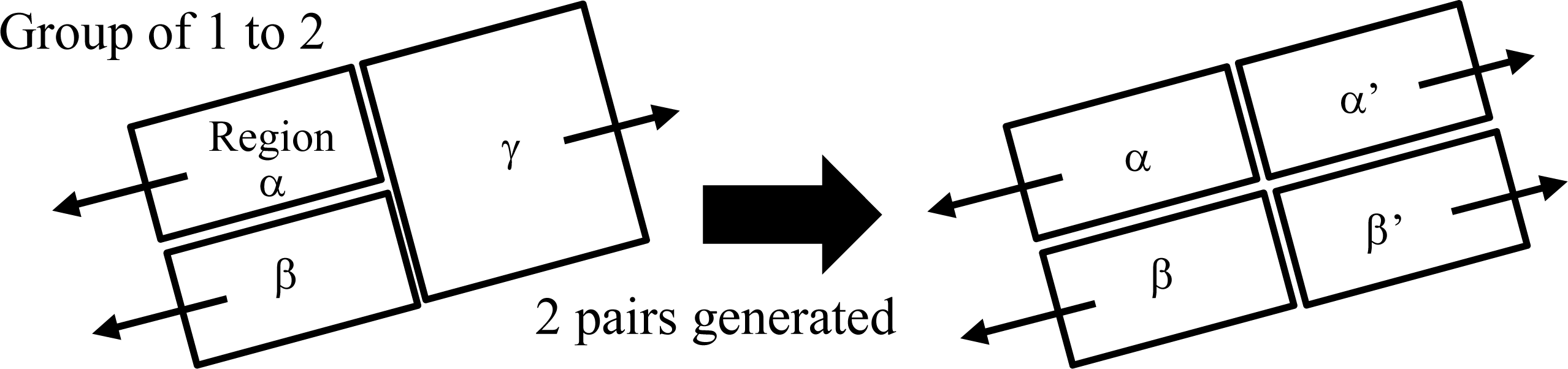
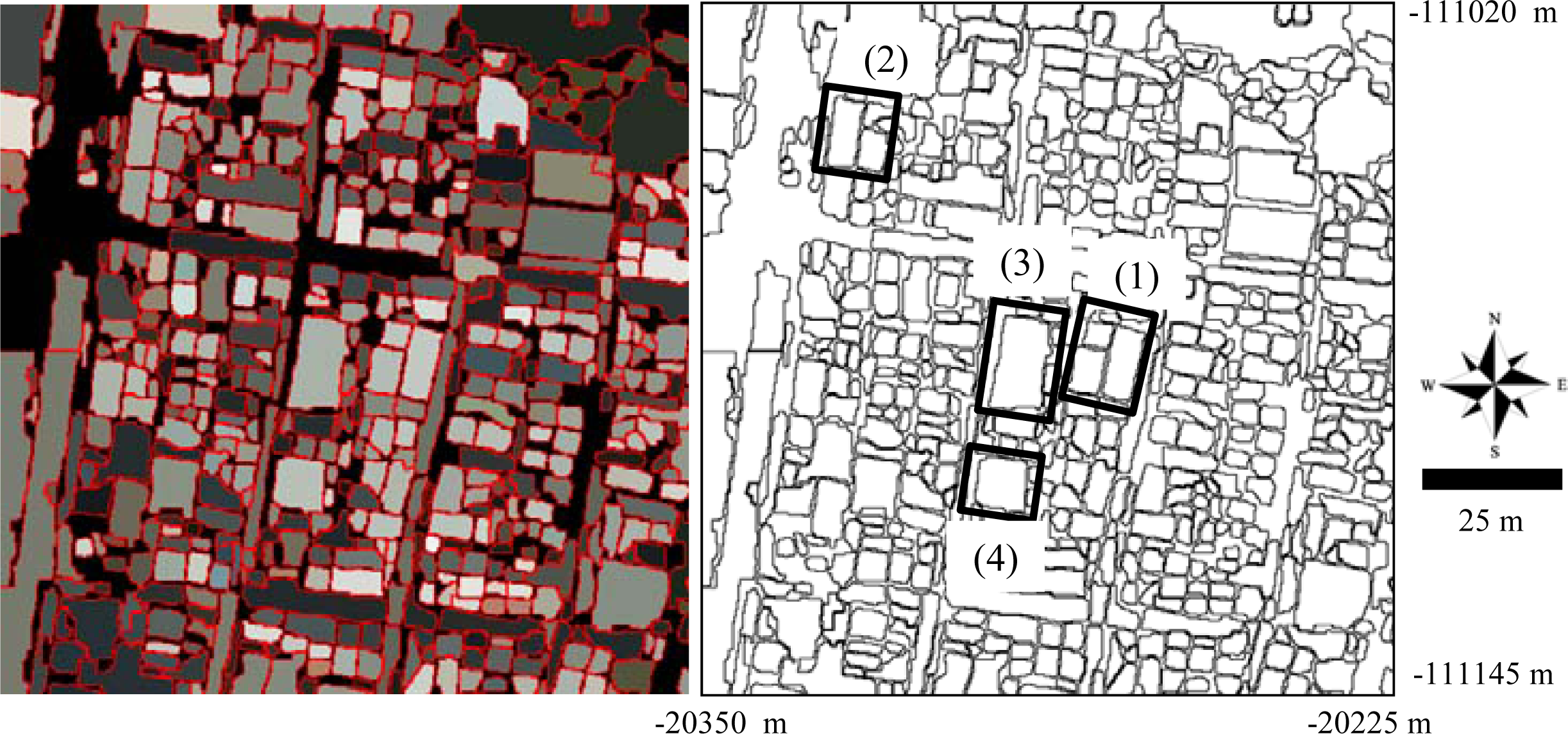
For the case of failing to separate two-roof regions, later steps in the proposed algorithm generate a gable-roof building model if the regions possess two normals that are linearly symmetric, and generate two pairs of gable roofs when groups of 1 to 2 roofs are found in the segmentation results. By employing these knowledge-based approaches, the proposed algorithm utilizes the geometry of the buildings for modeling, reducing the impact of segmentation errors. Columns (b) and (c) for the gable-roof buildings in
Table 4 show that despite segmentation errors, modeling of these buildings was successful. For example, Areas (1) and (2) in
Figure 9 show generated models when groups of 1 to 2 roofs were found in the segmentation results, and Areas (3) and (4) show generated models when regions possessed two normals that were linearly symmetric.
Although the segmentation information from aerial images is important, buildings whose regions are not extracted in segmentation can still be modeled in the proposed algorithm. Modeling (4) generates models by using point clouds that are not currently in use in the model, but that indicate that a building most likely exists.
Figure 10e shows that the proposed algorithm succeeds in modeling some missing buildings and compensates for segmentation failure. As points used in Modeling (4) may include points reflected from tall vegetation, vegetation removal is executed before modeling. An examination of the areas revealed that in estimating the coefficients for the planar equation, some point clouds reflected from tall trees had small RMSEs. Therefore, the brightness of aerial images could be utilized to avoid generating false models. However, it was difficult to exclude vegetation because of color variety (green, yellow, or red) and crown shadows. Manual removal of vegetation may be painstaking if vegetation areas are not small. In such cases, semi-automatic removal may be reasonable by setting combinations of RGB DN thresholds for green, yellow, and red vegetation, respectively. Techniques for removing vegetation should be improved in the future.
The compensatory factors built into the algorithm also help reduce the effects of the difference in time between the acquisition of LiDAR data and aerial image observations. Whether the image was taken before or after LiDAR observations, certain buildings that exist in the aerial image may not have been captured by LiDAR. Such buildings are removed from the modeling process by our LiDAR filtering (because at the time of LiDAR acquisition, they are in fact ground points). In contrast, if buildings observed by LiDAR are not segmented due to segmentation failure, or are not available in the aerial image due to demolition or construction, these buildings can still be modeled by performing Modeling (4). Therefore, effects due to observation delays can be reduced, and the proposed algorithm can generate models for all buildings available when the LiDAR data are acquired.
A number of point clouds remained even after Step (8) had generated models. Yellow areas in
Figure 10d shows that these point clouds correspond to building roof sections. We explored a provisional technique that merged such point clouds with the generated models. However, classification of points into the models was unstable. Therefore, at this moment, a semi-automatic approach to correcting models is reasonable, and a fully automatic approach will be further examined in the future.
4.2. Accuracy Assessment
Table 3 shows that the producer’s accuracies for gable-roof, flat-roof, and slant-roof buildings were all within acceptable limits for the models required for a fire spread simulation, whereas the hip-roof producer’s accuracy was not acceptable.
Table 4 records the conditional probability of generating a building model, given that the building areas are correctly segmented. Flat-roof models generated in Modeling (1) were excluded from
Table 4 because they were modeled without using the segmented image. Columns (b) and (c) for the gable-roof show that modeling of gable-roof buildings was successful even when not supported by segmentation results. However, column (a) of the hip-roof results shows that modeling of hip-roof buildings was difficult even with completely successful segmentation. In the unsuccessful cases, the side roof planes of the buildings had a low number of LiDAR points and were not of a single normal type. As a result, the side roof was not regarded as a part of the hip-roof building. Especially in dense urban areas, small roofs may not contain enough data points to calculate their normal, owing to occlusion. The results also show that smaller hip-roof buildings may not be correctly modeled because of the incident angle of the LiDAR; however, this problem can be overcome if higher density airborne LiDAR data is made available for the modeling.
Table 5 shows that the proposed algorithm underestimated the total ground area of the models by 14.0%. When segmenting regions from aerial images in dense urban areas, accurate delineation of building boundaries is a nontrivial problem. Our method corrected the boundaries to eliminate overlapping buildings, as shown in
Figure 7. However, this strategy for dealing with overlap generally reduced the area of the overlapping buildings. As a result, the ground areas of models are expected to be underestimated for dense urban areas.
4.3. Variety of Generated Models
The proposed algorithm generates four types of building models: hip-roof, gable-roof, flat-roof, and slant-roof; each has a rectangular rooftop. Some users may not be satisfied with these simple models, especially because more comprehensive model sets have been generated by other research groups [
5–
7]. However, as mentioned in Section 1, the aim of the present research is to generate models of dense urban areas, for which the algorithms for automatic modeling have been inadequate. The proposed approach overcomes the difficulty of modeling dense urban areas by referring to the regions provided by segmentation from aerial images.
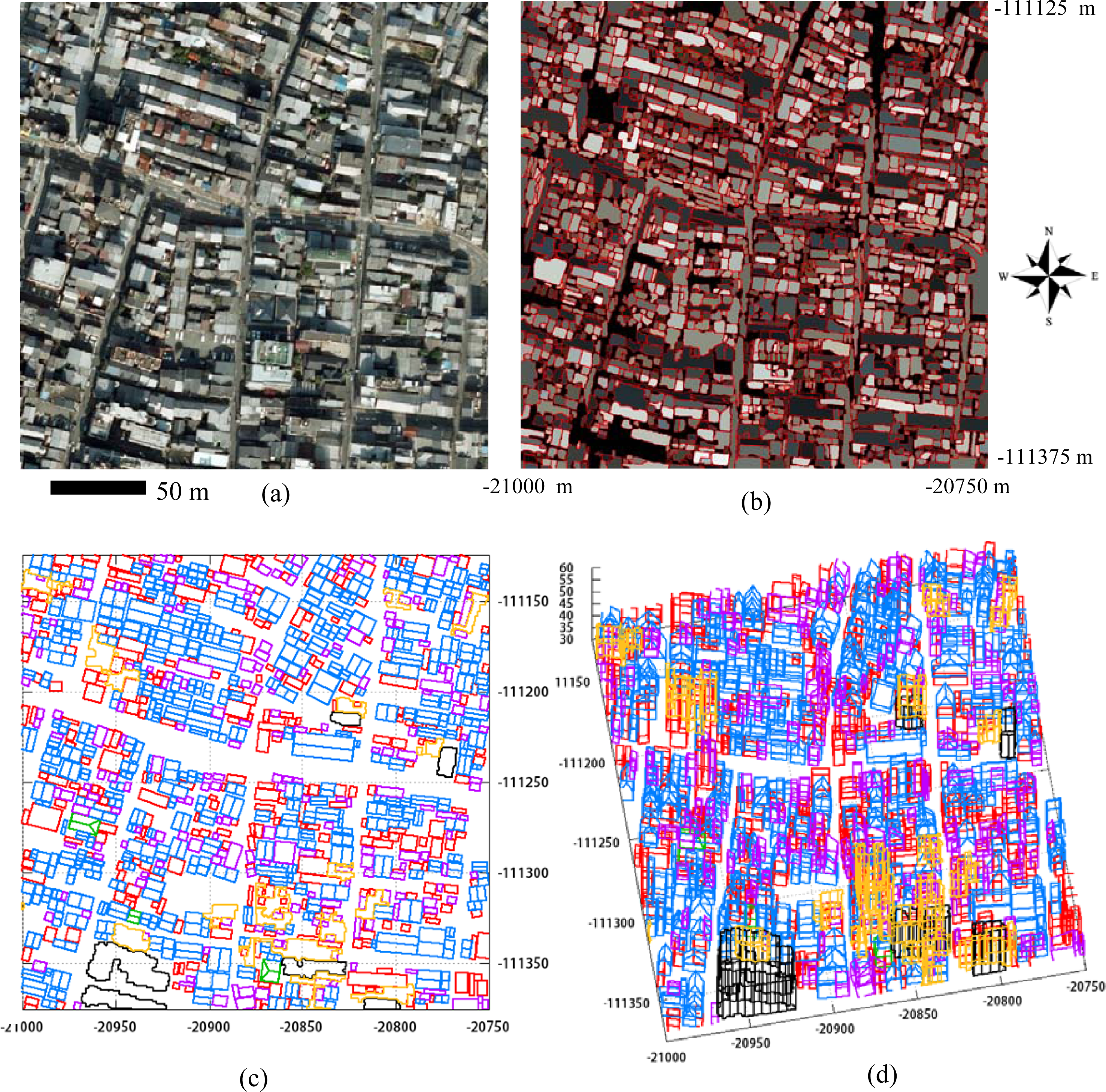
The proposed algorithm modeled complex buildings as one of the four models, a combination of the four models, or a model with some missing parts. For example, L-shaped gable-roof buildings (Area (1) in
Figure 11a) were modeled by gable-roof and flat-roof building models in
Figure 11c,d. In the area containing low-rise buildings and high-rise and complex buildings, the complex building (Area (1) in
Figure 12b) was modeled as a large gable-roof model, and other complex buildings in the area were properly modeled as gable-roof models.
For Kyoto, simple models, rather than detailed models, have been requested by researchers in the field of disaster assessment for modeling the propagation of fire caused by an earthquake. In terms of feasibility, it remains difficult to automatically generate detailed models of dense urban areas, even by combining high-density LiDAR data and aerial images. As a result, the author generated simple models rather than complex models. If users wish to generate detailed models or models with non-rectangular rooftops, it is recommended to determine whether the boundary of the building is nearly rectangular by examining the shape of the segmented region. If it is not nearly rectangular, another model with a non-rectangular rooftop should be applied.
4.4. Determination of Azimuthal Direction of Ridges in Dense Urban Areas
In developing the algorithm, we found that the roof and the ridge directions of buildings aligned in a row tended to be inconsistent when the directions were estimated individually for each building. This misalignment was due in part to the low density of the airborne LiDAR data and in part to the inaccurate separation of points from different roofs or different buildings, as a consequence of incomplete segmentation. To reduce the effects of this inconsistency, a method was implemented, where filtered point clouds were separated into small groups, and the principal azimuthal direction of all the points in a group was used to determine the roof and the ridge directions, and also the boundaries of the buildings. As a result, accurate models of rows of buildings in dense urban areas were generated even when using the low-density airborne LiDAR data.
The restriction of azimuthal roof alignment is useful to apply the proposed algorithm to dense urban areas, where alignments are generally consistent. Note that this approach might not work for a building whose roof’s azimuthal direction is completely contradictory with those of other buildings. However, as shown in
Figures 11 and
12, such conflicting buildings were not observed in any of the study areas. If a building with a different azimuthal direction exists a few meters away from other buildings, the point clouds associated with that building can be easily separated from the other point clouds, and thus the roof and the ridge directions are accurately estimated. In this regard, in the case of non-dense urban areas where buildings are not close to each other, the algorithm still works because the roof and ridge directions are determined within point clouds classified using Parameter (e), horizontal and vertical distance for segmentation of point clouds. The argument here is that determining a building’s azimuthal direction is highly dependent on point clouds being separated building by building, as mentioned in Section 1. Because this separation is difficult for dense urban areas, the approach taken in the proposed algorithm is reasonable.
4.5. Parameter Selection
The parameter-setting process and the sensitivity of the results to the parameter selections are important in terms of transferability of the proposed algorithm. The factors affecting the parameters can be classified as follows: (1) artificial geographical features (e.g. average building area/size, and street width); (2) LiDAR point density; (3) both artificial geographical features and LiDAR point density; and (4) others. Factor (1) is dependent on the study area, and impacts the following parameters: (e) horizontal and vertical distance for segmentation of point clouds, (f) minimum height for discrimination of roof points, (k) minimum ratio between maximum length of the smaller region and that of the larger region, (m) horizontal and vertical distance for segmentation of point clouds, (o) minimum length of rectangle, and (p) minimum area. Factor (2) impacts parameter (a) window size. Parameters affected by Factor (3) are as follows: (d) minimum vertical component of normal for flat roof, (g) minimum probability for single normal class, (h) minimum probability for two normal classes, and (n) minimum number of points. Parameters (i) minimum valid length, (j) maximum invalid length, and (l) ratio r for boundary search can be determined by the quality of the segmentation result of aerial image, and its spatial resolution.
In case of the study area, it took 20 to 30 iterations to check the validity of the selected parameters. In particular, the values of Parameters (g) minimum probability for single normal class and (h) minimum probability for normal classes were found to be very sensitive. As it may be difficult to automatically optimize such parameters, empirical optimization may be necessary. If the proposed algorithm is to be applied elsewhere, it will need to use different parameter values. In particular, application to non-dense urban areas may need to tune parameters included in Factors (1) and (3).
4.6. Computation Time
It took approximately 10 min of elapsed time to model one study area (250 m × 250 m); 5 min 30 s for filtering (approximately 1 km × 1 km), 4 min for segmentation using an aerial image (250 m × 250 m), and 1 min 20 s for modeling using filtered LiDAR data and a segmented image (250 m × 250 m). Most of the computation time is spent segmenting the aerial image. Based on this result, it should take approximately 26 min to model a 1 km × 1 km area. The modeling results may require manual corrections. However, even when including the time for manual corrections, it should be possible to model a 1 km × 1 km area within an hour. This should be an acceptable amount of effort for researchers simulating fire spreading.
As described in Section 3.2, our 250 m × 250 m study region was divided into 125 m × 125 m subregions to reduce computation time. If a large area is being modeled (e.g., 1 km × 1 km) such division is necessary. The algorithm should be improved in the future to properly account for buildings that span boundaries between subregions; otherwise, some buildings may be modeled as smaller than the actual area. In addition, the segmentation algorithm should be improved to further reduce computation time and increase model accuracy.
5. Conclusions
In this paper, a knowledge-based algorithm is proposed that automatically generates 3D building models for dense urban areas by using the results of building segmentation from an aerial image. The algorithm is totally automatic except for setting parameters. Because it uses an improved segmentation algorithm that functions even in dense urban areas, more accurate individual building boundaries can be obtained. The proposed algorithm also uses information about real-world spatial relationships to compensate for weaknesses in segmentation and sparseness of LiDAR data, and is robust to cases where the segmentation data are inadequate (points exist that do not correspond to segmented regions). In addition, the algorithm is a multi-strategy approach, rather than a monolithic algorithm, which means that additional types of buildings could be handled by adding building type–specific strategies. The proposed algorithm was applied to two study areas in Higashiyama ward, Kyoto, Japan. Owing to the information about the building regions provided by segmentation, the modeling of dense urban areas was successful. Although, on occasion, two roofs were not successfully segmented, the proposed algorithm attempts to generate accurate models by referring to the normals in the region. Moreover, the proposed algorithm uses point clouds remaining after modeling by segmentation, which might reveal the existence of a building that was not present in the aerial image. This technique thus compensates for segmentation failure and generates models from LiDAR observations when there is a time gap between acquisition of LiDAR data and aerial images.
The modeling results for the two study areas show that our method generates relatively simple models when compared with other techniques in the literature, but these models can help users to generate detailed models manually. Performance validation results showed the completeness was 76.0%, and the correctness was 77.3%. The proposed algorithm underestimated the total ground area of the models by 10.2 m2 absolute error and 14.0% relative error. The validation results also showed that the proposed algorithm can effectively generate models, especially gable-roof models, even when information from the segmented image was insufficient. High-density LiDAR data can also be used by the proposed algorithm, but the contribution of this extra data to improvement of modeling accuracy, and to more detailed modeling, might be limited for the case of application to dense urban areas. In the future, the underestimation of the ground area of models can be overcome by improving the accuracy of aerial image segmentation.


